A scalable estimator of SNP heritability for biobank-scale data

Abstract

Motivation

Heritability, the proportion of variation in a trait that can be explained by genetic variation, is an important parameter in efforts to understand the genetic architecture of complex phenotypes as well as in the design and interpretation of genome-wide association studies. Attempts to understand the heritability of complex phenotypes attributable to genome-wide single nucleotide polymorphism (SNP) variation data has motivated the analysis of large datasets as well as the development of sophisticated tools to estimate heritability in these datasets. Linear mixed models (LMMs) have emerged as a key tool for heritability estimation where the parameters of the LMMs, i.e. the variance components, are related to the heritability attributable to the SNPs analyzed. Likelihood-based inference in LMMs, however, poses serious computational burdens.

Results

We propose a scalable randomized algorithm for estimating variance components in LMMs. Our method is based on a method-of-moment estimator that has a runtime complexity $\mathcal{O}(NMB)$ for N individuals and M SNPs (where B is a parameter that controls the number of random matrix-vector multiplications). Further, by leveraging the structure of the genotype matrix, we can reduce the time complexity to $\mathcal{O}\left(\frac{NMB}{\max (\hspace{0.17em}{\text{log}}_{3}N,\hspace{0.17em}{\text{log}}_{3}M)}\right)$.

We demonstrate the scalability and accuracy of our method on simulated as well as on empirical data. On standard hardware, our method computes heritability on a dataset of 500 000 individuals and 100 000 SNPs in 38 min.

Availability and implementation

The RHE-reg software is made freely available to the research community at: https://github.com/sriramlab/RHE-reg.

1 Introduction

A central question in biology is to understand how much of the variation in a trait (phenotype) can be explained by genetics as opposed to environmental factors. The heritability of a trait is a central notion in quantifying the contribution of genetics to the variation in a trait. The heritability of a trait refers to the proportion of variation in the trait that can be explained by genetic variation (Visscher et al., 2008). The narrow-sense heritability (h²) refers to the proportion of trait variation that can be explained by a linear function of genetic variation (Almasy and Blangero, 1998). Beyond understanding the genetic basis of a phenotype, heritability determines the power of genetic association studies to detect genetic variants associated with a phenotype, the accuracy of using genetic data to predict phenotypes, as well as the response of a phenotype to natural and artificial selection (Houle, 1992).

While family-based studies enabled the estimation of heritability of a wide variety of traits, the availability of genome-wide genetic variation data has enabled a direct estimation of the heritability associated with genotyped single nucleotide polymorphisms (SNPs), termed SNP heritability. Initial attempts to estimate heritability from genomic data focused on the variation in a trait could be explained by SNPs that were discovered to be significantly associated with the trait in a genome-wide association study (GWAS). These estimates were found to severely under-estimate the narrow-sense heritability, a phenomenon known as missing heritability. A major insight into the mystery of missing heritability emerged in Yang et al. (2010) who showed that using all genotyped SNPs jointly to explain variation in a trait led to a substantially larger estimate of heritability than from SNPs that were found to be associated in GWAS. Subsequent analyses suggest that much of missing heritability could be explained by the presence of a large number of SNPs of weak effects that has, in turn, motivated analyses of larger datasets.

Linear mixed models (LMMs) has emerged as a key analytically technique for estimating the heritability of complex traits using genome-wide SNP variation data. Beyond their application in estimating SNP heritability, LMMs are widely used in association tests where they are used to control for population stratification (Kang et al., 2008a; Lippert et al., 2011; Loh et al., 2015b; Yu et al., 2006; Zhou and Stephens, 2014), in phenotype and disease risk prediction (Makowsky et al., 2011; Speed et al., 2012; Wray et al., 2013; Yang et al., 2010; Zhou et al., 2013), and in understanding the relative contribution of genomic regions to variation in a trait of interest (Makowsky et al., 2011; Wray et al., 2013; Yang et al., 2010). A key step in the application of LMMs is the estimation of their parameters, i.e. often referred to as variance components. Estimation of variance components is a computationally challenging problem on genomic datasets containing large numbers of individuals and SNPs. The most commonly used method for variance components estimation in LMMs relies on maximizing the likelihood of the parameters. Often, a related estimator, known as the restricted maximum likelihood (REML) estimator, is preferred due to a reduced bias relative to maximum likelihood estimators. Both maximum likelihood as well as REML estimation, however, rely on computationally intensive optimization problems. While a number of methods have been proposed to improve the computational efficiency of REML estimators (Kang et al., 2008b; Lippert et al., 2011; Loh et al., 2015a, b; Pirinen et al., 2013; Yang et al., 2011), all of these methods rely on iterative optimization algorithms that do not scale well to biobank-scale datasets consisting of millions of individuals genotyped at tens of millions of SNPs. Further, REML has been shown to yield biased estimates of heritability in ascertained case-control studies (Chen, 2014; Golan et al., 2014).

1.1 Our contributions

We propose a scalable randomized algorithm to estimate variance components of a LMM. Our method is based on Haseman–Elston (HE) regression (Bulik-Sullivan, 2015; Chen et al., 2004; Elston et al., 2000; Haseman and Elston, 1972), a method-of-moment (MoM) estimator of the heritability of a phenotype. The HE-regression estimator, like other MoM estimators, tends to be statistically less efficient compared to REML. On the other hand, HE-regression is computationally attractive as it leads to a set of linear equations in the variance components that can be solved analytically. While this property of HE-regression is appealing, a key computational bottleneck in the application of HE-regression is the computation of an N × N matrix that summarizes the relationship between all N pairs of individuals in the dataset. As a result, the computation and memory requirements of HE scale quadratically with the number of individuals.

Our randomized HE-regression (RHE-reg) estimator relies on the observation that the key bottleneck in HE-regression can be replaced by multiplying the N × M (individuals × SNPs) matrix of genotypes with a small number, B, of random vectors. This leads to a randomized estimator with runtime $\mathcal{O}(NMB)$ and memory requirements $\mathcal{O}(NM)$. Further, we leverage the observation that the genotype matrix has entries in a finite set, i.e. $\{0,1,2\}$ so that the time complexity of matrix-vector multiplication reduces to $\mathcal{O}\left(\frac{NMB}{\max (\hspace{0.17em}{\text{log}}_3(N),\hspace{0.17em}{\text{log}}_3(M))}\right)$ (Liberty and Zucker, 2009). This additional gain in efficiency can be substantial when the number of SNPs or individuals is large. For example, in the UK Biobank, N is of the order of 10⁵ while M is of the order of 10⁶. Thus, we propose an estimator of variance components with runtime $\mathcal{O}(\frac{NMB}{\max (\hspace{0.17em}{\text{log}}_3(N),\hspace{0.17em}{\text{log}}_3(M))}+NM)$ and memory requirement $\mathcal{O}(NM)$.

We apply the RHE-reg estimator to the problem of estimating SNP heritability. We show that our method yields unbiased SNP heritability estimates. While our method is statistically inefficient compared to REML (both because it is moment-based as well as the added randomization), we show in practice that the statistical inefficiency is minimal, particularly for large sample sizes. Further, our method is substantially more computationally efficient so that it can be effectively applied to whole-genome genotype data from hundreds of thousands of individuals. REML has been shown to yield biased estimates of heritability in ascertained case-control studies (Chen et al., 2004; Golan et al., 2014) while the RHE-reg estimator can also be applied in this setting.

Finally, since variance component analysis is of interest beyond heritability estimation, the RHE-reg estimator can enable rapid estimation of variance components in all of the settings in which LMMs are used.

2 Materials and methods

We observe genotypes from N individuals at M SNPs. The genotype vector for individual i is a length M vector denoted by ${\mathit{g}}_i\in {\{0,1,2\}}^M$. The jth entry of ${\mathit{g}}_i$ denotes the number of minor allele carried by individual i at SNP j. Let $\mathit{G}$ be the N × M genotype matrix where $\mathit{G}=[{\mathit{g}}_1^T\dots {\mathit{g}}_N^T]$. $\mathit{X}$ is a N × M matrix of standardized genotypes obtained by centering and scaling each column of $\mathit{G}$ so that $\sum _n{g}_{n,m}=0$ and $\sum _n{g}_{n,m}^2=1$ for all $n\in \{1,\dots ,N\}$. Let $\mathit{y}$ is an N-vector of phenotypes and $\mathit{\beta }$ be an M-vector of SNP effect sizes.

2.1 Linear mixed model

We assume the vector of phenotypes $\mathit{y}$ is related to the genotypes by a LMM:

$$\mathit{y}|ϵ,\mathit{\beta }=\mathit{X}\mathit{\beta }+ϵ$$ (1)

$$ϵ|{\sigma }_e^2\sim \mathcal{N}(0,{\sigma }_e^2{\mathit{I}}_N)$$ (2)

$$\mathit{\beta }|{\sigma }_g^2\sim \mathcal{N}(\frac{{\sigma }_g^2}{M}{\mathit{I}}_M).$$ (3)

Here $\mathit{y}$ is centered so that $\sum _n{y}_n=0$. ${\sigma }_e^2$ is the residual variance while ${\sigma }_g^2$ is the variance component corresponding to the M SNPs. The SNP heritability is defined as $h^2=\frac{{\sigma }_g^2}{{\sigma }_g^2+{\sigma }_e^2}$.

In this model, we have $\mathbb{E}[\mathit{y}]=0$ while the population covariance of the phenotype vector $\mathit{y}$ is:

$$\begin{array}{c}cov(\mathit{y})=\mathbb{E}\left[\mathit{y}{\mathit{y}}^{\mathrm{T}}\right]-\mathbb{E}\left[\mathit{y}\right]\mathbb{E}{\left[\mathit{y}\right]}^{\mathrm{T}}\\ ={\sigma }_g^2\frac{\mathit{X}{\mathit{X}}^{\mathrm{T}}}{M}+{\sigma }_e^2{\mathit{I}}_N\end{array}$$ (4)

$$={\sigma }_g^2\mathit{K}+{\sigma }_e^2{\mathit{I}}_N.$$ (5)

Here $\mathit{K}=\frac{1}{M}\mathit{X}{\mathit{X}}^{\mathrm{T}}$ is the genetic relatedness matrix (GRM) computed from all SNPs. One approach to estimate the SNP heritability is HE-regression (Haseman and Elston, 1972) which is a MoM estimator obtained by equating the population covariance to the empirical covariance [several variants of HE-regression have been proposed; what we consider here is HE-CP (Sham and Purcell, 2001)]. The empirical covariance of the phenotype vector $\mathit{y}$ is estimated by $\mathit{y}{\mathit{y}}^{\mathrm{T}}$. The MoM estimator is obtained by solving the following ordinary least squares (OLS) problem (see Appendix A1 for details):

$$(\widehat{{\sigma }_g^2},\widehat{{\sigma }_e^2})=argmi{n}_{{\sigma }_g^2,{\sigma }_e^2}\left|\right|\mathit{y}{\mathit{y}}^{\mathrm{T}}-({\sigma }_g^2\mathit{K}+{\sigma }_e^2\mathit{I})\left|\right|F^2.$$ (6)

The MoM estimator satisfies the normal equations:

$$\left[\begin{array}{cc}\text{tr}\left[{\mathit{K}}^2\right]\hfill & \text{tr}\left[\mathit{K}\right]\hfill \\ \text{tr}\left[\mathit{K}\right]\hfill & N\hfill \end{array}\right]\left[\begin{array}{c}\widehat{{\sigma }_g^2}\hfill \\ \widehat{{\sigma }_e^2}\hfill \end{array}\right]=\left[\begin{array}{c}{\mathit{y}}^{\mathrm{T}}\mathit{Ky}\hfill \\ {\mathit{y}}^{\mathrm{T}}\mathit{y}\hfill \end{array}\right].$$ (7)

Solving the normal equations requires computing $\text{tr}[{\mathit{K}}^2]=\sum _{i,j}{K}_{i,j}^2,\hspace{0.17em}\text{tr}[\mathit{K}]=\sum _i{K}_{i,i},\hspace{0.17em}{\mathit{y}}^{\mathrm{T}}\mathit{Ky}=\sum _{i,j}{K}_{i,j}{y}_i{y}_j$ and ${\mathit{y}}^{\mathrm{T}}\mathit{y}={\sum }_{n=1}^N{y}_n^2$. The GRM $\mathit{K}$ can be computed in time $\mathcal{O}(M{N}^2)$ and requires $\mathcal{O}(N^2)$ memory. Given the GRM, computing each of the coefficients for the normal equation requires $\mathcal{O}(N^2)$ time. Finally, given each of the coefficients, we can solve analytically solve for the $\widehat{{\sigma }_g^2}$ and $\widehat{{\sigma }_e^2}$. Indeed, we can write

$$\widehat{{\sigma }_g^2}=\frac{{\mathit{y}}^{\mathrm{T}}(\mathit{K}-\mathit{I})\mathit{y}}{\text{tr}\left[K^2\right]-N}.$$ (8)

Thus, the key bottleneck in solving the HE-regression lies in computing the GRM.

2.2 RHE-reg: a randomized estimator of heritability

Given that $\mathit{K}=\frac{1}{M}\mathit{X}{\mathit{X}}^{\mathrm{T}}$, we can compute the quantities $\text{tr}\left[\mathit{K}\right]=\frac{1}{M}\sum _{i,j}{X}_{i,j}^2,\hspace{0.17em}\mathit{w}={\mathit{X}}^{\mathrm{T}}\mathit{y},\hspace{0.17em}\text{tr}\left[{\mathit{y}}^{\mathrm{T}}\mathit{Ky}\right]=\frac{1}{m}{\sum }_{m=1}^M{w}_m^2$. For standardized genotypes, $\text{tr}[\mathit{K}]=N$ while $\text{tr}[{\mathit{y}}^{\mathrm{T}}\mathit{Ky}]$ can be computed in $\mathcal{O}(MN)$ time.

The one remaining quantity that we need to compute efficiently is $\text{tr}[{\mathit{K}}^2]$. Given a N × N matrix $\mathit{A}$ and a random vector $\mathit{z}$ with mean zero and covariance ${\mathit{I}}_N$, we use the following identity to construct a randomized estimator of the trace of matrix $\mathit{A}$ (see Appendix A2 for a proof):

$$\mathbb{E}[{\mathit{z}}^{\mathrm{T}}\mathit{Az}]=\text{tr}[\mathit{A}].$$ (9)

Equation (9) leads to the following unbiased estimator of the trace of ${\mathit{K}}^2$ given B random vectors, ${\mathit{z}}_1,\dots ,{\mathit{z}}_B$, drawn independently from a distribution with zero mean and identity covariance matrix ${\mathit{I}}_N$:

$$\begin{array}{c}{L}_B\equiv \widehat{\text{tr}\left[{\mathit{K}}^2\right]}=\frac{1}{B}\sum _b{\mathit{z}}_b^{\mathrm{T}}\mathit{KK}{\mathit{z}}_b\\ =\frac{1}{B}\frac{1}{M^2}\sum _b{\mathit{z}}_b^{\mathrm{T}}\mathit{X}{\mathit{X}}^{\mathrm{T}}\mathit{X}{\mathit{X}}^{\mathrm{T}}{\mathit{z}}_b\\ =\frac{1}{B}\frac{1}{M^2}\sum _b\left|\right|\mathit{X}{\mathit{X}}^{\mathrm{T}}{\mathit{z}}_b\left|\right|2^{\mathrm{2}}\end{array}.$$ (10)

In practice, we draw each entry of $\mathit{z}$ independently from a standard normal distribution. We note that the estimator L_B involves two matrix-vector multiplications of N × M matrix repeated B times for a total runtime of $\mathcal{O}(NMB)$.

The RHE-reg estimator ($\widetilde{{\sigma }_g^2},\widetilde{{\sigma }_e^2}$) is obtained by solving the Normal equations [Equation (7)] by replacing $\text{tr}[K^2]$ with L_B.

$$\left[\begin{array}{cc}{L}_B\hfill & \text{tr}\left[\mathit{K}\right]\hfill \\ \text{tr}\left[\mathit{K}\right]\hfill & N\hfill \end{array}\right]\left[\begin{array}{c}\widetilde{{\sigma }_g^2}\hfill \\ \widetilde{{\sigma }_e^2}\hfill \end{array}\right]=\left[\begin{array}{c}{\mathit{y}}^{\mathrm{T}}\mathit{Ky}\hfill \\ {\mathit{y}}^{\mathrm{T}}\mathit{y}\hfill \end{array}\right].$$ (11)

The RHE-reg estimator of the SNP heritability is then obtained by $h_{rhe}^2=\frac{\widetilde{{\sigma }^2}}{s_y^2}$ where $s_y^2=\frac{{\mathit{y}}^{\mathrm{T}}\mathit{y}}{N-1}$ is the unbiased estimator of the phenotypic variance.

2.3 Sub-linear computations

The key bottleneck in the RHE-reg is the computation of L_B which involves repeated multiplication of the normalized genotype matrix $\mathit{X}$ by a real-valued vector. Leveraging the fact that each element of the genotype matrix $\mathit{G}$ takes values in the set {0, 1, 2}, we can improve the complexity of these multiplication operations from $\mathcal{O}(NM)$ to $\mathcal{O}\left(\frac{NM}{\max (\hspace{0.17em}{\text{log}}_{3}N,\hspace{0.17em}{\text{log}}_{3}M)}\right)$ using the Mailman algorithm (Liberty and Zucker, 2009).

2.3.1 The Mailman algorithm

Consider a M ×  N matrix ${\mathit{A}}^T$ whose entries take values in {0, 1, 2}. Assume that the number of SNPs $M={\text{log}}_3(N)$. The naive way to compute the product ${\mathit{A}}^T\mathit{b}$ for any real-valued vector $\mathit{b}$ takes $O(lo{g}_3(N)*N)$ time.

The Mailman algorithm decomposes the matrix $\mathit{A}$ as ${\mathit{A}}^T={\mathit{U}}_n\mathit{P}$. ${\mathit{U}}_n$ is a ${\text{log}}_3(N)\times N$ matrix whose column contains all possible vectors over {0, 1, 2} of length ${\text{log}}_3(N)$. And P is an indicator matrix, where entry $P_{i,j}=1$ if the ith column is the same as jth column in matrix $\mathit{A}:{\mathit{A}}^{(j)}={\mathit{U}}_n^{(i)}$. The decomposition of matrix $\mathit{A}$ takes $\mathcal{O}(N\hspace{0.17em}{\text{log}}_3(N))$ time. The desired product ${\mathit{A}}^T\mathit{b}$ is computed in two steps as $\mathit{c}=\mathit{Pb}$ followed by ${\mathit{U}}_n\mathit{c}$, each of which can be computed in only $\mathcal{O}(N)$ operations (Liberty and Zucker, 2009).

For a matrix ${\mathit{A}}^{\mathrm{T}}$ with $M>\lceil \hspace{0.17em}{\text{log}}_3(N)\rceil$, we partition ${\mathit{A}}^{\mathrm{T}}$ into $\lceil \frac{M}{\lceil \hspace{0.17em}{\text{log}}_3(N)\rceil }\rceil$ sub-matrices each of size $\lceil lo{g}_3(N)\times N\rceil$ each of which can be multiplied in time $\mathcal{O}(N)$ for a total computational cost of $\mathcal{O}\left(\frac{NM}{\hspace{0.17em}{\text{log}}_3(N)}\right)$.

2.3.2 Application of the Mailman algorithm to RHE-reg

Now consider the standardized genotype $\mathit{X}$, which could be written as $\mathit{X}=(\mathit{G}-\mathit{M})\mathbf{\Sigma }$, where $\mathit{M}$ is a matrix where the ith column contains the sample mean of the ith SNP ($\mathit{M}={\mathbf{1}}_N{\overline{\mathit{g}}}^{\mathrm{T}}$), and $\mathbf{\Sigma }$ is an M × M diagonal matrix, with the inverse of variance of each SNP as the diagonal entries.

Thus, when we compute ${\mathit{y}}^T\mathit{Ky}=\frac{1}{M}{\mathit{y}}^T\mathit{X}{\mathit{X}}^T\mathit{y}=\frac{1}{M}\left|\right|\mathbf{\Sigma }({\mathit{G}}^{\mathrm{T}}\mathit{y}-{\mathit{M}}^{\mathrm{T}}\mathit{y})\left|\right|2^{\mathrm{2}}$ in Equation (11), computing ${\mathit{G}}^T\mathit{y}$ using the Mailman algorithm takes $\mathcal{O}\left(\frac{NM}{\max ({\log }_{3}M,\log 3N)}\right)$ operations. Similarly, to compute each term in the sum of the randomized estimator of $\text{tr}[{\mathit{K}}^2]$ [Equation (10)], ${\mathit{X}}^T{\mathit{z}}_{\mathit{b}}$, we can substitute ${\mathit{X}}^T{\mathit{z}}_{\mathit{b}}$ with $\mathbf{\Sigma }{\mathit{G}}^T{\mathit{z}}_{\mathit{b}}-\mathbf{\Sigma }{\mathit{M}}^T{\mathit{z}}_{\mathit{b}}$. The first term $\mathbf{\Sigma }{\mathit{G}}^T{\mathit{z}}_{\mathit{b}}$ can again be computed using $\mathcal{O}\left(\frac{NM}{\max ({\log }_{3}M,{\log }_{3}N)}\right)$ using the Mailman algorithm, and the second term $\mathbf{\Sigma }{\mathit{M}}^T{\mathit{z}}_{\mathit{b}}$ is equivalent to scaling the N-vector ${\mathit{z}}_{\mathit{b}}$ which can be computed in time $\mathcal{O}(N+M)$.

2.4 Computing the standard error

We show in Appendix A4 that the variance of the RHE-reg estimator of ${\sigma }_g^2$ can be approximated by the variance of the exact HE-regression estimator with an additional contribution due to the randomization:

$$\text{Var}\left[\widetilde{{\sigma }_g^2}\right]\approx \text{Var}\left[\widehat{{\sigma }_g^2}\right]+\frac{1}{B{\left(\text{tr}\left[K^2\right]-N\right)}^2}\left({\sigma }_g^4\right)\text{tr}\left[K^2\right].$$

Here B is the number of samples used and $\mathit{z}$ is a random vector with mean zero and identity covariance matrix. For samples with low-levels of relatedness, we can assume $\mathit{K}\approx \mathit{I}$ and our estimates of ${\sigma }_g^2$ and $\text{tr}[{\mathit{K}}^2]$ to estimate the variance. Further, we show in Appendix A4 that we can estimate the variance (and hence, the standard error) of the RHE-reg estimator in sub-linear time without assuming that $\mathit{K}\approx \mathit{I}$.

2.5 Some remarks on the RHE-reg estimator

1. The RHE-reg is biased as we show in Appendix A3 with a bias that decreases with B. In practice, the bias appears to be small (see Fig. 1).

2. Equation (3) assumes an infinitesimal model for the phenotype. However, all our results only depend on the second moment of the SNP effect sizes. Thus, the RHE-reg estimator can yield valid estimates for non-infinitesimal architectures.

3. In a number of settings, it is desirable to include covariates, such as age or sex, in the analysis. This changes the model in Equation (3) to:

   $$\mathit{y}|\epsilon ,\mathit{X\beta }=\mathit{W}\alpha +\mathit{X}\mathit{\beta }+\epsilon .$$ (12)

Fig. 1.

RHE-reg accurately estimates heritability: in the first series of (a–c), we simulated genotypes with varying sample size while fixing the number of SNPs to 10 000. The phenotype in each of the (a), (b) and (c) is simulated with true heritability of 0.2, 0.5 and 0.8, respectively. The second series of (d–f) considers genotype data with varying number of SNPs while the number of samples is fixed at 10 000. All three methods that we evaluated (GCTA, HE-reg and RHE-reg) have similar accuracies. GCTA which estimates the REML has smaller standard errors when the heritability is large ($h^2=0.80$). For lower values of true heritability ($h^2=0.20,h^2=0.50$), the estimates from REML, HE-regression and RHE-reg are comparable. HE and RHE-reg have similar variance suggesting that randomization only makes a minor contribution to the statistical accuracy

Here $\mathit{W}$ is a N × C matrix of covariates while α is a C-vector of coefficients. In this setting, we transform Equation (12) by multiplying by the projection matrix $\mathit{V}={\mathit{I}}_N-\mathit{W}{({\mathit{W}}^{\mathrm{T}}\mathit{W})}^{-1}{\mathit{W}}^{\mathrm{T}}$:

$$\mathit{Vy}=\mathit{VX}\mathit{VX\beta }+\mathit{V}\epsilon .$$ (13)

The RHE-regression estimator applied to Equation (13) then must satisfy the following moment conditions:

$$\left[\begin{array}{cc}{J}_B\hfill & \text{tr}\left[\mathit{VK}\right]\hfill \\ \text{tr}\left[\mathit{VK}\right]\hfill & N-C\hfill \end{array}\right]\left[\begin{array}{c}\widetilde{{\sigma }_g^2}\hfill \\ \widetilde{{\sigma }_e^2}\hfill \end{array}\right]=\left[\begin{array}{c}{\mathit{y}}^{\mathrm{T}}\mathit{VKVy}\hfill \\ {\mathit{y}}^{\mathrm{T}}\mathit{Vy}\hfill \end{array}\right].$$ (14)

Here J_B is a randomized estimator of $\text{tr}[\mathit{VKVK}]$ analogous to Equation (10). The cost of computing the RHE-reg estimator now includes the cost of computing the inverse of $\mathit{W}{\mathit{W}}^{\mathrm{T}}$ as well as multiplying $\mathit{W}$ by a real-valued vector for an added computational cost of $\mathcal{O}(C^3+NC)$. Typically, the number of covariates C is small (tens to hundreds) so that the presence of covariance does not greatly increase the computational burden.

• 4. The variance components model [Equations (3) and (5)] can be extended in a straightforward manner to more than two variance components. A number of recent studies have explored the utility of these models to partition heritability based on functional annotations as well as other categories.

• 5. The accuracy and the runtime of RHE-reg depends on the choice of the number of random vectors B. In practice, we find that the estimator is highly accurate with a small $B\approx 100$ even for moderate sample sizes $N\approx 5\hspace{0.17em}000$ as we show empirically (Fig. 2). Further, for larger sample sizes, even smaller values of B should be adequate. It is also possible to choose increasing values of B and to terminate when the estimate of $\text{tr}[{\mathit{K}}^2]$ does not change considerably. We have not explored this option in detail in this work.

Fig. 2.

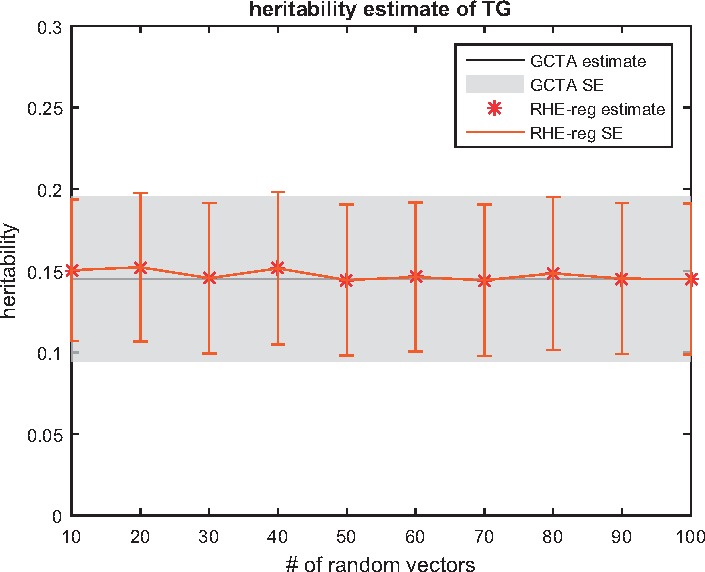
Impact of the number of random vectors on the accuracy of RHE-reg: we ran RHE-reg with a different number of random vectors B, and compared the point estimate and standard error to GCTA. The gray area indicates the standard error computed by GCTA. As RHE-reg use more random vectors, the estimate converges. In fact, even with 10 random vectors, the point estimation is accurate

3 Results

3.1 Simulations

We performed simulations to measure the performance of RHE-reg to other methods for heritability estimation in terms of accuracy, running time and memory usage. We compared RHE-reg to two methods for computing REML estimates: GCTA (Yang et al., 2011) (which implements an exact numerical optimization algorithm to compute the REML) as well as implementations of HE-regression.

3.2 Accuracy

In our first set of simulations, we compared the accuracy of RHE-reg to our implementation of exact HE-regression as well as GCTA, an implementation that computes the REML. We simulated genotypes assuming each SNP is drawn independently from a Binomial distribution with allele frequency that is sampled uniformly from the interval (0, 1). Given the genotypes, we simulated phenotypes under an infinitesimal model, i.e. with effect size at each SNP drawn independently from a normal distribution with mean zero and variance equal to the heritability divided by the number of SNPs. We considered different values for the true SNP heritability of the phenotype to be 0.2, 0.5 and 0.8.

In our first series of experiments, we fixed the number of SNPs at M = 10 000 and varied the number of individuals $N=1k,2k\dots 10k$. In the second series of experiments, we varied the number of SNPs $M=1k,2k\dots 10k$ while fixing the number of individuals to be N = 10 000. We repeated each experiment 100 times in order to assess the variance of each of the estimators. We estimated heritability using RHE-reg with B = 100 random vectors.

Figure 1 compares the estimates of each of the three methods (RHE-reg, HE-regression and GCTA) to the true heritability. First, we observe that all three methods obtain estimates of heritability that are quite close to each other as well as to the true heritability across the range of parameters explored. Second, RHE-reg and HE-regression are virtually indistinguishable in the variance of their estimates in each configuration. This suggests that the randomization makes a negligible contribution to the statistical accuracy of the MoM estimators. In some cases, RHE-reg even has a smaller variance than HE-regression. Third, as expected, REML obtains estimators that are closer to the true heritability compared to either of the MoM estimators for a high value of true heritability. For lower values of true heritability ($h^2=0.20,h^2=0.50$), the estimates from REML, HE-regression and RHE-reg are comparable. This result is also expected given that REML is asymptotically equivalent to MoM when the phenotypic correlation between individuals is small (Sham et al., 2000; Sham and Purcell, 2001). Finally, the sample size has a bigger effect than the number of SNPs on the accuracy of each of the methods, consistent with theory (Visscher et al., 2014).

3.3 Computational efficiency

In the second set of simulations, we compared the runtime and memory usage of different methods. We compared RHE-reg to two REML methods, GCTA (Yang et al., 2011) and BOLT-REML (Loh et al., 2015a) (a computationally efficient approximate method to compute the REML) as well as an exact MoM method MMHE (Ge et al., 2017). In this experiment, we simulated genotype data consisting of 100 000 SNPs over sample sizes of $N=10k,20k,30k,50k,100k$ and 500 k and then simulated phenotypes corresponding to the genotype data. For each dataset, we ran RHE-reg with B = 100 random vectors. We performed all comparisons on an Intel(R) Xeon(R) CPU 2.10 GHz server with 128 GB RAM. All computations were restricted to a single core, capped to a maximum runtime of 12 h and a maximum memory of 128 GB.

Figure 3 shows that both GCTA and MMHE do not scale to large sample sizes due to the requirement of computing and operating on a GRM that scales quadratically with N. GCTA could not complete its computation when running on $N=100K$ individuals while MMHE did not complete its computation on $N=50K$. BOLT-REML and RHE-reg scale linearly with sample size. However, RHE-reg is an order of magnitude faster than BOLT-REML. For example, on a dataset of a size of 500 K individuals, RHE-reg computed the heritability in about 30 min compared to 400 min for BOLT-REML. Figure 3 shows that RHE-reg is memory efficient as well.

Fig. 3.

RHE-reg is efficient: we measured the run time and memory usage of methods for heritability estimation as a function of the number of samples while fixing the number of SNPs to 100 000. We performed all comparisons on an Intel(R) Xeon(R) CPU 2.10 GHz server with 128 GB RAM. All computations were restricted to a single core, capped to a maximum runtime of 12 h and a maximum memory of 128 GB. In (a), GCTA could not finish computation on 100 K samples. For MMHE, the computation stopped at sample size of 50 k due to memory constraints. Although BOLT-REML scales linearly, RHE-reg is significantly faster. In (b), we observe RHE-reg and BOLT-REML have scalable memory requirements

3.4 Application to real data

We compared the statistical accuracy and runtime of BOLT-REML, GCTA and RHE-reg on the Northern Finland Birth Cohort (NFBC) dataset. The NFBC dataset contains 315 529 SNPs and 5326 individuals after applying standard filters (minor allele frequency >0.05 and Hardy–Weinberg equilibrium P-value <0.01) (Sabatti et al., 2009). We applied these methods to estimate the heritability of three phenotypes that were assayed in this dataset: triglycerides (TGs), high-density lipoprotein (HDL) and body mass index (BMI).

We compared the runtime, point estimates of the heritability as well as standard errors for each of the three methods. We computed RHE-reg with B = 100 random vectors. As shown in Table 1, the heritability estimates of RHE-reg are concordant with the other methods while being an order of magnitude faster to compute. We note that the NFBC dataset has a sample size $N\approx 5000$ so that we expect RHE-reg to be more accurate on larger datasets. The standard error estimates can also be computed in sub-linear time (see Appendix A4).

Table 1.

The estimates of heritability from RHE-reg are consistent with those from GCTA and BOLT-REML on the NFBC data while RHE-reg is substantially faster

Method
	GCTA		BOLT-REML		RHE-reg
	Runtime	$h_g^2$	Runtime	$h_g^2$	Runtime	$h_g^2$
	(min)	(SE)	(min)	(SE)	(min)	(SE)
TG	11.28	0.145	8.87	0.148	1.61	0.145
	–	(0.051)	–	(0.051)	–	(0.052)
HDL	10.81	0.325	9.72	0.326	1.30	0.349
	–	(0.051)	–	(0.051)	–	(0.052)
BMI	10.85	0.237	9.29	0.235	1.29	0.200
	–	(0.051)	–	(0.051)	–	(0.052)

Note: We estimate the heritability of phenotypes such as triglycerides (TGs), high-density lipoprotein (HDL) and body mass index (BMI) in the NFBC data set.

3.5 Understanding the computational efficiency of RHE-reg

Our implementation of RHE-reg relies on two ideas to obtain computational efficiency: (i) the use of a randomized estimator of the trace, and (ii) the Mailman algorithm for fast matrix-vector multiplication. To explore the contribution of each of these ideas, we compared the runtimes of a MoM estimator with no randomization (HE-reg), RHE-reg using standard matrix-vector multiplication and RHE-reg using the Mailman algorithm. Table 2 shows the runtimes of each of these variants on the NFBC data. We see that the biggest runtime gain arises from applying the randomized estimator (faster by a factor of 10–12 relative to HE-reg) while the application of the Mailman algorithm reduces the runtime further by a factor of 2 (Table 1).

Table 2.

The major gain in computational efficiency arises from the application of the randomized trace estimate

	Runtime	No Mailman	No randomized
			trace estimate
	(min)	(min)	(min)
TG	1.61	3.70	38.5
HDL	1.30	2.60	36.2
BMI	1.29	2.68	36.7

Note: We compare the run time for HE-reg as well as the run time for RHE-reg that does not rely on the Mailman algorithm.

3.6 Accuracy of RHE-reg as a function of the number of random vectors B

To explore the impact of the choice of the number of random vectors B on the accuracy of RHE-reg, we compared the heritability estimates of RHE-reg to those obtained from GCTA for the TG phenotype as a function of B. We find good concordance between the estimates from RHE-reg and GCTA even for values of B as low as 10 suggesting that RHE-reg could be even faster in practice with little loss in accuracy (see Fig. 2).

4 Discussion

We proposed a scalable estimator of heritability which is a randomized version of the Haseman–Elston regression (RHE-reg) estimator. The RHE-reg estimator is based on performing a small number of multiplications of the genotype matrix with random vectors with mean zero and identity covariance. Using the properties of the genotype matrix, we can compute this estimator using the Mailman algorithm in $\mathcal{O}\left(\frac{NMB}{\max (\hspace{0.17em}{\text{log}}_{3}N,\hspace{0.17em}{\text{log}}_{3}M)}\right)$ time on a dataset containing N individuals, M SNPs and with a small number of B random vectors. We show that this estimator achieves similar accuracy as REML-based methods on both simulated and real data. RHE-reg can be effectively applied to whole-genome genotype data of hundreds of thousands of individuals for rapid variance components estimation. Furthermore, RHE-reg is an unbiased estimator and thus can also be applied to ascertained case-control studies.

Appendix

A1. Method-of-Moments

The MoM principle obtains estimates of the model parameters such that the theoretical moments match the sample moments. In our model, the first theoretical moment, $\mathbb{E}[\mathit{y}]$, is $\mathbf{0}$ by definition while the corresponding sample moment is also zero since we standardized the phenotypes. The second sample moment is $\mathit{y}{\mathit{y}}^T$ and the second theoretical moment is $cov(\mathit{y})={\sigma }_g^2\mathit{K}+{\sigma }_e^2{\mathit{I}}_N$. Thus, the MoM estimator of $({\sigma }_g^2,\hspace{0.17em}{\sigma }_e^2)$ is obtained by searching for values of ${\sigma }_g^2,\hspace{0.17em}{\sigma }_e^2$ such that the sample and theoretical moments are close, i.e. by solving an ordinary least squares (OLS) problem:

$$(\widehat{{\sigma }_g^2},\widehat{{\sigma }_e^2})=argmi{n}_{{\sigma }_g^2,{\sigma }_e^2}\left|\right|\mathit{y}{\mathit{y}}^T-({\sigma }_g^2\mathit{K}+{\sigma }_e^2\mathit{I})|{|}_F^2.$$

Since the Frobenius norm of a matrix $\mathit{A},\hspace{0.17em}\left|\right|\mathit{A}|{|}_F=\sqrt{\text{tr}[\mathit{A}{\mathit{A}}^T]}$, the OLS problem can be re-written as:

$$(\widehat{{\sigma }_g^2},\widehat{{\sigma }_e^2})=argmi{n}_{{\sigma }_g^2,{\sigma }_e^2}\text{tr}[(\mathit{y}{\mathit{y}}^T-({\sigma }_g^2\mathit{K}+{\sigma }_e^2\mathit{I})){(\mathit{y}{\mathit{y}}^T-({\sigma }_g^2\mathit{K}+{\sigma }_e^2\mathit{I}))}^T]$$

which leads to Equation (6).

A2. Randomized estimator of trace of a matrix

For a N × N matrix, $\mathit{A}$, a randomized estimator of $\text{tr}[\mathit{A}]$ is $\widehat{\text{tr}\left[\mathit{A}\right]}\equiv \frac{1}{B}\sum _b{\mathit{z}}_{\mathit{b}}T\mathit{A}{\mathit{z}}_{\mathit{b}}$, where ${\mathit{z}}_{\mathit{b}}$ are i.i.d. random vectors with each entry drawn from a standard normal distribution. To see this:

$$\begin{array}{l}\mathbb{E}[{\mathit{z}}^T\mathit{Az}]=\mathbb{E}[tr({\mathit{z}}^T\mathit{Az})]\hspace{1em}{\mathit{z}}^T\mathit{Az} \mathtt{is a scalar}\\ =\mathbb{E}[\text{tr}[\mathit{z}{\mathit{z}}^T\mathit{A}]]\hspace{1em}\mathtt{cyclic property of the trace}\\ =\text{tr}[\mathbb{E}[\mathit{z}{\mathit{z}}^T\mathit{A}]]\hspace{1em}\mathtt{trace and expectation are linear}\\ =\text{tr}[\mathbb{E}[\mathit{z}{\mathit{z}}^T]\mathit{A}]\mathit{A}\hspace{0.17em}\hspace{0.17em}\mathtt{is fixed}\\ =\text{tr}[\mathit{A}] \mathtt{using the distributional assumptions on }\mathit{z}.\end{array}$$

A3. Bias of the RHE-reg estimator

Our estimator of $\text{tr}\left[{\mathit{K}}^2\right]$ is $L_B\equiv \widehat{tr\left[K^2\right]}=\frac{1}{B}\sum _B{\mathit{z}}_b^T\mathit{KK}{\mathit{z}}_b$. The RHE-reg estimators for $({\sigma }_g^2,{\sigma }_e^2)$ are given by: $\left[\begin{array}{c}\widetilde{{\sigma }_g^2}\\ \widetilde{{\sigma }_e^2}\end{array}\right]={\mathit{A}}^{-1}\left[\begin{array}{c}{\mathit{y}}^T\mathit{Ky}\\ {\mathit{y}}^T\mathit{y}\end{array}\right]$ where $\mathit{A}=\left[\begin{array}{cc}{L}_B& N\\ N& N\end{array}\right]$.

We first compute the expectation of this estimator:

$$\begin{array}{c}\mathbb{E}\left[\begin{array}{c}\widetilde{{\sigma }_g^2}\\ \widetilde{{\sigma }_e^2}\end{array}\right]=\mathbb{E}\left[{\mathit{A}}^{-1}\left[\begin{array}{c}{\mathit{y}}^T\mathit{Ky}\\ {\mathit{y}}^T\mathit{y}\end{array}\right]\right]\\ =\mathbb{E}\left[{\mathit{A}}^{-1}\right]\mathbb{E}\left[\begin{array}{c}{\mathit{y}}^T\mathit{Ky}\\ {\mathit{y}}^T\mathit{y}\end{array}\right]\hspace{1em}\mathtt{since random vectors }{\mathit{z}}_b\mathtt{ and }\mathit{y}\mathtt{ are independent}\end{array}.$$

We know that $\mathbb{E}[\mathit{y}{\mathit{y}}^T]=cov(\mathit{y})={\sigma }_g^2\mathit{K}+{\sigma }_e^2\mathit{I}$. We can compute $\mathbb{E}[{\mathit{y}}^T\mathit{Ky}]$:

$$\begin{array}{l}\mathbb{E}\left[{\mathit{y}}^T\mathit{Ky}\right]=\mathbb{E}\left[\text{tr}\left[{\mathit{y}}^T\mathit{Ky}\right]\right]\hspace{1em}{\mathit{y}}^T\mathit{Ky} \mathtt{is a scalar}\\ =\mathbb{E}\left[\text{tr}\left[\mathit{y}{\mathit{y}}^T\mathit{K}\right]\right]\hspace{1em}\mathtt{cyclic property of the trace}\\ =\text{tr}\left[\mathbb{E}\left[\mathit{y}{\mathit{y}}^T\mathit{K}\right]\right]\hspace{1em}\mathtt{expectation and trace are }\mathtt{linear}\\ =\text{tr}\left[\mathbb{E}\left[\mathit{y}{\mathit{y}}^T\right]\mathit{K}\right]\hspace{1em}\mathtt{as }\mathit{K}\mathtt{ is constant}\\ =\text{tr}\left[{\sigma }_g^2{\mathit{K}}^2+{\sigma }_e^2\mathit{K}\right]\\ ={\sigma }_g^2\text{tr}\left[{\mathit{K}}^2\right]+N{\sigma }_e^2\hspace{1em}\mathtt{using }\text{tr}\left[K\right]=N.\end{array}$$

And for $\mathbb{E}[{\mathit{y}}^T\mathit{y}]$, we have;

$$\mathbb{E}[{\mathit{y}}^T\mathit{y}]=\mathbb{E}[\text{tr}[{\mathit{y}}^T\mathit{y}]]\hspace{1em}{\mathit{y}}^T\mathit{y} \mathtt{is a scalar}$$

$$\begin{array}{l}=\mathbb{E}(\text{tr}[\mathit{y}{\mathit{y}}^T]]\hspace{1em}\mathtt{cyclic property of the trace}\\ =\text{tr}[\mathbb{E}[\mathit{y}{\mathit{y}}^T]]\hspace{1em}\mathtt{expectation and trace are linear}\\ =\text{tr}[\mathit{K}]{\sigma }_g^2+N{\sigma }_e^2\\ =N{\sigma }_g^2+N{\sigma }_e^2.\end{array}$$

Defining $b\equiv \mathbb{E}\left[\frac{1}{L_B-N}\right]$ and computing ${\mathit{A}}^{-1}=\left[\begin{array}{cc}\frac{1}{L_B-N}& \frac{-1}{L_B-N}\\ \frac{-1}{L_B-N}& \frac{L_B}{N(L_B-N)}\end{array}\right]$, we have

$$\begin{array}{l}\mathbb{E}\left[\begin{array}{c}\widetilde{{\sigma }_g^2}\\ \widetilde{{\sigma }_e^2}\end{array}\right]=\mathbb{E}\left[{\mathit{A}}^{-1}\right]\mathbb{E}\left[\left[\begin{array}{c}{\mathit{y}}^T\mathit{Ky}\\ {\mathit{y}}^T\mathit{y}\end{array}\right]\right]\\ =\left[\begin{array}{cc}b& -b\\ -b& \frac{1}{N}+b\end{array}\right]\left[\begin{array}{c}\text{tr}\left[{\mathit{K}}^2\right]+N{\sigma }_e^2\\ N{\sigma }_g^2+N{\sigma }_e^2\end{array}\right]\\ =\left[\begin{array}{c}b(\text{tr}\left[{\mathit{K}}^2\right]-N){\sigma }_g^2\\ b(N-\text{tr}\left[{\mathit{K}}^2]\right]{\sigma }_g^2+{\sigma }_g^2+{\sigma }_e^2\end{array}\right].\end{array}$$

We approximate $b=\mathbb{E}\left[\frac{1}{L_B-N}\right]$ using Taylor expansion. As we have: $f\left(y\right)\approx f\left(x\right)+f^{\prime }\left(x\right)(y-x)+\frac{1}{2}{f}^{″}\left(x\right){(y-x)}^2$. Let $X\equiv L_B-N$, and thus ${\mu }_x=\mathbb{E}[L_B-N]=\text{tr}\left[{\mathit{K}}^2\right]-N$. We have $f\left(x\right)=\frac{1}{x},f^{\prime }\left(x\right)=-\frac{1}{x^2},f^{″}\left(x\right)=\frac{2}{x^3}$.

Thus:

$$\begin{array}{c}b=\mathbb{E}\left[f\right(X\left)\right]\approx \mathbb{E}\left[f\right({\mu }_x)+f^{\prime }({\mu }_x\left)\right(X-{\mu }_x)+\frac{1}{2}{f}^{″}({\mu }_x\left){(X-{\mu }_x)}^2\right]\\ =f\left({\mu }_x\right)+\frac{1}{-{\mu }_x^2}\mathbb{E}[X-{\mu }_x]+\frac{1}{2}\frac{2}{{\mu }_x^3}\mathbb{E}[{(X-{\mu }_x)}^2\\ =\frac{1}{{\mu }_x}+\frac{1}{{\mu }_x}\frac{{\sigma }_x^2}{{\mu }_x^2}]\end{array}$$

where ${\sigma }_x^2=var\left(X\right)$.

Thus $\mathbb{E}\left[\frac{{\mu }_x}{x}\right]=1+\frac{{\sigma }_x^2}{{\mu }_x^2}$. Thus $\mathbb{E}\left[\widetilde{{\sigma }_g^2}\right]={\sigma }_g^2+\frac{{\sigma }_x^2}{{\mu }_x^2}{\sigma }_g^2,\hspace{0.17em}\mathbb{E}\left[{\sigma }_e^2\right]={\sigma }_e^2-\frac{{\sigma }_x^2}{{\mu }_x^2}{\sigma }_g^2,\hspace{0.17em}\mathbb{E}[\widetilde{{\sigma }_g^2}+\widetilde{{\sigma }_e^2}]={\sigma }_g^2+{\sigma }_e^2$.

For ${\sigma }_x^2$, we have:

$$\begin{array}{l}{\sigma }_x^2=\mathbb{E}\left[{(L_B-\text{tr}\left[{\mathit{K}}^2\right])}^2\right]\\ =var\left(L_B\right)\\ =var\left(\frac{1}{B}\sum _B{\mathit{z}}_b^T{\mathit{K}}^2{\mathit{z}}_b\right)\hspace{1em}{\mathit{z}}_b\hspace{0.17em}\mathtt{are independent}\\ =\frac{1}{B^2}\sum _{B}var\left({\mathit{z}}_b^T{\mathit{K}}^2{\mathit{z}}_b\right)\hspace{1em}{\mathit{z}}_b\hspace{0.17em}\mathtt{are identically distributed}\\ =\frac{1}{B}\sum _{i,j}{\mathit{K}}_i^T{\mathit{K}}_j{\mathit{z}}_i{\mathit{z}}_j\hspace{1em}\mathtt{elements of }\mathit{z}\mathtt{ are independent}\\ =\frac{1}{B}\sum _i{\mathit{K}}_i^2=\frac{1}{B}\text{tr}\left[{\mathit{K}}^2\right].\end{array}$$

Here ${\mathit{K}}_i$ is the ith column of K.

Thus, substituting μ_x and ${\sigma }_x^2$, we get $\mathbb{E}\left[\widetilde{{\sigma }_g^2}\right]={\sigma }_g^2+\frac{1}{B}\frac{\text{tr}\left[{\mathit{K}}^2\right]}{{(\text{tr}\left[{\mathit{K}}^2\right]-N)}^2}{\sigma }_g^2={\sigma }_g^2+\frac{1}{B}\frac{1}{\text{tr}\left[{\mathit{K}}^2\right]-2N+\frac{N^2}{\text{tr}\left[{\mathit{K}}^2\right]}}{\sigma }_g^2$. The bias of the estimator decreases with larger number of random vectors B.

A4. Standard error estimate for the RHE-reg estimator

We define $var\left(\mathit{y}\right)\equiv \Sigma ={\sigma }_g^2\mathit{K}+{\sigma }_e^2\mathit{I}$. As we know $\widetilde{{\sigma }_g^2}=\frac{{\mathit{y}}^T(\mathit{K}-\mathit{I})\mathit{y}}{L_B-N}$. Let $\widetilde{{\sigma }_g^2}\equiv \frac{A}{B}$ where $A\equiv y^T(K-I)y$ and $B\equiv L_B-N$. Define ${\mu }_A\equiv \mathbb{E}\left[A\right],\hspace{0.17em}{\mu }_B\equiv \mathbb{E}\left[B\right],\hspace{0.17em}{\sigma }_A^2\equiv var\left(A\right)$ and ${\sigma }_B^2\equiv var\left(B\right)$. From Lemma 2 (Appendix A5), we have

$$\begin{array}{l}var\left(\widetilde{{\sigma }_g^2}\right)=var\left(\frac{A}{B}\right)\\ =\frac{1}{{\left({\mu }_B\right)}^2}{\sigma }_A^2-2\frac{{\mu }_A}{{\left({\mu }_B\right)}^3}cov(A,B)+\frac{{\left({\mu }_A\right)}^2}{{\left({\mu }_B\right)}^4}{\sigma }_B^2\\ =\frac{1}{{\left({\mu }_B\right)}^2}{\sigma }_A^2+\frac{{\left({\mu }_A\right)}^2}{{\left({\mu }_B\right)}^4}{\sigma }_B^2\end{array}$$

as A, B are independent. By using Lemma 1 (Appendix A5), we have:

$$\begin{array}{l}{\mu }_A=\mathbb{E}\left[{\mathit{y}}^T\right(\mathit{K}-\mathit{I}\left)\mathit{y}\right]=(\text{tr}\left[{\mathit{K}}^2\right]-N){\sigma }_g^2\\ {\sigma }_A^2=var\left({\mathit{y}}^T\right(\mathit{K}-\mathit{I}\left)\mathit{y}\right)=2\text{tr}\left[\mathbf{\Sigma }(\mathit{K}-\mathit{I})\mathbf{\Sigma }(\mathit{K}-\mathit{I})\right]\\ {\mu }_B=\text{tr}\left[{\mathit{K}}^2\right]-N\\ {\sigma }_B^2=\frac{\text{tr}\left[{\mathit{K}}^2\right]}{B}.\end{array}$$

Thus we have:

$$SE\left(\widetilde{{\sigma }_g^2}\right)=\frac{1}{\text{tr}\left[{\mathit{K}}^2\right]-N}\sqrt{2\text{tr}\left[\mathbf{\Sigma }(\mathit{K}-\mathit{I})\mathbf{\Sigma }(\mathit{K}-\mathit{I})\right]+\frac{1}{B}{\left({\sigma }_g^2\right)}^2\text{tr}\left[{\mathit{K}}^2\right]}.$$

In order to estimate the standard error of $\widetilde{{\sigma }_g^2}$, we use the plug-in estimator:

$$\widehat{SE\left(\widetilde{{\sigma }_g^2}\right)}=\frac{1}{L_B-N}\sqrt{2\text{tr}\left[\mathit{y}{\mathit{y}}^T(\mathit{K}-\mathit{I})\mathbf{\Sigma }(\mathit{K}-\mathit{I})\right]+\frac{1}{B}{\left(\widetilde{{\sigma }_g^2}\right)}^2{L}_B}.$$ (15)

Each term in this estimator could be efficiently computed in $O\left(\frac{NMB}{\max (\hspace{0.17em}{\text{log}}_{3}N,\hspace{0.17em}{\text{log}}_{3}M)}\right).$

A5. Useful identities

Lemma 1. For a random vector $\mathit{z}$ that is distributed according to a multivariate normal distribution: $\mathit{z}\sim \mathcal{N}(0,\mathit{C})$ and for symmetric matrices $\mathit{A}$ and $\mathit{B}$.

$$cov({\mathit{z}}^T\mathit{Az},{\mathit{z}}^T\mathit{Bz})=2\text{tr}\left[\mathit{CACB}\right].$$

Thus

$$\begin{array}{c}\mathbb{E}\left[\right({\mathit{z}}^T\mathit{Az}\left)\right({\mathit{z}}^{T}B\mathit{z}\left)\right]=2\text{tr}\left[\mathit{CACB}\right]+\mathbb{E}\left[\right({\mathit{z}}^T\mathit{Az}\left)\right]\mathbb{E}\left[\right({\mathit{z}}^T\mathit{Bz}\left)\right]\\ =2\text{tr}\left[\mathit{CACB}\right]+\text{tr}\left[\mathit{AC}\right]\text{tr}\left[\mathit{BC}\right].\end{array}$$

Lemma 2. For two random variables, A and B, where B is either discrete or has support (0,$\infty$), and $\mathbb{E}\left[A\right]={\mu }_A,\hspace{0.17em}\mathbb{E}\left[B\right]={\mu }_B$.

$$var\left(\frac{A}{B}\right)\approx \frac{1}{{\left({\mu }_B\right)}^2}var\left(A\right)+2\frac{-{\mu }_A}{{\left({\mu }_B\right)}^3}cov(A,B)+\frac{{\left({\mu }_A\right)}^2}{{\left({\mu }_B\right)}^4}var\left(B\right).$$

References

- Almasy L., Blangero J. (1998) Multipoint quantitative-trait linkage analysis in general pedigrees. Am. J. Hum. Genet., 62, 1198–1211. [DOI] [PMC free article] [PubMed] [Google Scholar]
- Bulik-Sullivan B. (2015) Relationship between ld score and Haseman-Elston regression. bioRxiv, 018283.
- Chen G.-B. (2014) Estimating heritability of complex traits from genome-wide association studies using ibs-based Haseman–Elston regression. Front. Genet., 5, 107.. [DOI] [PMC free article] [PubMed] [Google Scholar]
- Chen W.-M. et al. (2004) Quantitative trait linkage analysis by generalized estimating equations: unification of variance components and Haseman-Elston regression. Genet. Epidemiol., 26, 265–272. [DOI] [PubMed] [Google Scholar]
- Elston R.C. et al. (2000) Haseman and Elston revisited. Genet. Epidemiol., 19, 1–17. [DOI] [PubMed] [Google Scholar]
- Ge T. et al. (2017) Phenome-wide heritability analysis of the UK Biobank. PLoS Genet., 13, e1006711.. [DOI] [PMC free article] [PubMed] [Google Scholar]
- Golan D. et al. (2014) Measuring missing heritability: inferring the contribution of common variants. Proc. Natl. Acad. Sci., 111, E5272–E5281. [DOI] [PMC free article] [PubMed] [Google Scholar]
- Haseman J., Elston R. (1972) The investigation of linkage between a quantitative trait and a marker locus. Behav. Genet., 2, 3–19. [DOI] [PubMed] [Google Scholar]
- Houle D. (1992) Comparing evolvability and variability of quantitative traits. Genetics, 130, 195–204. [DOI] [PMC free article] [PubMed] [Google Scholar]
- Kang H.M. et al. (2008a) Accurate discovery of expression quantitative trait loci under confounding from spurious and genuine regulatory hotspots. Genetics, 180, 1909–1925. [DOI] [PMC free article] [PubMed] [Google Scholar]
- Kang H.M. et al. (2008b) Efficient control of population structure in model organism association mapping. Genetics, 178, 1709–1723. [DOI] [PMC free article] [PubMed] [Google Scholar]
- Liberty E., Zucker S.W. (2009) The Mailman algorithm: a note on matrix–vector multiplication. Inf. Process. Lett., 109, 179–182. [Google Scholar]
- Lippert C. et al. (2011) FaST linear mixed models for genome-wide association studies. Nat. Methods, 8, 833–835. [DOI] [PubMed] [Google Scholar]
- Loh P.-R. et al. (2015a) Contrasting genetic architectures of schizophrenia and other complex diseases using fast variance-components analysis. Nat. Genet., 47, 1385. [DOI] [PMC free article] [PubMed] [Google Scholar]
- Loh P.-R. et al. (2015b) Efficient bayesian mixed-model analysis increases association power in large cohorts. Nat. Genet., 47, 284.. [DOI] [PMC free article] [PubMed] [Google Scholar]
- Makowsky R. et al. (2011) Beyond missing heritability: prediction of complex traits. PLoS Genet., 7, e1002051.. [DOI] [PMC free article] [PubMed] [Google Scholar]
- Pirinen M. et al. (2013) Efficient computation with a linear mixed model on large-scale data sets with applications to genetic studies. Annal. Appl. Stat., 7, 369–390. [Google Scholar]
- Sabatti C. et al. (2009) Genome-wide association analysis of metabolic traits in a birth cohort from a founder population. Nat. Genet., 41, 35–46. [DOI] [PMC free article] [PubMed] [Google Scholar]
- Sham P., Purcell S. (2001) Equivalence between Haseman-Elston and variance-components linkage analyses for sib pairs. Am. J. Hum. Genet., 68, 1527–1532. [DOI] [PMC free article] [PubMed] [Google Scholar]
- Sham P. et al. (2000) Power of linkage versus association analysis of quantitative traits, by use of variance-components models, for sibship data. Am. J. Hum. Genet., 66, 1616–1630. [DOI] [PMC free article] [PubMed] [Google Scholar]
- Speed D. et al. (2012) Improved heritability estimation from genome-wide snps. Am. J. Hum. Genet., 91, 1011–1021. [DOI] [PMC free article] [PubMed] [Google Scholar]
- Visscher P.M. et al. (2008) Heritability in the genomics era? Concepts and misconceptions. Nat. Rev. Genet., 9, 255.. [DOI] [PubMed] [Google Scholar]
- Visscher P.M. et al. (2014) Statistical power to detect genetic (co) variance of complex traits using snp data in unrelated samples. PLoS Genet., 10, e1004269.. [DOI] [PMC free article] [PubMed] [Google Scholar]
- Wray N.R. et al. (2013) Pitfalls of predicting complex traits from snps. Nat. Rev. Genet., 14, 507.. [DOI] [PMC free article] [PubMed] [Google Scholar]
- Yang J. et al. (2010) Common snps explain a large proportion of the heritability for human height. Nat. Genet., 42, 565.. [DOI] [PMC free article] [PubMed] [Google Scholar]
- Yang J. et al. (2011) GCTA: a tool for genome-wide complex trait analysis. Am. J. Hum. Genet., 88, 76–82. [DOI] [PMC free article] [PubMed] [Google Scholar]
- Yu J. et al. (2006) A unified mixed-model method for association mapping that accounts for multiple levels of relatedness. Nat. Genet., 38, 203.. [DOI] [PubMed] [Google Scholar]
- Zhou X., Stephens M. (2014) Efficient multivariate linear mixed model algorithms for genome-wide association studies. Nat. Methods, 11, 407.. [DOI] [PMC free article] [PubMed] [Google Scholar]
- Zhou X. et al. (2013) Polygenic modeling with bayesian sparse linear mixed models. PLoS Genet., 9, e1003264.. [DOI] [PMC free article] [PubMed] [Google Scholar]