Optimal Mass Transport: Signal processing and machine-learning applications

Abstract

Transport-based techniques for signal and data analysis have received increased attention recently. Given their ability to provide accurate generative models for signal intensities and other data distributions, they have been used in a variety of applications including content-based retrieval, cancer detection, image super-resolution, and statistical machine learning, to name a few, and shown to produce state of the art results in several applications. Moreover, the geometric characteristics of transport-related metrics have inspired new kinds of algorithms for interpreting the meaning of data distributions. Here we provide a practical overview of the mathematical underpinnings of mass transport-related methods, including numerical implementation, as well as a review, with demonstrations, of several applications. Software accompanying this tutorial is available at [43].

I. Introduction

A. Motivation and goals

Numerous applications in science and technology depend on effective modeling and information extraction from signal and image data. Examples include being able to distinguish between benign and malignant tumors from medical images, learning models (e.g. dictionaries) for solving inverse problems, identifying people from images of faces, voice profiles, or fingerprints, and many others. Techniques based on the mathematics of optimal mass transport, also known as Earth Mover’s distance in engineering-related fields, have received significant attention recently given their ability to incorporate spatial (in addition to intensity) information when comparing signals, images, and other data sources, thus giving rise to different geometric interpretations of data distributions. These techniques have been used to simplify and augment the accuracy of numerous pattern recognition-related problems. Some examples covered in this tutorial include image retrieval [32, 44], signal and image representation [25, 27, 40, 50], inverse problems [30], cancer detection [4, 39], texture and color modeling [18, 41], shape and image registration [22, 29], and machine learning [12, 17, 19, 28, 36, 42], to name a few. This tutorial is meant to serve as an introductory guide to those wishing to familiarize themselves with these emerging techniques. Specifically we

• provide a brief overview of key mathematical concepts related to optimal mass transport

• describe recent advances in transport related methodology and theory

• provide a practical overview of their applications in modern signal analysis, modeling, and learning problems.

Software accompanying this tutorial is available at [43].

B. Why transport?

In recent years numerous techniques for signal and image analysis have been developed to address important learning and estimation problems. Researchers working to find solutions to these problems have found it necessary to develop techniques to compare signal intensities across different signal/image coordinates. A common problem in medical imaging, for example, is the analysis of magnetic resonance images with the goal of learning brain morphology differences between healthy and diseased populations. Decades of research in this area have culminated with techniques such as voxel and deformation-based morphology which make use of nonlinear registration methods to understand differences in tissue density and locations. Likewise, the development of dynamic time warping techniques was necessary to enable the comparison of time series data more meaningfully, without confounds from commonly encountered variations in time. Finally, researchers desiring to create realistic models of facial appearance have long understood that appearance models for eyes, lips, nose, etc. are significantly different and must thus be dependent on position relative to a fixed anatomy. The pervasive success of these, as well as other techniques such as optical flow, level-set methods, deep neural networks, for example, have thus taught us that 1) nonlinearity and 2) modeling the location of pixel intensities are essential concepts to keep in mind when solving modern regression problems related to estimation and classification.

The methodology mentioned above for modeling appearance and learning morphology, time series analysis and predictive modeling, deep neural networks for classification of sensor data, etc., is algorithmic in nature. The transport-related techniques reviewed below are nonlinear methods that, unlike linear methods such as Fourier, wavelets, and dictionary models, for example, explicitly model jointly signal intensities as well as their locations. Furthermore, they are often based on the theory of optimal mass transport from which fundamental principles can be put to use. Thus they hold the promise to ultimately play a significant role in the development of a theoretical foundation for certain subclasses of modern learning and estimation problems.

C. Overview and outline

As detailed below in section II, the optimal mass transport problem first arose due to Monge [35]. It was later expanded by Kantorovich [23] and found applications in operations research and economics. Section III provides an overview of the mathematical principles and formulation of optimal transport-related metrics, their geometric interpretation, and related embedding methods and signal transforms. We also explain Brenier’s theorem [9], which helped pave the way for several practical numerical implementation algorithms, which are then explained in detail in section IV. Finally, in section V we review and demonstrate the application of transport-based techniques to numerous problems including: image retrieval, registration and morphing, color and texture analysis, image denoising and restoration, morphometry, super resolution, and machine learning. As mentioned above, software implementing the examples shown can be downloaded from [43].

II. A brief historical note

The optimal mass transport problem seeks the most efficient way of transforming one distribution of mass to another, relative to a given cost function. The problem was initially studied by the French mathematician Gaspard Monge in his seminal work “Mémoire sur la théorie des déblais et des remblais” [35] in 1781. In 1942, Leonid V. Kantorovich, who at that time was unaware of Monge’s work, proposed a general formulation of the problem by considering optimal mass transport plans, which as opposed to Monge’s formulation allows for mass splitting [23]. Kantorovich shared the 1975 Nobel Prize in Economic Sciences with Tjalling Koopmans for his work in the optimal allocation of scarce resources. Kantorovich’s contribution is considered as “the birth of the modern formulation of optimal transport” [49] and it made the optimal mass transport problem an active field of research in the following years.

A significant portion of the theory of the optimal mass transport problem was developed in the Nineties. Starting with Brenier’s seminal work on characterization, existence, and uniqueness of optimal transport maps [9], followed by Caffarelli’s work on regularity conditions of such mappings [10] and Gangbo and McCann’s work on geometric interpretation of the problem [20].

A more thorough history and background on the optimal mass transport problem can be found in Villani’s book “Optimal Transport: Old and New” [49] and Santambrogio’s book “Optimal transport for applied mathematicians” [45].

The significant contributions in mathematical foundations of the optimal transport problem together with recent advancements in numerical methods [6, 14, 31, 37] have spurred the recent development of numerous data analysis techniques for modern estimation and detection (e.g. classification) problems.

III. Formulation of the problem and methodology

In this section we first review both the continuous and ‘discrete’ formulations of the optimal transport problem (i.e. Monge’s and Kantorovich’s formulations). Next, we review the geometrical characteristics of the problem, and finally review the transport based signal/image embeddings. In the sections below we’ve elected to avoid measure-theoretic notation, and other detailed mathematical language, in lieu of a more informal and intuitive description of the problem. It is important to know, however, that certain mathematical precision is required to best understand the differences between Monge’s and Kantorivich’s formulation, their geometric interpretations, and so on. The interested reader may find useful to consult [24] for a more complete and mathematical description of the concepts explained below.

A. Optimal Transport: Formulation

Over the past century or so, the theory of optimal transport (earth mover’s distance) has developed two main formulations, one utilizing a continuous map (Monge’s formulation) and one utilizing what is called a transport plan (Kantarovich’s formulation) for assigning the spatial correspondence necessary for the related transport problem. While Monge’s continuous formulation is helpful in problems where a point-to-point assignment is desired, Kantarovich’s formulation is more general, and also covers the case of discrete (Dirac) masses (in our case signal intensities). These differ not only in mathematical formulation, but also has consequences with regards to their respective numerical solutions, as well as applications.

1) Monge’s continuous formulation

The Monge optimal mass transportation problem is formulated as follows. Consider two signals or images I₀ and I₁ defined over their respective domains Ω₀ and Ω₁. Here Ω₀ and Ω₁ are typically subsets of ℝ^d, and often can be taken as the unit square (or cube in 3D). While a detailed measure-theoretic formulation is typically required (see [24]) we bypass rigorous formulation here and simply assume that I₀(x) and I₁(y) correspond to signal intensities at positions x ∈ Ω₀ and y ∈ Ω₁. For digital signals, an interpolating model can be used to construct these functions defined over continuous domains from sampled discrete data. Except for extensions which are described below, the signals are required to be nonnegative. That is, I₀(x) ≥ 0 ∀x ∈ Ω₀ and I₁(y) ≥ 0 ∀y ∈ Ω₁. In addition, the total amount of signal (or mass) for both signals should be equal to the same constant (which is generally chosen to be 1): ${\displaystyle {\int }_{{\mathrm{\Omega }}_0}{I}_0\left(x\right)\mathit{dx}}={\displaystyle {\int }_{{\mathrm{\Omega }}_1}{I}_1\left(y\right)\mathit{dy}}=1$. In other words, I₀ and I₁ are assumed to be probability density functions (PDFs).

Monge’s optimal transportation problem is to find a function f : Ω₀ → Ω₁ that ‘pushes’ I₀ onto I₁ and minimizes the following objective function,

$$M\left(I_0,I_1\right)=\underset{f\in \mathit{MP}}{\inf }{\displaystyle {\int }_{{\mathrm{\Omega }}_0}c\left(x,f\left(x\right)\right)I_0\left(x\right)\mathit{dx}}$$ (1)

where c : Ω₀ × Ω₁ → ℝ⁺ is the cost of moving pixel intensity I₀(x) from x to f (x) (Monge considered the Euclidean distance as the cost function in his original formulation, c(x, f (x)) = |x − f (x)|), and MP stands for a measure preserving map that moves all the signal intensity from I₀ to I₁. That is, for a subset B ⊂ Ω₁ the MP requirement is that

$${\displaystyle {\int }_{\left\{x:f\left(x\right)\in B\right\}}{I}_0\left(x\right)\mathit{dx}}={\displaystyle {\int }_B{I}_1\left(y\right)\mathit{dy}}.$$ (2)

If f is one-to-one this just means that for A ⊂ Ω₀

$${\displaystyle {\int }_A{I}_0\left(x\right)\mathit{dx}}={\displaystyle {\int }_{f\left(A\right)}{I}_1\left(y\right)\mathit{dy}}.$$

Such maps f ∈ MP are sometimes called ‘transport maps’ or ‘mass preserving maps’. Simply put, the Monge formulation of the problem seeks to rearrange signal I₀ into signal I₁ while minimizing a specific cost function. In cases when f is smooth and one to one, then the requirement (2) can be written in a differential form as

$$\det \left(Df\left(x\right)\right)I_1\left(f\left(x\right)\right)=I_0\left(x\right)$$ (3)

almost everywhere, where D f is the Jacobian of f (see Figure 1, top panel). Note that both the objective function and the constraint in Equation (1) are nonlinear with respect to f (x). Hence, for over a century the answers to questions regarding existence and characterization of the Monge’s problem remained unknown.

Fig. 1.

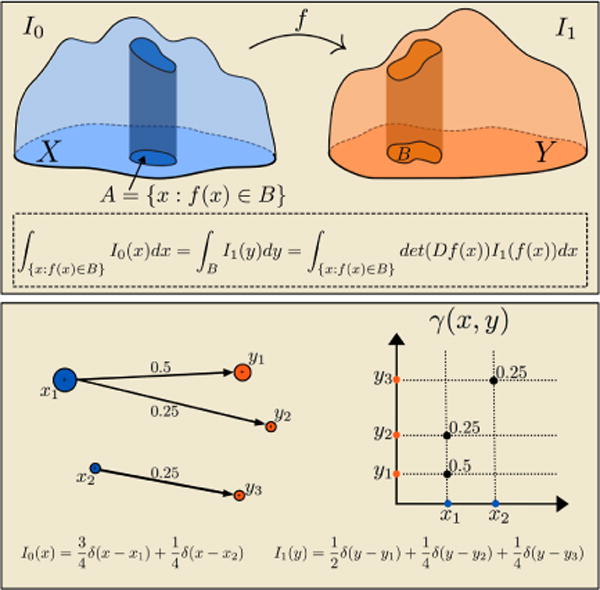
Monge transport map (top panel) and Kantorovich’s transport plan (bottom panel).

It should be mentioned that, for certain measures the Monge’s formulation of the optimal transport problem is ill-posed; in the sense that there is no transport map to rearrange one PDF to another. For instance, consider the case where I₀ is a Dirac mass while I₁ is not. Kantorovich’s formulation alleviates this problem by finding the optimal transport plan as opposed to the transport map.

2) Kantorovich’s formulation

Kantorovich formulated the transportation problem by optimizing over transportation plans, which we denote as γ. One can think of γ as the joint distribution of I₀ and I₁ describing how much ‘mass’ is being moved to different coordinates. That is let A be a subset of Ω₀ and similarly B ⊆ Ω₁. For notational simplicity we will not make a distinction between a probability distribution and its density. More precisely to a signal I₀ we associate a probability distribution by I₀(A) =∫_A I₀(x)dx.

The quantity γ(A × B) tells us how much ‘mass’ in set A is being moved to set B. Here the MP constraint can be expressed as γ(Ω₀×B) = I₁(B), and γ(A×Ω₁) = I₀(A). Kantorovich’s formulation for the optimal transport problem can then be written as,

$$K\left(I_0,I_1\right)=\underset{\gamma \in \mathit{MP}}{min}{\displaystyle {\int }_{{\mathrm{\Omega }}_0\times {\mathrm{\Omega }}_1}c\left(x,y\right)d\gamma \left(x,y\right)}.$$ (4)

Note that the measure theoretic notation above (the integration over dγ(x, y) above) is meant to represent the fact that this integral is more general than the routine Riemman-type integral commonly used in signal processing, and can cover ‘integration’ over domains which are more general. The minimizer of the optimization problem above, γ^∗, is called the optimal transport plan. Note that unlike the Monge problem, in Kantorovich’s formulation the objective function and the constraints are linear with respect to γ(x, y). Moreover, Kantorovich’s formulation is in the form of a convex optimization problem. We also note that the Monge problem is more restrictive than the Kantorovich problem. That is, in Monge’s version, mass from a single location in Ω₀ is being sent to a single location in Ω₁. Kantorovich’s formulation, however, considers transport plans which can deal with arbitrary measurable sets and has the ability to distribute mass from the one location in one density to multiple locations in another (see Figure 1, bottom panel). For any transport map f : Ω₀ → Ω₁ there is an associated transport plan, determined by

$$\gamma \left(A\times B\right)={\displaystyle {\int }_{\left\{x\in A:f\left(x\right)\in B\right\}}{I}_0\left(x\right)\mathit{dx}}.$$ (5)

Furthermore when an optimal transport map f^∗ exists, it can be shown that the transport plan γ^∗ derived from Equation 5 is an optimal transportation plan [49].

The Kantorovich problem is especially interesting in a discrete setting, that is for PDFs of the form $I_0={\displaystyle {\sum }_{i=1}^M{p}_i\delta \left(x-x_i\right)}$ and $I_1={\displaystyle {\sum }_{j=1}^N{q}_j\delta (y-y_j)}$, where δ(x) is the Dirac delta function. We note that for such PDFs in general there does not exist a transport map that ‘pushes’ I₀ into I₁. Namely the splitting of masses, which Kantorovich formulation allows, is necessary (see bottom panel of Figure 1). The Kantorovich problem can be written as,

$$K\left(I_0,I_1\right)=\underset{\gamma }{min}{\displaystyle \sum _i{\displaystyle \sum _{j}c(x_i,y_j){\gamma }_{\mathit{ij}}}}s.t.{\displaystyle \sum _j{\gamma }_{\mathit{ij}}=p_i},{\displaystyle \sum _i{\gamma }_{\mathit{ij}}=q_j}{\gamma }_{\mathit{ij}}\ge 0,i=1,\dots ,M,j=1,\dots ,N$$ (6)

where γ_ij identifies how much of the mass particle m_i at x_i needs to be moved to y_j (see Figure 1, bottom panel). Note that the optimization above has a linear objective function and linear constraints, therefore it is a linear programming problem. This problem is convex (which in practice translates to a relatively easier process of finding a global minimum), but not strictly so, and the constraint provides a polyhedral set of M × N matrices.

In practice, a non-discrete measure is often approximated by a discrete measure and the Kantorovich problem is solved through the linear programming optimization expressed in Equation (6).

3) Basic properties

Consider a transportation cost c(x, y) which is continuous and bounded from below. Given two signals I₀ and I₁ as above there always exists a transportation plan minimizing (4). This holds for both when signals I₀ and I₁ are functions and when they are discrete probability distributions [49].

A further important question is regarding the existence of an optimal transport map instead of a plan. Brenier [9] addressed this problem for the special case where c(x, y) = |x − y|². Bernier’s results was later relaxed to more general cases by Gangbo and McCann [20], which led to the following theorem:

Theorem

Let I₀ and I₁ be nonnegative functions of same total mass and with bounded support. When c(x, y) = h(x − y) for some strictly convex function h then there exists a unique optimal transportation map f^∗ minimizing (1). In addition, the optimal transport plan is unique, and given by (5). Moreover if c(x, y) = |x − y|² then there exists a (unique up to adding a constant) convex function ϕ such that f^∗ = ∇ϕ. A proof is available in [20, 49].

B. Optimal Mass Transport: Geometric properties

1) Wasserstein metric

Let Ω be a bounded subset of ℝ^d on which the signals are defined. For signals (d = 1) or images (d = 2), this can simply be the space [0, 1]^d, for example. Let P(Ω) be the set of probability densities supported on Ω. The p-Wasserstein metric, W_p, for p ≥ 1 on P(Ω) is then defined as using the optimal transportation problem (4) with the cost function c(x, y) = |x − y|^p. For I₀ and I₁ in P(Ω),

$$W_p\left(I_0,I_1\right)={\left(\underset{\gamma \in MP}{\inf }{\displaystyle {\int }_{\mathrm{\Omega }\times \mathrm{\Omega }}{\left|x-y\right|}^{p}d\gamma \left(x,y\right)}\right)}^{\frac{1}{p}}.$$

For any p ≥ 1, W_p is a metric on P(Ω). The metric space (P(Ω), W_p) is referred to as the p-Wasserstein space. To understand the nature of the optimal transportation distances it is useful to note that for any p ≥ 1, the convergence with respect to W_p is equivalent to the weak convergence of measures. That is W_p(I_n, I) → 0 as n → ∞ if and only if for every bounded and continuous function f : Ω → ℝ

$${\displaystyle {\int }_{\mathrm{\Omega }}f\left(x\right)I_n\left(x\right)\mathit{dx}\to }{\displaystyle {\int }_{\mathrm{\Omega }}f\left(x\right)I\left(x\right)\mathit{dx}.}$$

For the specific case of p = 1 the p-Wasserstein metric is also known as the Monge–Rubinstein [49] metric, or the earth mover distance [44]. The p-Wasserstein metric in one-dimension has a simple characterization. For one-dimensional signals I₀ and I₁ the optimal transport map has a closed form solution. Let F_i be the cumulative distribution function of I_i for i = 0, 1. That is

$$F_i\left(x\right)={\displaystyle {\int }_{\inf \left(\mathrm{\Omega }\right)}^x{I}_i\left(x\right)\mathit{dx}}\mathrm{for}i=0,1.$$

Note that this is a nondecreasing function going from 0 to 1. We define the pseudoinverse of F₀ as follows: for z ∈ (0, 1), F⁻¹(z) is the smallest x for which F₀(x) ≥ z, that is

$$F_0^{-1}\left(z\right)=\inf \left\{x\in \mathrm{\Omega }:F_0\left(x\right)\ge z\right\}$$

If I₀ > 0 then F₀ is continuous and increasing (and thus invertible) and the inverse of the function F₀ is equal to the pseudoinverse we just defined. In other words the pseudoinverse is a generalization of the notion of the inverse of a function. The pseudoinverse (i.e. the inverse if I₀ > 0 and I₁ > 0) provides a closed form solution for the p-Wasserstein distance:

$$W_p\left(I_0,I_1\right)={\left({\displaystyle {\int }_0^1{|F_0^{-1}\left(z\right)-F_1^{-1}\left(z\right)|}^p\mathit{dz}}\right)}^{\frac{1}{p}}.$$ (7)

The closed-form solution of the p-Wasserstein distance in one dimension is an attractive property, as it alleviates the need for optimization. This property was employed in the Sliced Wasserstein metrics as defined below.

2) Sliced-Wasserstein Metric

The idea behind the Sliced Wasserstein metric is to first obtain a set of one-dimensional representations for a higher-dimensional probability distribution through projections (slicing the measure), and then calculate the distance between two input distributions as a functional on the Wasserstein distance of their one-dimensional representations. In this sense, the distance is obtained by solving several one-dimensional optimal transport problems, which have closed-form solutions.

Projection of high-dimensional PDFs is closely related to the well known Radon transform in the imaging and image processing community [8, 25]. The d-dimensional Radon transform ℛ maps a function I ∈ L₁ (ℝ^d) where $L_1({ℝ}^d):=\{I:{ℝ}^d\to ℝ|{\displaystyle {\int }_{{ℝ}^d}|I(x)|dx\le \infty }\}$ into the of its integrals over the hyperplanes of ℝ^d and is defined as,

$$ℛI\left(t,\theta \right):={\displaystyle {\int }_{ℝ}I(t\theta +s{\theta }^{\perp })\mathit{ds}},\forall t\in ℝ,\forall \theta \in {\mathbb{S}}^{d-1}$$

here θ^⊥ is the subspace orthogonal to θ, and ${\mathbb{S}}^{d-1}$ is the unit sphere in ℝ^d. Note that $L_1({ℝ}^d)\to L_1(ℝ\times {\mathbb{S}}^{d-1})$. In other words, Radon transform projects a PDF, I ∈ P(ℝ^d), where d > 1, into an infinite set of one-dimensional PDFs ℛI(., θ). The Sliced Wasserstein metric for PDFs I₀ and I₁ on ℝ^d is then defined as,

$$S{W}_p\left(I_0,I_1\right)={\left({\displaystyle {\int }_{{\mathbb{S}}^{d-1}}{W}_p^p\left(ℛI_0\left(.,\theta \right),ℛI_1\left(.,\theta \right)\right)d\theta }\right)}^{\frac{1}{p}}$$

where p ≥ 1, and W_p is the p-Wasserstein metric, which for one dimensional PDFs ℛI₀(., θ) and ℛI₁(., θ) has a closed form solution (see Equation (7)). For more details and definitions of the Sliced Wasserstein metric we refer the reader to [8, 25, 29].

3) Wasserstein spaces, geodesics, and Riemannian structure

In this section we assume that Ω is convex. Here we highlight that the p-Wasserstein space (P(Ω), W_p) is not just a metric space, but has additional geometric structure. In particular for any p ≥ 1 and any I₀, I₁ ∈ P(Ω) there exists a continuous path (interpolation) between I₀ and I₁ whose length is the distance between I₀ and I₁.

Furthermore the space with p = 2 is special as it possesses a structure of a formal, infinite dimensional, Riemannian manifold. That structure was first noted by Otto [38] who developed the formal calculations for using this structure. Let us mention that the precise description of the manifold of probability measures endowed with Wasserstein metric can be found in Ambrosio, Gigli and Savaré [1].

Here we review the two main notions, which have a wide use. Namely we characterize the geodesics in (P(Ω), W_p) and in the case p = 2 describe what is the local, Riemannian metric of (P(Ω), W₂). Finally we state the seminal result of Benamou and Brenier [5] who provided a characterization of geodesics via action minimization which is useful in computations and also gives an intuitive explanation of the Wasserstein metric.

We first recall the definition of the length of a curve in a metric space. Let (X, d) be a metric space and I : [a, b] → X. Then the length of I, denoted by L(I) is

$$L\left(I\right)=\underset{m\in \mathbb{N},a=t_0<t_1<\cdots <t_m=b}{\sup }{\displaystyle \sum _{i=1}^{m}d\left(I\left(t_{i-1}\right),I\left(t_i\right)\right)}.$$

A metric space (X, d) is a geodesic space if for any I₀ and I₁ there exists a curve I : [0, 1] → X such that I(0) = I₀, I(1) = I₁ and for all 0 ≤ s < t ≤ 1, d(I(s), I(t)) = L(I|_[s,t]). In particular the length of I is equal to the distance from I₀ to I₁. Such a curve I is called a geodesic. The existence of geodesics is useful as it allows one to define the average of I₀ and I₁ as the midpoint of the geodesic connection them.

An important property of (P(Ω), W_p) is that it is a geodesic space and that geodesics are easy to characterize. Namely they are given by the displacement interpolation (a.k.a. McCann interpolation). When there exists a unique transportation map f* from I₀ to I₁ which min minimizes (1) for c(x; y) = |x − y|^p, the geodesic is obtained by moving the mass at constant speed from x to f*(x). More precisely, for t ∈ [0; 1] and x ∈ Ω let

$$f_t^{\ast }\left(x\right)=\left(1-t\right)x+t{f}^{\ast }\left(x\right)$$

be the position at time t of the mass initially at x. Note that $f_0^{\ast }$ is identity mapping and $f_1^{\ast }=f^{\ast }$. Pushing forward the mass by $f_t^{\ast }$ which by (3) has the form

$$I_t(f_t^{\ast }(x))=\frac{I_0(x)}{\det (D{f}_t^{\ast }(x))}$$

if f^∗ is smooth, provides the desired geodesic from I₀ to I₁. We remark that the velocity of each particle ${\partial }_t{f}_t^{\ast }=f^{\ast }\left(x\right)-x$ is the displacement of the optimal transportation map. Figure 2 conceptualizes the geodesic between two PDFs in P(Ω), and visualizes it for three different pairs of PDFs.

Fig. 2.

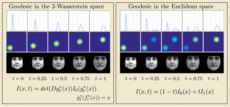
Geodesics in the 2-Wasserstein space (left panel), and in the Euclidean space (right panel) between various one and two-dimensional PDFs. Note that the geodesic in the 2-Wasserstein space captures the nonlinear structure of the signals and images and provides a natural morphing.

An important fact regarding the 2-Wasserstein space is Otto’s presentation of a formal Riemannian metric for this space [38]. It involves shifting to Lagrangian point of view. To explain, consider the path I(x, t) in P(Ω) with I(x, t) smooth. Then $s\left(x,t\right)=\frac{\partial I}{\partial t}\left(x,t\right)$ can be thought as a tangent vector to the manifold, or a density perturbation. Instead of thinking of increasing/decreasing the density this perturbation can be viewed as resulting from moving the mass by a vector field. In other words consider vector fields v(x, t) such that

$$s=-\nabla \cdot \left(Iv\right).$$ (8)

There are many such vector fields. Otto defined the size of s(·, t) as the square root of the minimal kinetic energy of the vector field that produces the perturbation to density s. That is

$$\langle s,s\rangle =\underset{v\mathrm{satisfied}\left(8\right)}{min}{\displaystyle \int {\left|v\right|}^{2}I\mathit{dx}}$$ (9)

Utilizing the Riemmanian manifold structure of P(Ω) together with the inner product presented in Equation (9) the 2-Wasserstein metric can be reformulated into finding the minimizer of the following action among all curves in P(Ω) connecting I₀ and I₁ [5],

$$W_2^2\left(I_0,I_1\right)={\inf }_{I,v}{\displaystyle {\int }_0^1{\displaystyle {\int }_{\mathrm{\Omega }}I\left(x,t\right){\left|v\left(x,t\right)\right|}^2\mathit{dxdt}}}$$

such that ∂_tI + ∇ · (Iv) = 0

$$I\left(\cdot ,0\right)=I_0(\cdot ),I\left(\cdot ,1\right)=I_1(\cdot )$$

where the first constraint is the well-known continuity equation.

C. Optimal Transport: Embeddings and Transforms

The optimal transport problem and specifically the 2-Wasserstein metric and the Sliced 2-Wasserstein metric have been recently used to define nonlinear transforms for signals and images [25, 27, 40, 50]. In contrast to commonly used linear signal transformation frameworks (e.g. Fourier and Wavelet transforms) which only employ signal intensities at fixed coordinate points, thus adopting an ‘Eulerian’ point of view, the idea behind the transport-based transforms is to consider the intensity variations together with the locations of the intensity variations in the signal. Therefore, such transforms adopt a ‘Lagrangian’ point of view for analyzing signals. That is, they are able to ‘move’ signal (pixel) intensities around. Moreover, the transforms can be viewed as Euclidean embeddings for the data, under the transport-related metric space structure described above. The benefit of such an Euclidean embedding is that they facilitate the application of many standard data analysis algorithms (e.g. learning). Here we briefly describe these transforms and some of their prominent properties.

1) The linear optimal transportation framework

The linear optimal transportation (LOT) framework was proposed by Wang et al. [50]. The framework was used in [4, 39] for pattern recognition in biomedical images and specifically histopathology and cytology images. Later, it was extended in [27] as a generic framework for pattern recognition and was used in [26] for single-frame super-resolution reconstruction of face images. The LOT framework provides an invertible Lagrangian transform for images. It was initially proposed as a method to simultaneously amend the computationally expensive requirement of calculating pairwise 2-Wasserstein distance between N signals for pattern recognition purposes, and to allow for the construction of generative models for images involving textures and shapes. For a given set of images I_i ∈ P₂(Ω), for i = 1, …, N, and a fixed template I₀, all non-negative and normalized to have the same sum, the transform projects the images to the tangent space at I₀. The projections are acquired by finding the optimal velocity fields corresponding to the optimal transport plans between I₀ and each image in the set.

The framework provides a linear embedding for P₂(Ω) with respect to a fixed signal I₀ ∈ P₂(Ω). Meaning that the Euclidean distance between an embedded signal, denoted as ${\stackrel{\sim }{I}}_i$, and the fixed reference, I₀, is equal to W₂(I₀, I_i) and the Euclidean distance between two embedded normalized signals is, generally speaking, an approximation of their 2-Wasserstein distance. The geometric interpretation of the LOT framework is presented in Figure 3. The linear embedding then facilitates the application of linear techniques such as principal component analysis (PCA) and linear discriminant analysis (LDA) to probability measures.

Fig. 3.

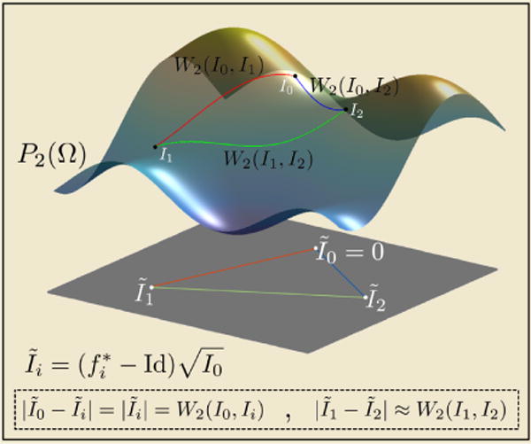
Graphical representation of the LOT framework. The framework embeds the PDFs (i.e. signals or images) I_i in the tangent space (i.e. the set of all tangent vectors) of P(Ω) with respect to a fixed PDF I₀. As a consequence, the Euclidean distance between the embedded functions ${\stackrel{\sim }{I}}_1$ and ${\stackrel{\sim }{I}}_2$ provides an approximation for the 2-Wasserstein distance, W₂(I₁, I₂).

2) The cumulative distribution transform

Park et al. [40] considered the LOT framework for one-dimensional PDFs (positive signals normalized to integrate to 1), and since in dimension one the transport maps are explicit, they were able to characterize the properties of the transformed densities. Here we briefly review their results. Similar to the LOT framework, let I_i for i = 1, …, N, and I₀ be signals (PDFs) defined on ℝ. The framework first calculates the optimal transport maps between I_i and I₀ using $f_i\left(x\right)=F_i^{-1}\circ F_0\left(x\right)$ for all i = 1, …, N. Then the forward and inverse transport-based transform, denoted as the cumulative distribution transform (CDT) by Park et al. [40], for these density functions with respect to the fixed template I₀ is defined as,

$$\{\begin{array}{cc}{\stackrel{\sim }{I}}_i=\left(f_i-\mathrm{Id}\right)\sqrt{I_0}& \left(\mathrm{Analysis}\right)\\ I_i={\left(f_i^{-1}\right)}^{\prime }\left(I_0\circ f_i^{-1}\right)& \left(\mathrm{Synthesis}\right)\end{array}$$

where $(I_0\circ f_i^{-1})(x)=I_0(f_i^{-1}(x))$. Note that the L₂-norm (Euclidean distance) of the transformed signals, ${\stackrel{\sim }{I}}_i$ corresponds to the 2-Wasserstein distance between I₀ and I_i. In contrast to the higher-dimensional LOT, the Euclidean distance between two transformed (embedded) signals ${\stackrel{\sim }{I}}_i$ and ${\stackrel{\sim }{I}}_j$, however, is the exact 2-Wasserstein distance between I_i and I_j (see [40] for a proof) and not just an approximation. Hence, the transformation is isometric (preserves) with respect to the 2-Wasserstein metric. This isometric nature of the CDT was utilized in [28] to provide positive definite kernels for machine learning of n-dimensional signals.

From a signal processing point of view, the CDT is a nonlinear signal transformation that captures certain nonlinear variations in signals including translation and scaling. Specifically, it gives rise to the transformation pairs presented in Table I. From Table I one can observe that although I(t − τ) is nonlinear in τ (when I(.) is not a linear function), its CDT representation $\stackrel{\sim }{I}\left(t\right)+\tau \sqrt{I_0\left(t\right)}$ becomes affine in τ (similar effect is observed for scaling). In effect, the Lagrangian transformations (compositions) in original signal space are rendered into Eulerian perturbations in transform space, borrowing from the PDE parlance. Furthermore, Park et al. [40] demonstrated that the CDT facilitates certain pattern recognition problems. More precisely, the transformation turns certain not linearly separable and disjoint classes of signals into linearly separable ones. Formally, let C be a set of 1D maps and let P, Q ⊂ P₂(Ω) be sets of positive PDFs born from two positive PDFs p₀, q₀ ∈ P₂(Ω) (which we denote as mother density functions or signals) as follows,

$$P=\{p|p=h^{\prime }(p_0\circ h),\forall h\in C\},Q=\{q|q=h^{\prime }(q_0\circ h),\forall h\in C\}.$$

If there exists no h ∈ C for which p₀ = h′(q₀ ◦ h) then the sets P and Q are disjoint but not necessarily linearly separable in the signal space. A main result of [40] states that the signal classes P and Q are guaranteed to be linearly separable in the transform space (regardless of the choice of the reference signal I₀) if C satisfies the following conditions,

1. h ∈ C ⇔ h⁻¹ ∈ C

2. h₁, h₂ ∈ C ⇒ ρh₁ + (1 − ρ)h₂ ∈ C, ∀ρ ∈ [0, 1]

3. h₁, h₂ ∈ C ⇒ h₁(h₂), h₂(h₁) ∈ C

4. h′(p₀ ◦ h) ≠ q₀, ∀h ∈ C

TABLE I.

Cumulative Distribution Transform pairs. Note that the composition holds for all strictly monotonically increasing functions g.

Cumulative Distribution Transform pairs
Property	Signal domain	CDT domain
	I (x)	$\stackrel{\sim }{I}(x)$
Translation	I (x − τ)	$\stackrel{\sim }{I}(x)+\tau \sqrt{I_0(x)}$
Scaling	aI (ax)	$\frac{\stackrel{\sim }{I}(x)}{a}-x\frac{(a-1)}{a}\sqrt{I_0(x)}$
Composition	g′ (x)I (g(x))	$(g^{-1}(\frac{\stackrel{\sim }{I}(x)}{\sqrt{I_0(x)}}+x)-x)\sqrt{I_0(x)}$

The set of translations C = {f | f (x) = x +τ, τ ∈ ℝ}, and scaling C = {f | f (x) = ax, a ∈ ℝ⁺}, for instance, satisfy the above conditions. We refer the reader to [40] for further reading. The top panel in Figure 4 demonstrates the linear separation property of the CDT. The signal classes P and Q are chosen to be the set of all translations of a single Gaussian and a Gaussian mixture including two Gaussian functions with a fixed mean difference, respectively. The discriminant subspace is calculated for these classes and it is shown that while the signal classes are not linearly separable in the signal domain, they become linearly separable in the transform domain.

Fig. 4.

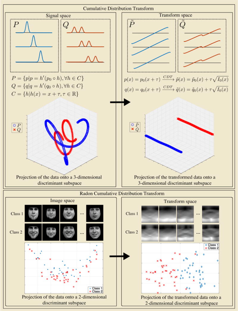
Examples for the linear separability characteristic of the CDT and the Radon-CDT. The discriminant subspace for each case is calculated using the penalized-linear discriminant analysis (p-LDA). It can be seen that the nonlinear structure of the data is well captured in the transform spaces.

3) The Radon cumulative distribution transform

The CDT framework was extended to 2 dimensional density functions (images) through the sliced-Wasserstein distance in [25], and was denoted as the Radon-CDT. It is shown in [25] that similar characteristics of the CDT, including the linear separation property, also hold for the Radon-CDT. Figure 4 clarifies the linear separation property of the Radon-CDT and demonstrate the capability of such transformations. Particularly, Figure 4 shows a facial expression dataset with two classes (i.e. neutral and smiling expressions) and its corresponding representations in the LDA discriminant subspace calculated from the images (bottom left panel), the Radon-CDT of the dataset and the corresponding representation of the transformed data in the LDA discriminant subspace (bottom right panel). It is clear that the image classes become more linearly separable in the transform space. In addition, the cumulative percentage variation of the dataset in the image space, the Radon transform space, the Ridgelet transform space, and the Radon-CDT space are shown in Figure 5. It can be seen that the variations in the dataset could be explained with fewer components in the Radon-CDT space.

Fig. 5.

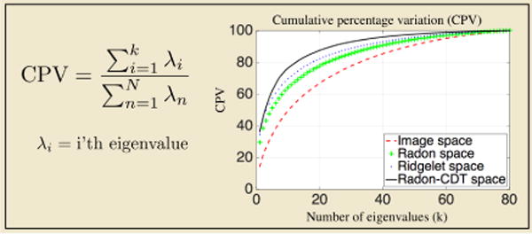
The cumulative percentage of the face dataset in Figure 4 in the image space, the Radon transform space, the Ridgelet transform space, and the Radon-CDT transform space.

IV. Numerical methods

The development of robust and efficient numerical methods for computing transport-related maps, plans, metrics, and geodesics, is crucial for the development of algorithms that can be used in practical applications. Below we present several notable approaches for finding transportation maps and plans. Table II provides a high-level overview of these methods.

TABLE II.

The key properties of various numerical approaches.

Comparison of Numerical Approaches
Method	Remark
linear programming	Applicable to general costs. Good approach if the PDFs are supported at very few sites
multi-scale linear programming	Applicable to general costs. Fast and robust method, though truncation involved can lead to imprecise distances.
Auction algorithm	Applicable only when the number of particles in the source and the target is equal and all of their masses are the same.
Entropy regularized linear programing	Applicable to general costs. Simple and performs very well in practice for moderately large problems. Difficult to obtain high accuracy.
Fluid mechanics	This approach can be adapted to generalizations of the quadratic cost, based on action along paths.
AHT minimization	Quadratic cost. Requires some smoothness and positivity of densities. Convergence is only guaranteed for infinitesimal stepsize.
Gradient descent on the dual problem	Quadratic cost. Convergence depends on the smoothness of the densities, hence a multi-scale approach is needed for non-smooth densities (i.e. normalized images).
Monge–Ampere solver	Quadratic cost. One in [7] is proved to be convergent. Accuracy is an issue due to wide stencil used.
Semi-discrete approximation	Efficient way to find map between a continuous and discrete signal [31].

A. Linear programming

The linear programming problem, is an optimization problem with a linear objective function and linear equality and inequality constraints. Several numerical methods exist for solving linear programming problems, among which are the simplex method and its variations and the interior-point methods. The computational complexity of the mentioned numerical methods, however, scales at best cubically in the size of the domain. Hence, assuming the measures considered have N particles the number of unknowns γ_ijs is N² and the computational complexities of the solvers are at best $\mathcal{O}(N^3\mathit{logN})$ [14, 44]. The computational complexity of the linear programming methods is a very important limiting factor for the applications of the Kantorovich problem.

We note that, in the special case where I₀ and I₁ both have N equidistributed particles, the optimal transport problem simplifies to a one to one assignment problem that can be solved in $\mathcal{O}(N^2\mathit{logN})$. In addition, several multiscale approaches and sparse approximation approaches have recently been introduced to improve the computational performance of the linear programming solvers [37, 46].

B. Entropy regularized solution

Cuturi’s work [14] provides a fast and easy to implement variation of the Kantorovich problem by considering the transportation problem from a maximum-entropy perspective. The idea is to regularize the Wasserstein metric by the entropy of the transport plan. This modification simplifies the problem and enables much faster numerical schemes with complexity $\mathcal{O}(N^2)$ [14] or $\mathcal{O}(\mathit{Nlog}\left(N\right))$ using the convolutional Wasserstein distance presented in [47] (compared to $\mathcal{O}(N^3)$ of the linear programming methods), where N is the number of delta masses in each of the measures. The price one pays is that it is difficult to obtain high accuracy approximations of the optimal transport plan. The entropy regularized p-Wasserstein distance, otherwise known as the Sinkhorn distance, between PDFs I₀ and I₁ defined on the metric space (Ω, d) is defined as,

$$W_{p,\lambda }^p\left(I_0,I_1\right)={\inf }_{\gamma \in MP}{\displaystyle {\int }_{\mathrm{\Omega }\times \mathrm{\Omega }}{d}^p\left(x,y\right)\gamma \left(x,y\right)\mathit{dxdy}}+\lambda {\displaystyle {\int }_{\mathrm{\Omega }\times \mathrm{\Omega }}\gamma \left(x,y\right)\ln \left(\gamma \left(x,y\right)\right)\mathit{dxdy}}$$ (10)

where the regularizer is the negative entropy of the plan. We note that this is not a true metric since $W_{p,\lambda }^p\left(I_0,I_1\right)>0$. Since the entropy term is strictly concave, the overall optimization in (10) becomes strictly convex. It is shown in [14] that the entropy regularized p-Wasserstein distance in Equation (10) can be reformulated as,

$$W_{p,\lambda }^p\left(I_0,I_1\right)=\lambda \underset{\gamma \in MP}{\inf }\text{KL}\left(\gamma |{\mathcal{K}}_{\lambda }\right)$$

where ${\mathcal{K}}_{\lambda }(x,y)=\exp (-\frac{d^p(x,y)}{\lambda })$ and $\text{KL}\left(\gamma |{\mathcal{K}}_{\lambda }\right)$ is the Kullback-Leibler (KL) divergence between γ and ${\mathcal{K}}_{\lambda }$. In short, the regularizer enforces the plan to be within $\frac{1}{\lambda }$ radius in the KL-divergence sense from the transport plan ${\gamma }_{\infty }^{\ast }\left(x,y\right)=I_0\left(x\right)I_1\left(y\right)$.

Cuturi shows that the optimal transport plan γ in Equation 10 is of the form $D_v{\mathcal{K}}_{\lambda }{D}_w$ where D_v and D_w are diagonal matrices with diagonal entries v, w ∈ ℝ^N [14], therefore the number of unknowns in the regularized formulation reduces from N² to 2N. The new problem can then be solved through computationally efficient algorithms like the iterative proportional fitting procedure (IPFP), otherwise known as the RAS algorithm, or alternatively through the Sinkhorn-Knopp algorithm.

C. Flow minimization (AHT)

Angenent, Haker, and Tannenbaum (AHT) [2] proposed a flow minimization scheme to obtain the optimal transport map from the Monge problem. The method was used in several image registration applications [22], pattern recognition [27, 50], and computer vision [26]. A brief review of the method is provided here.

Let I₀ : X → ℝ⁺ and I₁ : Y → ℝ⁺ be continuous probability densities defined on convex domains X, Y ⊆ ℝ^d. In order to find the optimal transport map, f^∗, AHT starts with an initial transport map, f₀ : X → Y calculated from the Knothe-Rosenblatt coupling [49]. Then it updates f₀ to minimize the transport cost while constraining it to remain a transport map from I₀ to I₁. The update equation for finding the optimal transport map in AHT is calculated to be,

$$f_{k+1}(x)=f_k(x)+\epsilon \frac{1}{I_0}D{f}_k(f_k-\nabla ({\mathrm{\Delta }}^{-1}\mathit{div}(f_k)))$$

where ε is the step size, D f_k is the Jacobian matrix, and Δ⁻¹ is the Poisson solver with Neumann boundary conditions. AHT show that for infinitesimal step size, ε, f_k(x) converges to the optimal transport map. For a detailed derivation of the equation above see [2, 24].

The AHT method is in essence a gradient descent method on the Monge formulation of the optimal transport problem. Chartrand, Wohlberg, Vixie, and Bollt (CWVB) [11] proposed an alternative gradient descent method based on Kantorovich’s dual formulation of the transport problem that updates the optimal potential transport field, η(x), where f (x) = ∇η(x). Figure 6 visualizes the iterations of the CWVB method for two face images taken from YaleB face database.

Fig. 6.

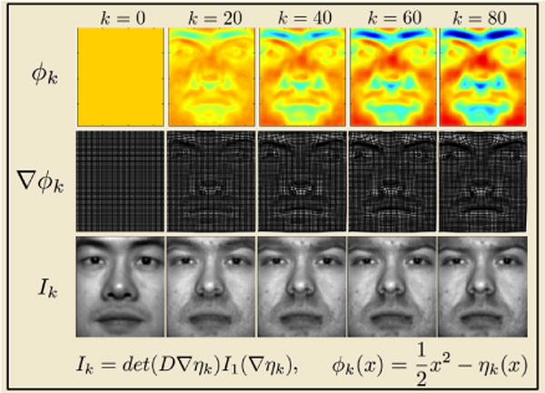
Visualization of the iterative update of the transport potential and correspondingly the transport displacement map through CWVP iterations.

D. Monge-Ampere equation

The Monge-Ampére partial differential equation (PDE) is defined as,

$$\det (H\varphi )=h(x,\varphi ,D\varphi )$$

for some functional h, and where Hϕ is the Hessian matrix of ϕ. The Monge-Ampére PDE is closely related to the Monge problem for the quadratic cost function. According to Bernier’s theorem (discussed in Section III-A3) when I₀ and I₁ are absolutely continuous PDFs defined on sets X, Y ⊂ ℝ^N, the optimal transport map that minimizes the 2-Wasserstein metric is uniquely characterized as the gradient of a convex function ϕ : X → Y. Moreover, we showed that the mass preserving constraint of the Monge problem can be written as det(D f)I₁(f) = I₀. Combining these results one can write,

$$\det (D(\nabla \varphi (x)))=\frac{I_0(x)}{I_1(\nabla \varphi ))}$$ (11)

where D∇ϕ = Hϕ, and therefore the equation shown above is in the form of the Monge-Ampére PDE. Now if ϕ is a convex function on X satisfying ∇ϕ(X) = Y and solving the Equation (11) then f^∗ = ∇ϕ is the optimal transportation map from I₀ to I₁. The geometrical constraint on this problem is rather unusual in PDEs and is often referred to as the optimal transport boundary conditions. Several authors have proposed numerical methods to obtain the optimal transport map through solving the Monge-Ampére PDE in Equation (11) [7, 33]. In particular the scheme in [7] is monotone, has compexity O(N) (up to logarithms) and is provably convergent. We conclude by remarking that several regularity results on the optimal transport maps were established through the Monge-Ampére equation (see [24] for references).

E. Semi-discrete approximation

Several works [31, 34] have considered the problem in which one PDF, I₀, has a continuous form while the other, I₁ is discrete, I₁(y) = Σq_iδ(y − y_i). It turns out that there exists weights w_i such that the optimal transport map f : X → Y can be described via a power diagram. More precisely the set of x mapping to y_i is the following cell of the power diagram:

$$P{D}_w(y_i)=\{x:{|x-y_i|}^2-w_i\le {|x-y_j|}^2-w_j,\forall j\}$$

The main observation is that the weights w_i are minimizers of the following unconstrained convex functional

$${\displaystyle \sum _i\left(q_i{w}_i-{\displaystyle \underset{P{D}_w(y_i)}{\int }({\Vert x-y_i\Vert }^2-w_i)I_0(x)dx}\right).}$$

Works by Mérigot [34], and Levy [31] use Newton based schemes and multiscale approaches to minimize the functional. The need to integrate over the power diagram makes the implementation somewhat geometrically delicate. Nevertheless recent implementation by Levy [31] gives impressive results in terms of speed. We also note that this approach provides the transportation mapping (not just the approximation of a plan).

V. Applications

In this section we review some recent applications of the optimal transport problem in signal and image processing, computer vision, and machine learning.

A. Image retrieval

One of the earliest applications of the optimal transport problem was in image retrieval. Rubner, Tomasi, and Guibas [44] employed the discrete Wasserstein metric, which they denoted as the Earth Mover’s Distance (EMD), to measure the dissimilarity between image signatures. In image retrieval applications, it is common practice to first extract features (i.e. color features, texture feature, shape features, etc.) and then generate high dimensional histograms or signatures (histograms with dynamic/adaptive binning), to represent images. The retrieval task then simplifies to finding images with similar representations (i.e. small distance between their histograms/signatures). The Wasserstein metric is specifically suitable for such applications as it can compare histograms/signatures of different sizes (histograms with different binning). This unique capability turns the Wasserstein metric into an attractive candidate in image retrieval applications [32, 44]. In [44], the Wasserstein metric was compared with common metrics such as the Jeffrey’s divergence, the χ² statistics, the L₁ distance, and the L₂ distance in an image retrieval task; and it was shown that the Wasserstein metric achieves the highest precision/recall performance amongst all.

Speed of computation is an important practical consideration in image retrieval applications. For almost a decade, the high computational cost of the optimal transport problem overshadowed its practicality in large scale image retrieval applications. Recent advancements in numerical methods including the work of Merigot [34], and Cuturi [14], among many others, have reinvigorated optimal transport-based distances as a feasible and appealing candidate for large scale image retrieval problems.

B. Registration and Morphing

Image registration deals with finding a common geometric reference frame between two or more images and it plays an important role in analyzing images obtained at different times or using different imaging modalities. Image registration and more specifically biomedical image registration is an active research area. Registration methods find a transformation f that maximizes the similarity between two or more image representations (e.g. image intensities, image features, etc.). Among the plethora of registration methods, nonrigid registration methods are especially important given their numerous applications in biomedical problems. They can be used to quantify the morphology of different organs, correct for physiological motion, and allow for comparison of image intensities in a fixed coordinate space (atlas). Generally speaking, nonrigid registration is a non-convex and non-symmetric problem, with no guarantee on existence of a globally optimal transformation.

Various work in the literature, deploy the Monge problem for image warping and elastic registration. Utilizing the Monge problem in an image warping/registration setting has a number of advantages. First, the existence and uniqueness of the global transformation (the optimal transport map) is known. Second, the problem is symmetric, meaning that the optimal transport map for warping I₀ to I₁ is the inverse of the optimal transport map for warping I₁ to I₀. Lastly, it provides a landmark-free and parameter-free registration scheme with a built-in mass preservation constraint. These advantages motivated several follow-up work to investigate the application of the Monge problem in image registration and warping [21, 22].

In addition to images, the optimal mass transport problem has also been used in point cloud and mesh registration [29] (see [24] for more references), which have various applications in shape analysis and graphics. In these applications, shape images (2D or 3D binary images) are first represented using either sets of weighted points (i.e. point clouds), using clustering techniques such as K-means or Fuzzy C-means, or with meshes. Then, a regularized variation of the optimal transport problem is solved to match such representations. The regularization on the transportation problem is often imposed to enforce the neighboring points (or vertices) to remain near to each other after the transformation.

C. Color transfer and texture synthesis

Texture mixing and color transfer are appealing applications of the optimal transport framework in image analysis, graphics, and computer vision. Here we briefly discuss these applications.

1) Color transfer

The purpose of color transfer is to change the color palette of an image to impose the feel and look of another image. Color transfer is generally performed through finding a map, which morphs the color distribution of the first image into the second one. For grayscale images, the color transfer problem simplifies to a histogram matching problem, which is solved through the one-dimensional optimal transport formulation [16]. In fact, the classic problem of histogram equalization is indeed a one-dimensional transport problem [16]. The color transfer problem, on the other hand, is concerned with pushing the three-dimensional color distribution of the first image into the second one. This problem can also be formulated as an optimal transport problem as demonstrated in [41] (see [24] for more references.).

A complication that occurs in the color transfer on real images, however, is that a perfect match between color distributions of the images is often not satisfying. This is due to the fact that a color transfer map may not transfer the colors of neighboring pixels in a coherent manner, and may introduce artifacts in the color transferred image. Therefore, the color transfer map is often regularized to make the transfer map spatially coherent [41]. Figure 7 shows a simple example of grayvalue and color transfer via optimal transport framework. It can be seen that the cumulative distribution of the grayvalue and color transferred images are similar to that of the input image.

Fig. 7.

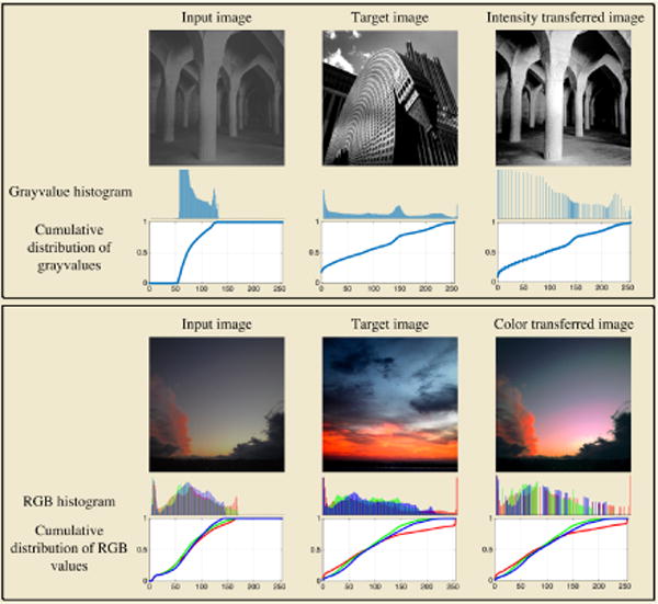
Grayvalue and color transfer via optimal transportation.

2) Texture synthesis and mixing

Texture synthesis is the problem of synthesizing a texture image that is visually similar to an exemplar input texture image, and has various applications in computer graphics and image processing. Many methods have been proposed for texture synthesis, among which are synthesis by recopy and synthesis by statistical modeling. Texture mixing, on the other hand, considers the problem of synthesizing a texture image from a collection of input texture images in a way that the synthesized texture provides a meaningful integration of the colors and textures of the input texture images. Metamorphosis is one of the successful approaches in texture mixing, which performs the mixing via identifying correspondences between elementary features (i.e. textons) among input textures and progressively morphing between the shapes of elements. In other approaches, texture images are first parametrized through a tight frame (often steerable wavelets) and statistical modeling is performed on the parameters.

Other successful approaches include the random phase and spot noise texture modeling [18], which model textures as stationary Gaussian random fields. Briefly, these methods are based on the assumption that the visual texture perception is based on the spectral magnitude of the texture image. Therefore, utilizing the spectral magnitude of an input image and randomizing its phase will lead to a new synthetic texture image which is visually similar to the input image. Ferradans et al. [18] utilized this assumption together with the Wasserstein geodesics to interpolate between spectral magnitude of texture images, and provide synthetic mixed texture images. Figure 8 shows an example of texture missing via the Wasserstein geodesic between the spectral magnitudes of the input texture images. The in-between images are synthetically generated using the random phase technique.

Fig. 8.

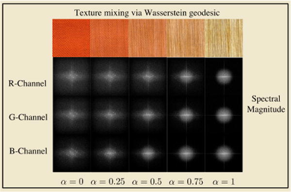
An example of texture mixing via optimal transport using the method presented in Ferradans et al. [18]

D. Image denoising and restoration

The optimal transport problem has also been used in several image denoising and restoration problems [30]. The goal in these applications is to restore or reconstruct an image from noisy or incomplete observation. Lellmann et al. [30] utilized the Kantorovich-Rubinsten discrepancy term together with a Total Variation term in the context of image denoising. They called their method Kantorovich-Rubinstein-TV (KR-TV) denoising. It should be noted that, the Kantorovich-Rubinstein metric is closely related to the 1-Wasserstein metric (for one dimensional signals they are equivalent). The KR term in their proposed functional provides a fidelity term for denoising while the TV term enforces a piecewise constant reconstruction.

E. Transport based morphometry

Given their suitability for comparing mass distributions, transport-based approaches for performing pattern recognition of morphometry encoded in image intensity values have also recently emerged. Recently described approaches for transport-based morphometry (TBM) [4, 27, 50] work by computing transport maps or plans between a set of images and a reference or template image. The transport plans/maps are then utilized as an invertible feature/transform onto which pattern recognition algorithms such as principal component analysis (PCA) or linear discriminant analysis (LDA) can be applied. In effect, it utilizes the LOT framework described earlier in Section III-C1. These techniques has been recently employed to decode differences in cell and nuclear morphology for drug screening [4], and cancer detection histopathology [39] and cytology images amongst other applications including the analysis of galaxy morphologies [27], for example.

Deformation-based methods have long been used in analyzing biomedical images. TBM, however, is different from those deformation-based methods in that it has numerically exact, uniquely defined solutions for the transport plans or maps used. That is, images can be matched with little perceptible error. The same is not true in methods that rely on registration via the computation of deformations, given the significant topology differences commonly found in medical images. Moreover, TBM allows for comparison of the entire intensity information present in the images (shapes and textures), while deformation-based methods are usually employed to deal with shape differences. Figure 9 shows a schematic of the TBM steps applied to a cell nuclei dataset. It can be seen that the TBM is capable of modeling the variation in the dataset. In addition, it enables one to visualize the classifier, which discriminates between image classes (in this case malignant versus benign).

Fig. 9.

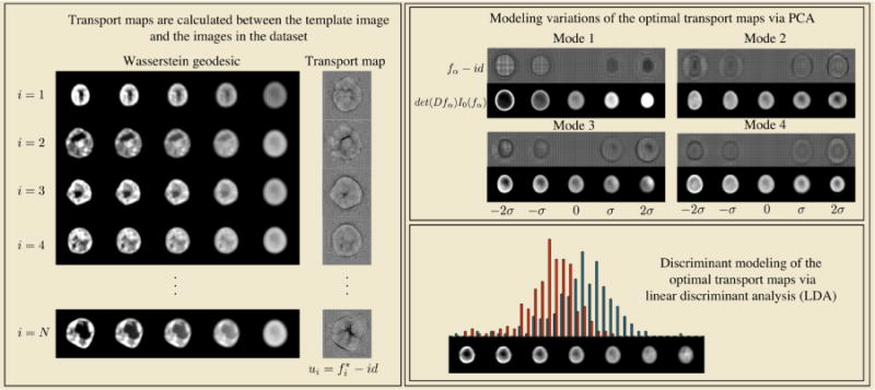
The schematic of the TBM framework. The optimal transport maps between input images I₁, …, I_N and a template image I₀ is calculated. Next, linear statistical modeling such as principal component analysis (PCA), linear discriminant analysis (LDA), and canonical correlation analysis (CCA) is performed on the optimal transport maps. The resulting transport maps obtained from the statistical modeling step are then applied to the template image to visualize the results of the analysis in the image space.

F. Super-Resolution

Super-resolution is the process of reconstructing a high-resolution image from one or several corresponding low-resolution images. Super-resolution algorithms can be broadly categorized into two major classes namely “multi-frame” super resolution and “single-frame” super resolution, based on the number of low-resolution images they require to reconstruct the corresponding high-resolution image. The transport-based morphometry approach was used for single frame super resolution in [26] to reconstruct high-resolution faces from very low resolution input face images. The authors utilized the transport-based morphometry in combination with subspace learning techniques to learn a nonlinear model for the high-resolution face images in the training set.

In short, the method consists of a training and a testing phase. In the training phase, it uses high resolution face images and morphs them to a template high-resolution face through optimal transport maps. Next, it learns a subspace for the calculated optimal transport maps. A transport map in this subspace can then be applied to the template image to synthesize a high-resolution face image. In the testing phase, the goal is to reconstruct a high-resolution image from the low-resolution input image. The method searches for a synthetic high-resolution face image (generated from the transport subspace) that provides a corresponding low-resolution image which is similar to the input low-resolution image. Figure 10 shows the steps used in this method and demonstrates reconstruction results.

Fig. 10.

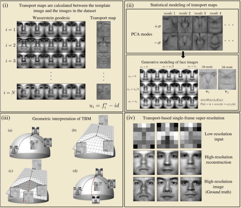
In the training phase, optimal transport maps that morph the template image to high-resolution training face images are calculated (i). Principal component analysis (PCA) is used to learn a linear subspace for transport maps for which a linear combination of obtained eigenmaps can be applied to the template image to obtain synthetic face images (ii). A geometric interpretation of the problem is depicted in panel (iii), and reconstruction results are shown in panel (iv).

G. Machine-Learning and Statistics

The optimal transport framework has recently attracted ample attention from the machine learning and statistics communities [12, 19, 25, 28, 36]. Some applications of the optimal transport in these arenas include various transport-based learning methods [19, 28, 36, 48], domain adaptation, Bayesian inference [12, 13], and hypothesis testing [15, 42] among others. Here we provide a brief overview of the recent developments of transport-based methods in machine learning and statistics.

1) Learning

Transport-based distances have been recently used in several works as a loss function for regression, classification, etc. Montavon, Müller, and Cuturi [36] for instance utilized the dual formulation of the entropy regularized Wasserstein distance to train restricted Boltzmann machines (RBMs). Boltzmann machines are probabilistic graphical models (Markov random fields) that can be categorized as stochastic neural networks and are capable of extracting hierarchical features at multiple scales. RBMs are bipartite graphs which are special cases of Boltzmann machines, which define parameterized probability distributions over a set of d-binary input variables (observations) whose states are represented by h binary output variables (hidden variables). RBMs’ parameters are often learned through information theoretic divergences such as KL-Divergence. Montavon et al. [36] proposed an alternative approach through a scalable entropy regularized Wasserstein distance estimator for RBMs, and showed the practical advantages of this distance over the commonly used information divergence-based loss functions.

In another approach, Frogner et al. [19] used the entropy regularized Wasserstein loss for multi-label classification. They proposed a relaxation of the transport problem to deal with unnormalized measures by replacing the equality constraints in Equation (6) with soft penalties with respect to KL-divergence. In addition, Frogner et al. [19] provided statistical bounds on the expected semantic distance between the prediction and the groundtruth. In yet another approach, Kolouri et al. [28] utilized the sliced Wasserstein metric and provided a family of positive definite kernels, denoted as Sliced-Wasserstein Kernels, and showed the advantages of learning with such kernels. The Sliced-Wasserstein Kernels were shown to be effective in various machine learning tasks including classification, clustering, and regression.

Solomon et al. [48] considered the problem of graph-based semi-supervised learning, in which graph nodes are partially labeled and the task is to propagate the labels throughout the nodes. Specifically, they considered a problem in which the labels are histograms. This problem arises for example in traffic density prediction, in which the traffic density is observed for a few stop lights over 24 hours in a city and the city is interested in predicting the traffic density in the un-observed stop lights. They pose the problem as an optimization of a Dirichlet energy for distribution-valued maps based on the 2-Wasserstein distance, and present a Wasserstein propagation scheme for semi-supervised distribution propagation along graphs.

More recently, Arjovskly et al. [3] compared various distances, namely total variation, KL divergence, Jenson-Shannon divergence, and the Wasserstein distance in training generative adversarial networks (GAN). They demonstrated (theoretically and numerically) that the Wasserstein distance leads to a superior performance compared to the later dissimilarity measures. They specifically showed that, their proposed Wasserstein GAN does not suffer from common issues in such networks, including instability and mode collapse.

2) Domain adaptation

Domain adaptation is one of the fundamental problems in machine learning which has gained proper attention from the machine learning research community in the past decade. Domain adaptation is the task of transfer ring knowledge from classifiers trained on available labeled data to unlabeled test domains with data distributions that differ from that of the training data. The optimal transport framework is recently presented as a potential major player in domain adaptation problems [12, 13]. Courty, Flamary, and Davis [12], for instance, assumed that there exists a non-rigid transformation between the source and target distributions and find this transformation using an entropy regularized optimal transport problem. They also proposed a label-aware version of the problem in which the transport plan is regularized so a given target point (testing exemplar) is only associated with source points (training exemplars) belonging to the same class. Courty et al. [12] showed that domain adaptation via regularized optimal transport outperform the state-of-the-art results in several challenging domain adaptation problems.

3) Bayesian inference

Another interesting and emerging application of the optimal transport problem is in Bayesian inference [17]. In Bayesian inference, one critical step is the evaluation of expectations with respect to a posterior probability function, which leads to complex multidimensional integrals. These integrals are commonly solved through the Monte Carlo numerical integration, which requires independent sampling from the posterior distribution. In practice, sampling from a general posterior distribution might be difficult, therefore the sampling is performed via a Markov Chain which converges to the posterior probability after a certain number of steps. This leads to the celebrated Markov Chain Monte Carlo (MCMC) method. The downside of MCMC is that the samples are not independent and hence the convergence of the empirical expectation is slow. El Moselhy and Marzouk [17] proposed a transport-based method that evades the need for Markov chain simulation by allowing direct sampling from the posterior distribution. The core idea in their work is to find a transport map (via a regularized Monge formulation), which pushes forward the prior measure to the posterior measure. Then, sampling the prior distribution and applying the transport map to the samples, will lead to a sampling scheme from the posterior distribution. Figure 11 shows the basic idea behind these methods.

Fig. 11.

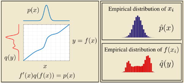
Left panel shows the prior distribution p and the posterior distribution q and the corresponding transport map f that pushes p into q. One million samples, x_i, were generated from distribution p and the top-right panel shows the empirical distribution of these samples denoted as $\widehat{p}$. The bottom-right panel shows the empirical distribution of transformed samples, y_i = f (x_i), denoted as $\widehat{q}$.

4) Hypothesis testing

Wasserstein distance is used for goodness of fit testing in [15] and for two sample testing in [42]. Ramdas et al. [42] presented connections between the entropy regularized Wasserstein distance, multivariate Energy distance, and the kernel maximum mean discrepancy (MMD), and provided a “distribution free” univariate Wasserstein test statistic. These and other applications of transport-related concepts show the promise of the mathematical modeling technique in the design of statistical data analysis methods to tackle modern learning problems.

Finally, we note that in the interest of brevity, a number of other important applications of transport-related techniques were not discussed above, but are certainly interesting on their own right. For a more detailed discussion and more references please refer to [24].

VI. Summary and Conclusions

Transport-related methods and applications have come a long way. While earlier applications focused primarily in civil engineering and economics problems, they have recently begun to be employed in a wide variety of problems related to signal and image analysis, and pattern recognition. In this tutorial, seven main areas of application were reviewed: image retrieval V-A, registration and morphing V-B, color transfer and texture analysis V-C, image restoration V-D, transport-based morphometry V-E, image super-resolution V-F, and machine learning and statistics V-G. Transport and related techniques have received increased attention in recent years. Overall, researchers have found that the application of transport-related concepts can be helpful to solve problems in diverse applications. Given recent trends, it seems safe to expect that the number of different application areas will continue to grow.

In its most general form, the transport-related techniques reviewed in this tutorial can be thought as mathematical models for signals, images, and in general data distributions. Transport-related metrics involve calculating differences not only of pixel or distribution intensities, but also “where” they are located in the corresponding coordinate space (a pixel coordinate in an image, or a particular axis in some arbitrary feature space). As such, the geometry (e.g. geodesics) induced by such metrics can give rise to dramatically different algorithms and data interpretation results. The interesting performance improvements recently obtained could motivate the search for a more rigorous mathematical understanding of transport-related metrics and applications.

We note that the emergence of numerically precise and efficient ways of computing transport-related metrics and geodesics, presented in section IV also serves as an enabling mechanism. Coupled with the fact that several mathematical properties of transport-based metrics have been extensively studied, we believe that the ground is set for their increased use as foundational tools or building blocks based on which complex computational systems can be built. The confluence of these emerging ideas may spur a significant amount of innovation in a world where sensor and other data is becoming abundant, and computational intelligence to analyze these is in high demand. We believe transport-based models while become an important component of the ever expanding tool set available to modern signal processing and data science experts.

Biographies

Soheil Kolouri received his B.S. degree in electrical engineering from Sharif University of Technology, Tehran, Iran, in 2010, and his M.S. degree in electrical engineering in 2012 from Colorado State University, Fort Collins, Colorado. He earned his doctorate degree in biomedical engineering from Carnegie Mellon University in 2015. His thesis, titled, “Transport-based pattern recognition and image modeling”, won the best thesis award. He is currently at HRL Laboratories, Malibu, California, United States.

Serim Park received her B.S. degree in Electrical and Electronic Engineering from Yonsei University, Seoul, Korea in 2011 and is currently a doctoral candidate in the Electrical and Computer Engineering Department at Carnegie Mellon University, Pittsburgh, United States. She is mainly interested in signal processing and machine learning, especially designing new signal and image transforms and developing novel systems for pattern recognition.

Matthew Thorpe received his BSc, MSc and PhD in Mathematics from the University of Warwick, UK in 2009, 2012 and 2015 respectively and his MScTech in Mathematics from the University of New South Wales, Australia, in 2010. He is currently a postdoctoral associate within the mathematics department at Carnegie Mellon University.

Dejan Slepčev earned B.S degree in mathematics from the University of Novi Sad in 1995, M.A. degree in mathematics from University of Wisconsin Madison in 2000 and Ph.D. in mathematics from University of Texas at Austin in 2002. He is currently associate professor at the Department of Mathematical Sciences at Carnegie Mellon University.

Gustavo K. Rohde earned B.S. degrees in physics and mathematics in 1999, and the M.S. degree in electrical engineering in 2001 from Vanderbilt University. He received a doctorate in applied mathematics and scientific computation in 2005 from the University of Maryland. He is currently an associate professor of Biomedical Engineering, and Electrical and Computer Engineering at the University of Virginia. Contact: gustavo@virginia.edu.

References

- 1.Ambrosio L, Gigli N, Savaré G. Lectures in Mathematics ETH Zürich. second. Birkhäuser Verlag; Basel: 2008. Gradient flows in metric spaces and in the space of probability measures. [Google Scholar]
- 2.Angenent S, Haker S, Tannenbaum A. Minimizing flows for the Monge–Kantorovich problem. SIAM journal on mathematical analysis. 2003;35(1):61–97. [Google Scholar]
- 3.Arjovsky M, Chintala S, Bottou L. Wasserstein gan. 2017 arXiv preprint arXiv:1701.07875. [Google Scholar]
- 4.Basu S, Kolouri S, Rohde GK. Detecting and visualizing cell phenotype differences from microscopy images using transport-based morphometry. Proceedings of the National Academy of Sciences. 2014;111(9):3448–3453. doi: 10.1073/pnas.1319779111. [DOI] [PMC free article] [PubMed] [Google Scholar]
- 5.Benamou JD, Brenier Y. A computational fluid mechanics solution to the Monge-Kantorovich mass transfer problem. Numerische Mathematik. 2000;84(3):375–393. [Google Scholar]
- 6.Benamou JD, Carlier G, Cuturi M, Nenna L, Peyré G. Iterative Bregman projections for regularized transportation problems. SIAM Journal on Scientific Computing. 2015;37(2):A1111–A1138. [Google Scholar]
- 7.Benamou JD, Froese BD, Oberman AM. Numerical solution of the optimal transportation problem using the Monge-Ampére equation. Journal of Computational Physics. 2014;260:107–126. [Google Scholar]
- 8.Bonneel N, Rabin J, Peyré G, Pfister H. Sliced and Radon Wasserstein barycenters of measures. Journal of Mathematical Imaging and Vision. 2015;51(1):22–45. [Google Scholar]
- 9.Brenier Y. Polar factorization and monotone rearrangement of vector-valued functions. Communications on Pure and Applied Mathematics. 1991;44(4):375–417. [Google Scholar]
- 10.Caffarelli LA. The regularity of mappings with a convex potential. Journal of the American Mathematical Society, pages. 1992:99–104. [Google Scholar]
- 11.Chartrand R, Vixie K, Wohlberg B, Bollt E. A gradient descent solution to the Monge-Kantorovich problem. Applied Mathematical Sciences. 2009;3(22):1071–1080. [Google Scholar]
- 12.Courty N, Flamary R, Tuia D. Machine Learning and Knowledge Discovery in Databases. Springer; 2014. Domain adaptation with regularized optimal transport; pp. 274–289. [Google Scholar]
- 13.Courty N, Flamary R, Tuia D, Rakotomamonjy A. Optimal transport for domain adaptation. 2015 doi: 10.1109/TPAMI.2016.2615921. arXiv preprint arXiv:1507.00504. [DOI] [PubMed] [Google Scholar]
- 14.Cuturi M. Sinkhorn distances: Lightspeed computation of optimal transport. Advances in Neural Information Processing Systems. 2013:2292–2300. [Google Scholar]
- 15.del Barrio E, Cuesta-Albertos JA, Matrán C, et al. Tests of goodness of fit based on the l_2-Wasserstein distance. The Annals of Statistics. 1999;27(4):1230–1239. [Google Scholar]
- 16.Delon J. Midway image equalization. Journal of Mathematical Imaging and Vision. 2004;21(2):119–134. [Google Scholar]
- 17.El Moselhy TA, Marzouk YM. Bayesian inference with optimal maps. Journal of Computational Physics. 2012;231(23):7815–7850. [Google Scholar]
- 18.Ferradans S, Xia GS, Peyré G, Aujol JF. Static and dynamic texture mixing using optimal transport. Springer; 2013. [Google Scholar]
- 19.Frogner C, Zhang C, Mobahi H, Araya M, Poggio TA. Learning with a Wasserstein loss. Advances in Neural Information Processing Systems. 2015:2044–2052. [Google Scholar]
- 20.Gangbo W, McCann RJ. The geometry of optimal transportation. Acta Mathematica. 1996;177(2):113–161. [Google Scholar]
- 21.Haber E, Rehman T, Tannenbaum A. An efficient numerical method for the solution of the l2 optimal mass transfer problem. SIAM Journal on Scientific Computing. 2010;32(1):197–211. doi: 10.1137/080730238. [DOI] [PMC free article] [PubMed] [Google Scholar]
- 22.Haker S, Zhu L, Tannenbaum A, Angenent S. Optimal mass transport for registration and warping. International Journal of Computer Vision. 2004;60(3):225–240. [Google Scholar]
- 23.Kantorovich LV. On translation of mass (in Russian), C R. Doklady. Acad Sci USSR. 1942;37:199–201. [Google Scholar]
- 24.Kolouri S, Park S, Thorpe M, Slepčev D, Rohde GK. Transport-based analysis, modeling, and learning from signal and data distributions. 2016 arXiv preprint arXiv:1609.04767. [Google Scholar]
- 25.Kolouri S, Park SR, Rohde GK. The Radon cumulative distribution transform and its application to image classification. Image Processing, IEEE Transactions on. 2016;25(2):920–934. doi: 10.1109/TIP.2015.2509419. [DOI] [PMC free article] [PubMed] [Google Scholar]
- 26.Kolouri S, Rohde GK. Transport-based single frame super resolution of very low resolution face images. Proceedings of the IEEE Conference on Computer Vision and Pattern Recognition. 2015:4876–4884. [Google Scholar]
- 27.Kolouri S, Tosun AB, Ozolek JA, Rohde GK. A continuous linear optimal transport approach for pattern analysis in image datasets. Pattern Recognition. 2016;51:453–462. doi: 10.1016/j.patcog.2015.09.019. [DOI] [PMC free article] [PubMed] [Google Scholar]
- 28.Kolouri S, Zou Y, Rohde GK. Sliced Wasserstein kernels for probability distributions. The IEEE Conference on Computer Vision and Pattern Recognition (CVPR) 2016 Jun; [Google Scholar]
- 29.Lai R, Zhao H. Multi-scale non-rigid point cloud registration using robust sliced-Wasserstein distance via Laplace-Beltrami eigenmap. 2014 arXiv preprint arXiv:1406.3758. [Google Scholar]
- 30.Lellmann J, Lorenz DA, Schönlieb C, Valkonen T. Imaging with Kantorovich–Rubinstein discrepancy. SIAM Journal on Imaging Sciences. 2014;7(4):2833–2859. [Google Scholar]
- 31.Lévy B. A numerical algorithm for L2 semi-discrete optimal transport in 3D. ESAIM Math Model Numer Anal. 2015;49(6):1693–1715. [Google Scholar]
- 32.Li P, Wang Q, Zhang L. A novel earth mover’s distance methodology for image matching with gaussian mixture models. Proceedings of the IEEE International Conference on Computer Vision. 2013:1689–1696. [Google Scholar]
- 33.Loeper G, Rapetti F. Numerical solution of the Monge–ampère equation by a newton’s algorithm. Comptes Rendus Mathematique. 2005;340(4):319–324. [Google Scholar]
- 34.Mérigot Q. A multiscale approach to optimal transport. Computer Graphics Forum. 2011;30(5):1583–1592. [Google Scholar]
- 35.Monge G. Mémoire sur la théorie des déblais et des remblais. De l’Imprimerie Royale; 1781. [Google Scholar]
- 36.Montavon G, Müller KR, Cuturi M. Wasserstein training of Boltzmann machines. 2015 arXiv preprint arXiv:1507.01972. [Google Scholar]
- 37.Oberman AM, Ruan Y. An efficient linear programming method for optimal transportation. 2015 arXiv preprint arXiv:1509.03668. [Google Scholar]
- 38.Otto F. The geometry of dissipative evolution equations: the porous medium equation. Communications in Partial Differential Equations. 2001;26(1–2):101–174. [Google Scholar]
- 39.Ozolek JA, Tosun AB, Wang W, Chen C, Kolouri S, Basu S, Huang H, Rohde GK. Accurate diagnosis of thyroid follicular lesions from nuclear morphology using supervised learning. Medical image analysis. 2014;18(5):772–780. doi: 10.1016/j.media.2014.04.004. [DOI] [PMC free article] [PubMed] [Google Scholar]
- 40.Park SR, Kolouri S, Kundu S, Rohde GK. The cumulative distribution transform and linear pattern classification. Applied and Computational Harmonic Analysis. 2017 [Google Scholar]
- 41.Rabin J, Ferradans S, Papadakis N. Image Processing (ICIP), 2014 IEEE International Conference on. IEEE; 2014. Adaptive color transfer with relaxed optimal transport; pp. 4852–4856. [Google Scholar]
- 42.Ramdas A, Garcia N, Cuturi M. On Wasserstein two sample testing and related families of nonparametric tests. 2015 arXiv preprint arXiv:1509.02237. [Google Scholar]
- 43.Rohde GK, et al. Transport and other Lagrangian transforms for signal analysis and discrimination. http://faculty.virginia.edu/rohde/transport.
- 44.Rubner Y, Tomasi C, Guibas LJ. The earth mover’s distance as a metric for image retrieval. International Journal of Computer Vision. 2000;40(2):99–121. [Google Scholar]
- 45.Santambrogio F. Optimal transport for applied mathematicians. Springer; 2015. [Google Scholar]
- 46.Schmitzer B. Scale Space and Variational Methods in Computer Vision. Springer; 2015. A sparse algorithm for dense optimal transport; pp. 629–641. [Google Scholar]
- 47.Solomon J, de Goes F, Studios PA, Peyré G, Cuturi M, Butscher A, Nguyen A, Du T, Guibas L. Convolutional Wasserstein distances: Efficient optimal transportation on geometric domains. ACM Transactions on Graphics (Proc SIGGRAPH 2015) 2015 to appear. [Google Scholar]
- 48.Solomon J, Rustamov R, Guibas L, Butscher A. Wasserstein propagation for semi-supervised learning. Proceedings of The 31st International Conference on Machine Learning. 2014:306–314. [Google Scholar]
- 49.Villani C. Optimal transport: old and new. Vol. 338. Springer Science & Business Media; 2008. [Google Scholar]
- 50.Wang W, Slepcev D, Basu S, Ozolek JA, Rohde GK. A linear optimal transportation framework for quantifying and visualizing variations in sets of images. International journal of computer vision. 2013;101(2):254–269. doi: 10.1007/s11263-012-0566-z. [DOI] [PMC free article] [PubMed] [Google Scholar]