

Abstract
Here, a method based on viscosity-type regularization is proposed for magnetic resonance electrical property tomography (MREPT) to mitigate persistent artifacts when it is used to reconstruct a map of electrical properties based on data from a magnetic resonance imaging scanner. The challenges for solving the corresponding partial differential equation (PDE) are discussed in detail. The existing artifacts in the numerical results are pointed out and classified. The methods in the literature for MREPT are mainly based on an assumption of local homogeneity, which makes the approach simple but leads to artifacts in the transition region where electrical properties vary rapidly. Recent work has focused on eliminating the assumption of local homogeneity, and one of the solutions is convection–reaction MREPT that is based on a first-order PDE. Numerical solutions of the PDE have persistent artifacts in certain regions and global spurious oscillations. Here, a method based on viscosity-type regularization is proposed to effectively mitigate the aforementioned problems. Finite difference method is used for discretizing the governing PDE. Numerical experiments are presented to analyze the problem in detail. Electrical properties of different phantoms are successfully retrieved. The efficiency, accuracy, and noise tolerance of the proposed method are illustrated with numerical results.
Keywords: magnetic resonance, electrical property tomography, magnetic resonance safety, radio frequency field, partial differential equation, inverse problem
Introduction
Magnetic resonance imaging (MRI)-based magnetic resonance electrical property tomography (MREPT) (1, 2) is a strategy for noninvasively reconstructing electrical properties (EPs) (permittivity and electrical conductivity) of the human body without using additional hardware to a magnetic resonance (MR) scanner. It has been intensively developed in recent years for reconstructing the EPs of human tissues based on the measurable data (radiofrequency [RF] field distribution called B1-map) (3) from an MRI scanner because the B1-field carries the information of EP distribution in the human body.
MREPT is an important technology in various areas in medicine and biology. The constructed EP map can show the anatomical structure of the human body by the high contrast of EPs between different tissues (4). Cancerous tissues, including those at the early stages, are highly distinguishable from healthy ones (5, 6). Therefore, the EP map provides a good tool for early cancer detection. It can also provide guidance to design body-centric communications (7) and electromagnetics-based therapies (8). EP maps can also help in understanding the activities of cells, in particular with exposure to either static or dynamic electromagnetic waves (9). Moreover, an EP map is crucial for accurate calculation of specific absorption rate, which is a main parameter for assessing the risk of RF and microwave radiation and that of ultrahigh-field MRI scanning (10, 11).
MREPT was originally proposed by Haacke et al. (12) and first implemented by Wen (13). The Helmholtz equation for homogeneous material was proposed for calculating both conductivity and permittivity with positively circularly polarized component of the magnetic field (), which corresponds to the RF transmit field. Another MREPT method was developed and systematically studied by Katscher et al. (14) and Voigt et al. (15). The integral forms of Faraday's law and Ampère's law were applied to formulate the governing equation based on . However, these methods are based on an assumption of local homogeneity for simplification. This assumption leads to artifacts in the region where EPs vary either quickly or abruptly (3, 16, 17). The reconstruction errors are rigorously analyzed by Seo et al. (18). A recent work was focused on removing the local homogeneity assumption (19).
One full generalization of these methods was performed by Sodickson et al., and the technique was named Local Maxwell Tomography (LMT) (20, 21). The governing equation of this method was derived from Faraday's law and Ampère's law. The unmeasurable magnetic field components are eliminated by using Gauss's law. The method is physically feasible and free of assumptions. Magnetic fields measured using an MRI scanner with multiple channels are used to solve the unknown. Although the assumption of local homogeneity is removed in LMT, higher-order partial differentiation over the magnetic field is needed in the calculation, which significantly increases this method's sensitivity to noise.
Another MREPT method (22) was proposed on the basis of the fact that the magnetic field near the center of a birdcage or a transverse electromagnetic coil is homogeneous along its central axis (23, 24), and it is assumed that the contribution of the along-axis component of the magnetic field is negligible when the region of interest is close to the center of the coil. A first-order PDE including a gradient term of the unknown EP was formulated via properly manipulating Maxwell equations, and the gradient term describes the inhomogeneity of the object under investigation. This method is more general than the MREPT proposed by Katscher et al. (14) and has a simpler form than LMT.
Hafalir et al. (25) then named this method as convection–reaction MREPT (cr-MREPT), as its governing equation is similar to the convection–reaction equation (26). The first-order PDE was then solved by Hafalir et al. (25) for 2-dimensional reconstruction using a strong form with finite element method (FEM) (27). An obvious artifact was observed in the region where the gradient of is close to zero. Although 2 methods, the double-excitation and the constraint MREPT, were further proposed by Hafalir et al. (25) to improve the results, artifacts reappear when noise exists. Meanwhile, cr-MREPT does not work with every phantom. Even with the phantoms used by the authors, the reconstructed EPs deviate seriously from the true values in a large region close to the central artifact. High sensitivity of noise was also observed.
In parallel with the work of Hafalir et al., Ammari et al. (19) also attempted to solve this PDE via an adjoint-based iterative reconstruction algorithm. The real and imaginary parts of the equation are separated to produce a coupled equation pair solved by the iterative scheme. This method can construct a blur image of the EPs without the aforementioned artifacts, but it is not applicable in the region where the gradient of field is close to zero, and the produced linear system is ill-conditioned. The method also converges slower than the FEM-based method (19).
The solution of the first-order PDE shows persistent artifacts where approaches zero. Other than that, global spurious oscillations exist in the solution of this first-order PDE. Therefore, directly solving it with numerical methods is difficult. Here, the existing challenges for solving the PDE are discussed in detail. The existing artifacts in the numerical results are pointed out and classified. An effective viscosity-type regularization (28) solution is applied to mitigate the aforementioned problems. A Laplacian term is introduced into the first-order PDE for stabilizing the entire system, which can be solved by either the finite difference (FD) method or FEM. The governing PDE is in the first order, so its solution will be a linear function that depends on the space coordinates, and it can present sharp variations in space. Because the PDE is not a singularly disturbed equation (29, 26, 30), the introduced second-order Laplacian term will modify the PDE to obtain a second-order solution, which is an approximation of its exact solution and presents a smoother property in space.
The derivation of the formulation is briefly presented for the convenience of discussion; behaviors of the equation are analyzed in detail before introducing the viscosity-type regularization. Numerical experiments are used to facilitate the analysis of the existing problems and to show the effectiveness of the proposed approach. Finite difference method is applied for discretization. The proposed method is applied for reconstructing the EPs of different phantoms. Accuracy, stability, and noise tolerance of the method are illustrated with numerical results.
Theory and Methodology
The governing PDE for cr-MREPT are given as follows:
| (1) |
This equation can be solved for reconstructing EPs of a 3-dimensional object (see online supplemental Appendix for the relating derivation of this equation). If γ does not vary severely along the z direction, becomes negligible. Equation (1) is then simplified as follows for a single section located at the center of birdcage coil:
| (2) |
and are vectors and without the z-component, respectively.
. Notice that still needs to be evaluated in a 3-dimensional form. Magnetic field Hz is not measurable using MRI, but its contribution is negligible compared with , as Hz is generally close to zero in the center of the birdcage coil. Therefore equation (2) could be further simplified as follows:
| (3) |
For homogeneous regions, ; therefore, equation (3) can be simplified as , which is the governing equation proposed by Haacke et al. and Wen (12, 13), named, in this content, standard MREPT (stdMREPT).
Therefore, the original inverse problem equivalently becomes a problem of solving the first-order PDE (3). It has the form of a stationary convection–reaction equation, which is a mathematical model for fluid dynamics (31). Thus, the MREPT based on equation (3) is called cr-MREPT by Hafalir et al. (25).
The coefficients of PDE (3) are complex, making the PDE exhibit different mathematical and numerical behaviors from the stationary convection–reaction equations that have real coefficients. In particular, both equations show global spurious oscillations in their solutions (26). For convection–reaction equations (real coefficients), these global spurious oscillations are caused by the mesh density for discretization, and the results converge better when the mesh size decreases. However, this fact does not hold for equation (3), where the coefficients are complex. Instead, the spurious oscillation in equation (3) is caused by a fundamental mathematical drawback of itself; this is further discussed as follows.
Equation (3) can be reformed as follows:
| (4) |
with and . According to the Cauchy–Kowalevski theorem (32), a necessary condition for equation (4) to have a smooth solution is that is analytic in region Ω (19). However, is not smooth in the region where electrical parameters vary rapidly (as in Figure 3H for a 2-layer cylindrical phantom with difference and σ in different layers). Discontinuity of exists at the boundary where electrical parameters vary rapidly. Therefore, a smooth solution of σ and cannot be obtained with equation (3), and a better strategy is needed for good numerical stability, accuracy, and efficiency.
Figure 3.

σ (A) and (B) of phantom shown in Figure 2 are reconstructed by applying convection–reaction magnetic resonance electrical property tomography (MREPT) (cr-MREPT) based on equation (3). σ (C) and (D) reconstructed using equation (2). Real (E) and imaginary (F) parts of , absolute value of (G) and (H), are also presented.
Here, a viscosity-type regularization method (28) is applied to equation (3) to eliminate the global spurious oscillation in its solution. The governing equation becomes the following equation:
| (5) |
where is the additional Laplacian term, and ρ is a constant that is always <1 but >0. This approach does not lead to a singularly disturbed problem (29, 26, 30). The additional Laplacian term plays a regularization role. This stabilized MREPT method is named as stabMREPT. There is no good way for deciding the optimum value of ρ yet, but it can be chosen as several times or a fraction of the maximum of , which is the x-component of . There are 2 ways to add the Laplacian term. One is adding it to the whole calculation domain, as shown in equation (5), and the other is adding it to the region where it is necessary (33) to produce more accurate results, but the optimal coefficients of the added Laplacian term need to be determined in a complex way, rendering it complicated. Here, only equation (5) is implemented for showing the idea. Central difference formula of the FD method is used for discretization.
Discretization Strategy
A square domain denoted as Ω and bounded by is discretized by small squares with and grid points along the x and y directions, respectively, giving data points in space. and are the step lengths along x and y directions, respectively. Use i and j to index the mesh points along x and y with and j := , respectively. The values of and γ at the point (i, j) are represented as and , respectively.
Allowing with and . The values of and at point (i, j) are represented with and , respectively. Using first-order central difference formula, and are given as follows:
| (6) |
| (7) |
Here, the imaginary unit i can be easily distinguished from the index i on the basis of its location. Representing the data of at the point (i, j) as , the second-order central difference formula is used to discretize , which gives the following equation:
| (8) |
k is the index for sections along the z-direction. Two extra sections at and away from the central section are used to calculate the partial differentiation of over z.
Another way for calculating , and is by using the Savitzky–Golay (SG) filter (34), which has been widely used to smooth noisy data. Here, is approximated with the following equation:
| (9) |
where (x, y) is the corresponding coordinate of . ap, p = 1, . ., 6 are polynomial coefficients, which need to be decided with the measured data of . As an example, at mesh grid point (i, j), has 8 neighbors, as shown in Figure 1. These neighbors or itself could be used for interpolation with Stanley et al. (9), which will produce an overfitting linear system about the unknown coefficients ap, p = 1, …, 6. A least-square method could then be used for solving the unknown.
Figure 1.

Neighbors of in a mesh grid.
The derivatives over at the point (i, j) are then calculated using the following equations:
| (10) |
| (11) |
| (12) |
Here, (xi, yj) is the coordinate of the grid point (i, j). Notice that the Laplacian term over includes the second-order partial differentiation of over z, which is calculated with a central difference formula, with the data at sections located at and . With equations (6)–(8), or (10)–(12), equation (5) can be easily discretized with the first- and second-order central difference formula, as follows:
| (13) |
A linear system is produced via assembling (13) for all points indexed by (i, j). The linear system is denoted as . The sparsity of the tridiagonal matrix allows efficient calculation with Gaussian elimination. The Dirichlet boundary condition is assumed here. Vector g represents the unknowns . The relative permittivity and conductivity at (i, j) can be calculated based on the real and imaginary parts of .
Numerical Experiments
In the calculation, as input is simulated with FEM-based software COMSOL (35). A 16-leg high-pass shielded birdcage coil with a radius of 14.5 cm and a leg-length of 24 cm (36) is built to work at 127.74 MHz (3 T MRI system) to produce a homogeneous within the coil, and it is placed with its axis along the z-axis. The coil is driven by 2 ports with 500 V for each. Both ports are geometrically 90° apart with a 90° phase difference.
The phantom of 2 coaxial cylinders used for simulation is shown in Figure 2A. The cylinders have the same height . The radii of the exterior and interior ones are and , respectively. The exterior cylinder is filled by a material with and S/m, whereas for the interior one, and S/m.
Figure 2.

The phantom of 2 cylinders with the 3D view (A) and its cross section view (B). h = 24 cm, r1 = 5 cm, and r2 = 2.5 cm. Dashed-line square defines region of interest. Unit of sigma is S/m.
The phantom is placed in the birdcage coil, with its axis and center coinciding with those of the coil. A Dell Precision workstation (Round Rock, Texas) with Intel Xeon CPU with 2 processors (4 cores for each) and 48 GB RAM is used for simulation. The phantom is meshed with tetrahedral elements. The maximum mesh size for is 1 mm. The mesh size is then increased gradually inside out. This strategy guarantees the accuracy of the calculated at the sections of interest and minimizes the number of elements to reduce the required memory. of the sections at z = 0, z = −0.25 cm, and is extracted as inputs for the reconstruction.
The domain Ω is defined as the square inscribed to the cross section of the exterior cylinder, indicated by the dashed lines in Figure 2B. It is then meshed with . The data of are directly extracted from COMOSL.
The mesh used here will lead to a space resolution of 0.75 mm. Because simulation data are used here, not much concerns are needed. But, in practice, this resolution will need a long MR scan and produce low signal-to-noise ratio (SNR). A coarse mesh can be used first to perform the MR scan. With the obtained , one can easily apply the cyclic regularized Savitzky–Golay filter (37) to reconstruct of a finer mesh with the required resolution. This will also help in reducing noise.
Relative permittivity and conductivity δ of phantom shown in Figure 2 are first reconstructed by equation (3), the cr-MREPT method. Differentiations of are calculated with the central difference formula. As shown in Figure 3, A and B, significant artifacts are observed around the center of the interior cylinder and in the regions where σ and are discontinuous. Furthermore, global spurious oscillations are also clearly seen. For checking the effect of neglecting the contribution of Hz, equation (2) is also applied for the reconstruction. Results are shown in Figure 3, C and D, and not much improvement is seen. The global spurious oscillations and the artifacts still exist.
Hafalir et al. (25) report that the central artifacts are caused by the fact that and are close to 0. Figure 3, E and F shows the real and imaginary parts of the simulated at the central section (z = 0), denoted as and , achieve to their extrema in the vicinity of the center, as shown in the figures, indicating that and are close to zero. This results in and for the points in the center region. The absolute values of are shown in Figure 3G ().
A minimization method is also applied to mitigate the global spurious oscillation when solving equation (3). The original linear system produced by equation (3) is written as , which is then transformed into a least-square minimization problem with a penalty term . The damping parameter . In this way, the solution for g is regularized. It is then solved with the iterative algorithm LSQR, which is based on the Golub–Kahan bidiagonalization process (38). The condition number of here is about 103, so being not symmetric, is not suitable for the calculation (it is equivalent to the applied minimization problem), because the 2-norm condition number of is exactly the square of the one of .
This minimization is conducted with , which is a large value for λ. As shown in Figure 4, the results converge better to the true values, but an obvious “4-blade” artifact is observed. These global spurious oscillations remain.
Figure 4.

σ (A) and (B) reconstructed via least-square minimization with for the phantom shown in Figure 2. Central difference is used for .
Moreover, this global spurious oscillation is independent of grid sizes and . Figure 5, A and B show the results calculated with , which is a much finer mesh in the region Ω. Global spurious oscillation still exists. Many artifacts appear with very large values. The reconstructed values of and achieve to 500 and 10.
Figure 5.

σ (A) and (B) of the phantom in Figure 2 are reconstructed by cr-MREPT with Nx = Ny = 199.
Therefore, neither directly the solution of equations (2) and (3) nor that of the least-square minimization method produces accurate results. This is expected by the fundamental drawback existing in the governing PDE, which is explained in section Theory and Methodology. However, reconstruction with the proposed stabMREPT based on the new second-order PDE (5) shows much better performance, which is shown as follows.
The same phantom (shown in Figure 2) is used for the proposed stabMREPT. The region Ω is discretized with the same mesh density (). The parameter , which is 7 times of the maximum value of . Figure 6 shows the reconstructed conductivities and permittivities. The normalized root-mean-square error (NRMSE) is defined as . The reconstructed results of σ and are very close to the true values. Comparison of the reconstructed σ and with their true values at the line y = 0 yields the plots shown in Figure 7. A very good match is observed. Relative errors are all <1% except the boundary where the electrical parameters are discontinuous. Moreover, including Hz into equation (5) produces the same results.
Figure 6.

Reconstructed results of σ (A) and (B) for the 2-cylinder phantom shown in Figure 2 with stabilized MREPT (stabMREPT). Nx = Ny = 199.
Figure 7.

Comparison between the true values and the reconstructed ones of σ (A) and (B) along y = 0. stabMREPT is applied for the 2-cylinder phantom. The regularization parameter Nx = Ny = 199.
To further check the performance of stabMREPT compared with stdMREPT at both the boundary and at the homogeneous regions (no abrupt change in EPs), the NRMSE is calculated here for the reconstructed σ of the 2-cylinder phantom. The parameters for the reconstruction are the same as those used for Figure 6. The map of NRMSE is shown in Figure 8. A reconstruction error of stdMREPT at the boundary of interior cylinder is >100%, whereas a large error is also observed in the region far from the boundary. A reconstruction error at the boundary of the cylinder is also observed in the results obtained with stabMREPT, which is about 45%, and this error decreases gradually along the radius. But the reconstruction error at the region far away from the boundary is much smaller than the one at stdMREPT, where the largest error is <3%. Therefore, stabMREPT performs better than stdMREPT in both the boundary and homogeneous regions.
Figure 8.

The map of normalized root-mean-square error (NRMSE) for σ reconstructed with stdMREPT (A) and stabMREPT (B). The 2-cylinder phantom is used. Nx = Ny = 199.
To further test the proposed approach, a simplified human head phantom as shown in Figure 9 is simulated. The model has 5 different regions indicated by different colors. Each region relates to a tissue type of the human brain (4). These tissues are, from external to internal, scalp (), skull (), gray matter (), white matter (), and cerebrospinal fluid () at 127.74 MHz (39). For the convenience of calculation, the region indicated with gray color is set to a 12- × 14-cm (length × width) square). The 2-dimensional section shown in Figure 9 is drawn and then extruded in COMSOL to produce a 1-cm-thick model. The thickness is primarily limited by the workstation's RAM. The curved edges and the central red region are meshed with an element size smaller than 1 mm, and other regions are meshed with an element size smaller than 1.5 mm.
Figure 9.

Simplified head model with 5 different regions characterized with electrical parameters of scalp ( S/m, gray), skull ( S/m, deep blue), gray matter ( S/m, yellow), white matter ( S/m, light blue), and cerebrospinal fluid ( S/m, red).
The region Ω defined by −6 cm < x < 6 cm and −7 cm < y < 7 cm is meshed with Nx = 150 and Ny = 175, respectively. The parameter , which is 0.7 times the maximum value of . The calculation is finished within 1 minute. Results are given in Figure 10. True values are shown in Figure 10, A and B. The reconstructed σ with stabMREPT (Figure 10C) matches quite well to true values with NRMSE , although boundary artifacts are observed in the results of (Figure 10D). These results are better than those computed with cr-MREPT (Figure 10, E and F) and stdMREPT (Figure 10, G and H). Figure 11 shows a comparison of the variation of σ and along the line of x = 0 for stabMREPT and stdMREPT. A strong oscillation exists in the stdMREPT results.
Figure 10.

True σ and of the head model are given in (A) and (B). Results are shown in stabMREPT (C) and (D). Results of cr-MREPT are given in (E) and (F). Results of stdMREPT are given in (G) and (H). The first and second rows are results of σ and , respectively.
Figure 11.
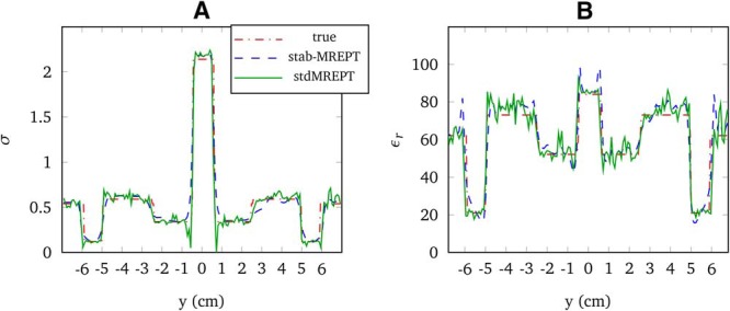
The variation of conductivity σ (A) and relative permittivity ϵr (B) along x = 0 for different methods.
In practical measurement, the data of are always polluted by noise at different levels. The noise tolerance of stabMREPT is tested using the simplified human brain model. The SNR is defined as , where is the simulated data. N is the added complex white Gaussian noise generated with a given noise level in decibel. is set to be 60 dB and in equation (5). The SG filter is used for calculating the derivatives of to smooth noisy data. Figure 12, A and B shows the results reconstructed by cr-MREPT. The accuracy of the results obtained is low. Results of stdMREPT are given in Figure 12, C and D. The results are severely degraded by the noise. Very large values and global oscillations are observed in the results. On the contrary, the noise has no strong effect on the results of σ reconstructed with stabMREPT, although the results for are slightly affected, as shown in Figure 12, E and F. Moreover, the reconstructed results are severely affected when the noise level is increased to be ≥50 dB. However, the effect of noise on stabMREPT becomes rapidly insignificant with an increase in SNR. Examples are given in Figure 12, G and H for stabMREPT with , a considerable improvement is observed. In contrast, performance of cr-MREPT and stdMREPT did not improve when SNR is increased from 60 to 65 dB. The effect of noise on stabMREPT is negligible when SNR is smaller than 70 dB.
Figure 12.

The noise tolerance of cr-MREPT (A and B), standard MREPT (stdMREPT) (C and D), and stabMREPT (E and F). The first and the second rows are reconstructed results of σ and ϵr, respectively. From left to right, the first 3 columns are reconstructed results of cr-MREPT, stdMREPT, and stabMREPT with 60 dB noise. The last row shows the results of stabMREPT with 65 dB noise (G and H). The Savitzky–Golay (SG) filter is used to calculate partial differentiations over for smoothing noisy data.
Discussion and Conclusion
Here, a viscosity-type regularization method is used to effectively improve the performance of the formerly proposed cr-MREPT, which is based on a first-order complex coefficient PDE. The proposed method is then named as stabMREPT. The regularization is implemented on the basis of the fact that adding the Laplacian term does not lead to a singularly disturbed problem. The PDE is discretized using FD method.
The reconstruction method based on the same PDE was named as cr-MREPT by Hafalir et al. (25). However, several drawbacks exist in this method, although it is rarely reported in the literature. Here, these drawbacks are analyzed in detail. Different numerical simulations are given for the purpose of illustration; 2 PDE properties are coupled. The governing equation of cr-MREPT is equation (1), which is in the form of pure convection–reaction PDE. It is well known in the literature that it is tricky to numerically solve this kind of PDE (40). With the complex coefficients, this kind of PDE has a smooth solution with some conditions, as discussed in Theory and Methodology. Therefore, directly using the convection–reaction PDE for reconstruction can be difficult.
The viscosity-type regularization method is then suggested. As illustrated in the paper, this method can efficiently mitigate the persistent artifacts existing in the convection–reaction PDE. The regularization parameter ρ needs to be positive and smaller than 1. It can be chosen as several times or a fraction of the maximum of , which is the x-component of . Blurring can be observed at the boundaries of different tissues, but the reconstruction accuracy can be considerably better. The accuracy of the proposed method is shown by numerical results obtained by using simple and complex phantoms. Good performances in several numerical experiments are observed by comparing them with other existing methods.
Although the noise tolerance is not yet good for practical use, it is already considerably better than stdMREPT and cr-MREPT. The noise tolerance of this method was compared with that of other methods. Another algorithm based on FEM will be implemented in the next step to add the regularization term only when it is needed. A regularization-based SG method (37) can be used for reconstructing from the measured noisy data, which will further reduce the influence of noise and increase the noise tolerance of the method.
Supplemental Materials
Footnotes
- MREPT
- Magnetic resonance electrical property tomography
- PDE
- partial differential equation
- MRI
- magnetic resonance imaging
- EPs
- electrical properties
- MR
- magnetic resonance
- LMT
- Local Maxwell Tomography
- cr-MREPT
- convection–reaction MREPT
- FD
- finite difference
- FEM
- finite element method
- stdMREPT
- standard MREPT
- stabMREPT
- stabilized MREPT
- SNR
- signal-to-noise ratio
- NRMSE
- normalized root-mean-square error
- SG
- Savitzky–Golay
- cr-MREPT
- convection–reaction MREPT
References
- 1. van der Kolk AG, Hendrikse J, Zwanenburg JJ, Visser F, Luijten PR. Clinical applications of 7T MRI in the brain. Eur J Radiol. 2013;82(5):708–718. [DOI] [PubMed] [Google Scholar]
- 2. Budinger TF, Bird MD, Frydman L, Long JR, Mareci TH, Rooney WD, Rosen B, Schenck JF, Schepkin VD, Sherry AD, Sodickson DK, Springer CS, Thulborn KR, U˘gurbil K, Wald LL. Toward 20T magnetic resonance for human brain studies: opportunities for discovery and neuroscience rationale. MAGMA. 2016;29(3):617–639. [DOI] [PMC free article] [PubMed] [Google Scholar]
- 3. Bulumulla SB, Lee S-K, Yeo TBD. Calculation of electrical properties from B1+ maps – a comparison of methods. Paper presented at: ISMRM 20th Annual Meeting and Exhibition; May 5–11, 2012; Melbourne, Australia http://cds.ismrm.org/protected/12MProceedings/files/3469.pdf [Google Scholar]
- 4. Gabriel C, Gabriel S, Corthout E. The dielectric properties of biological tissues: I. Literature survey. Phys Med Biol. 1996;41(11):2231–2249. [DOI] [PubMed] [Google Scholar]
- 5. Chaudhary SS, Mishra RK, Swarup A, Thomas JM. Dielectric properties of normal & malignant human breast tissues at radiowave & microwave frequencies. Indian J Biochem Biophys. 1984;21(1):76–79. [PubMed] [Google Scholar]
- 6. Surowiec AJ, Stuchly SS, Barr JB, Swarup A. Dielectric properties of breast carcinoma and the surrounding tissues. IEEE Trans Biomed Eng. 1988;35(4):257–263. [DOI] [PubMed] [Google Scholar]
- 7. Hall PS, Hao Y. Antennas and propagation for body centric communications. Paper presented at 2006 First European Conference on Antennas and Propagation; Nov 6-10, 2006, Nice, France http://ieeexplore.ieee.org/stamp/stamp.jsp?arnumber=4231209 [Google Scholar]
- 8. Crocetti S, Beyer C, Schade G, Egli M, Fröhlich J, Franco-Obregón A. Low intensity and frequency pulsed electromagnetic fields selectively impair breast cancer cell viability. PLoS ONE. 2013;11;8(9):e72944. [DOI] [PMC free article] [PubMed] [Google Scholar]
- 9. Stanley SA, Kelly L, Latcha KN, Schmidt SF, Yu X, Nectow AR, Sauer J, Dyke JP, Dordick JS, Friedman JM. Bidirectional electromagnetic control of the hypothalamus regulates feeding and metabolism. Nature. 2016;531(7596):647–650. [DOI] [PMC free article] [PubMed] [Google Scholar]
- 10. Vaughan T. RF (B1 & E) field, SAR and temperature for MRI: overview. Paper presented at: ISMRM scientific workshop 2014: Safety in MRI: guidelines, rationale and challenges; September 4-7, 2014; Washington DC http://cds.ismrm.org/protected/SafetyWorkshop14/Program/Syllabus/Vaughan.pdf [Google Scholar]
- 11. Jin JM, Chen J, Chew WC, Gan H, Magin RL, Dimbylow PJ. Computation of electromagnetic fields for high-frequency magnetic resonance imaging applications. Phys Med Biol. 1996;41(12):2719–2738. [DOI] [PubMed] [Google Scholar]
- 12. Haacke EM, Petropoulos LS, Nilges EW, Wu DH. Extraction of conductivity and permittivity using magnetic resonance imaging. Phys Med Biol. 1991;36(6):723. [Google Scholar]
- 13. Wen H. Noninvasive quantitative mapping of conductivity and dielectric distributions using RF wave propagation effects in high-field MRI. Paper presented at SPIE Conference; 2003. Accessed June 9, San Diego, CA: http://proceedings.spiedigitallibrary.org/proceeding.aspx?articleid=757767 [Google Scholar]
- 14. Katscher U, Voigt T, Findeklee C, Vernickel P, Nehrke K, Dössel O. Determination of electric conductivity and local SAR via B1 mapping. IEEE Trans Med Imaging. 2009;28(9):1365–1374. [DOI] [PubMed] [Google Scholar]
- 15. Voigt T, Katscher U, Doessel O. Quantitative conductivity and permittivity imaging of the human brain using electric properties tomography. Magn Reson Med. 2011;66(2):456–466. [DOI] [PubMed] [Google Scholar]
- 16. Katscher U, Kim DH, Seo JK. Recent progress and future challenges in MR electric properties tomography. Comput Math Methods Med. 2013;2013:546562. [DOI] [PMC free article] [PubMed] [Google Scholar]
- 17. van Lier AL, Raaijmakers A, Voigt T, Lagendijk JJ, Luijten PR, Katscher U, van den Berg CA. Electrical properties tomography in the human brain at 1.5, 3, and 7T: A comparison study. Magn Reson Med. 2014;71(1):354–363. [DOI] [PubMed] [Google Scholar]
- 18. Seo JK, Kim MO, Lee J, Choi N, Woo EJ, Kim HJ, Kwon OI, Kim DH. Error analysis of nonconstant admittivity for MR-based electric property imaging. IEEE Trans Med Imaging. 2012;31(2):430–437. [DOI] [PubMed] [Google Scholar]
- 19. Ammari H, Kwon H, Lee Y, Kang K, Seo JK. Magnetic resonance-based reconstruction method of conductivity and permittivity distributions at the Larmor frequency. Inverse Probl. 2015;31(10):105001–105024. [Google Scholar]
- 20. Sodickson DK, Alon L, Deniz CM, Brown R, Zhang B, Wiggins GC, Cho GY, Eliezer NB, Novikov DS, Lattanzi R, Duan Q, Sodickson LA, Zhu YS. Local Maxwell tomography with transmit-receive coil arrays for contact-free mapping of tissue electrical properties and determination of absolute RF phase. Paper presented at: The 20th Scientific Meeting of the International Society of Magnetic Resonance in Medicine (ISMRM '20); May 5–11, 2012; Melbourne, Australia http://cds.ismrm.org/protected/12MProceedings/files/0387.pdf [Google Scholar]
- 21. Sodickson DK, Alon L, Deniz CM, Ben-Eliezer N, Cloos M, Sodickson LA, Collins CM, Wiggins GC, Novikov DS. Generalized local Maxwell tomography for mapping of electrical property gradients and tensors. Paper presented at: 21st Scientific Meeting of the International Society of Magnetic Resonance in Medicine (ISMRM '21); April 20–26, 2013; Salt Lake City, UT http://cds.ismrm.org/protected/13MProceedings/files/4175.PDF [Google Scholar]
- 22. Song Y, Seo JK. Conductivity and permittivity image reconstruction at the Larmor frequency using MRI. SIAM J Appl Math. 2013;73:2262–2280. [Google Scholar]
- 23. Ibrahim TS, Lee R, Baertlein BA, Abduljalil AM, Zhu H, Robitaille PM. Effect of RF coil excitation on field inhomogeneity at ultra high fields: a field optimized TEM resonator. Magn Reson Imaging. 2001;19(10):1339–1347. [DOI] [PubMed] [Google Scholar]
- 24. Hayes CE, Edelstein WA, Schenck JF, Mueller OM, Eash M. An efficient, highly homogeneous radio frequency coil for whole-body NMR imaging at 1.5T. J Magn Reson. 1985;63(3):622–628. [Google Scholar]
- 25. Hafalir FS, Oran OF, Gurler N, Ider YZ. Convection-reaction equation based magnetic resonance electrical properties tomography (cr-MREPT). IEEE Trans Med Imaging. 2014;33(3):777–793. [DOI] [PubMed] [Google Scholar]
- 26. Codina R. Comparison of some finite element methods for solving the diffusion-convection-reaction equation. Comput Methods Appl Mech Eng. 1998;156(1–4):185–210. [Google Scholar]
- 27. Huang SY, Hou L, Wu J. MRI-based electrical property retrieval by applying the finite-element method (FEM). IEEE Trans Microw Theory Tech. 2015;63(8):2482–2490. [Google Scholar]
- 28. Ammari H, Grasland-Mongrain P, Millien P, Seppecher L, Seo JK. A mathematical and numerical framework for ultrasonically-induced Lorentz force electrical impedance tomography. J Math Pures Appl. 2015;103(6):1390–1409. [Google Scholar]
- 29. Roos HG, Stynes M, Tobiska L. Robust Numerical Methods for Singularly Perturbed Differential Equations. Springer-Verlag, Berlin Heidelberg; 2008. Berlin, Heidelberg, Germany. [Google Scholar]
- 30. Cervera M, Chiumenti M, Codina R. Mixed stabilized finite element methods in nonlinear solid mechanics: Part I: Formulation. Comput Methods Appl Mech Eng. 2010;199:2559–2570. [Google Scholar]
- 31. Lomax H, Pulliam TH, Zingg DW. Fundamentals of Computational Fluid Dynamics. Springer-Verlag, Berlin Heidelberg; 2001. Berlin, Heidelberg, Germany. [Google Scholar]
- 32. von Kowalevsky S. Zur theorie der partiellen differentialgleichung. J Reine Angew Math. 1875;80:1–32. [Google Scholar]
- 33. Hannani SK, Stanislas M, Dupont P. Incompressible Navier–Stokes computations with SUPG and GLS formulations—a comparison study. Comput Methods Appl Mech Eng. 1995;124(1–2):153–170. [Google Scholar]
- 34. Savitzky A, Golay MJE. Smoothing and differentiation of data by simplified least squares procedures. Anal Chem. 1964;36:1627–1639. [Google Scholar]
- 35. COMSOL [computer program]. Version 5.0 Burlington, Vermont: COMSOL, Inc.; 2015. [Google Scholar]
- 36. Gurler N, Ider Y. FEM based design and simulation tool for MRI birdcage coils including eigenfrequency analysis. Paper presented at: 8th Annual Conference on Multiphysics Simulation and its Applications, 2012 Milan, Italy https://www.comsol.asia/paper/fem-based-design-and-simulation-tool-for-mri-birdcage-coils-including-eigenfrequ-13408s [Google Scholar]
- 37. Toonkum P, Suwanwela NC, Chinrungrueng C. Reconstruction of 3D ultrasound images based on cyclic regularized Savitzky-Golay filters. Ultrasonics. 2011;51(2):136–147. [DOI] [PubMed] [Google Scholar]
- 38. Paige CC, Saunders MA. LSQR: An algorithm for sparse linear equations and sparse least squares. ACM Trans Math Softw. 1982;8(1):43–71. [Google Scholar]
- 39. Gabriel C. Compilation of the dielectric properties of body tissues at RF and microwave frequencies. Technical Report N.AL/OE-TR-1996-0037; Occupational and Environmental Health Directorate; Radiofrequency Radiation Division; Brooks Air Force Base, TX; June 1996. [Google Scholar]
- 40. Hauke G. A simple subgrid scale stabilized method for the advection-diffusion-reaction equation. Comput Methods Appl Mech Eng. 2002;191(2728):2925–2947. [Google Scholar]
- 41. Yarnykh VL. Actual flip-angle imaging in the pulsed steady state: A method for rapid three-dimensional mapping of the transmitted radiofrequency field. Magn Reson Med. 2007;57(1):192–200. [DOI] [PubMed] [Google Scholar]
- 42. Chung S, Kim D, Breton E, Axel L. Rapid B1+ mapping using a preconditioning RF pulse with TurboFLASH readout. Magn Reson Med. 2010;64(2):439–446. [DOI] [PMC free article] [PubMed] [Google Scholar]
- 43. Morrell GR, Schabel MC. An analysis of the accuracy of magnetic resonance flip angle measurement methods. Phys Med Biol. 2010;21;55(20):6157–6174. [DOI] [PubMed] [Google Scholar]
Associated Data
This section collects any data citations, data availability statements, or supplementary materials included in this article.