Renewing Felsenstein’s Phylogenetic Bootstrap in the Era of Big Data

Abstract

Felsenstein’s article describing the application of the bootstrap to evolutionary trees is one of the most cited papers of all time. The bootstrap method, based on resampling and replications, is used extensively to assess the robustness of phylogenetic inferences. However, increasing numbers of sequences are now available for a wide variety of species, and phylogenies with hundreds or thousands of taxa are becoming routine. In that framework, Felsenstein’s bootstrap tends to yield very low supports, especially on deep branches. We propose a new version of phylogenetic bootstrap, in which the presence of inferred branches in replications is measured using a gradual “transfer” distance, as opposed to the original version using a binary presence/absence index. The resulting supports are higher, while not inducing falsely supported branches. Our method is applied to large mammal, HIV, and simulated datasets, for which it reveals the phylogenetic signal, while Felsenstein’s bootstrap fails to do so.

The bootstrap is a widely used statistical method to study the robustness, bias and variability of numerical estimates^1,2. It involves resampling with replacement from the original dataset to obtain replications of the original estimate, and then typically to compute the variance and distribution of this estimate. In 1985, Joseph Felsenstein proposed the application of the bootstrap to assess the robustness (or repeatability) of phylogenetic trees³. Given a sequence alignment and a reference tree inferred on it, the procedure is: (i) resample, with replacement, the sites of the alignment to obtain pseudo-alignments of the same length, (ii) infer pseudo-trees using the same inference method, and (iii) measure the support of every branch in the reference tree as the proportion of pseudo-trees containing that branch. The usefulness, simplicity and interpretability of this method made it extremely popular in evolutionary studies, to the point that it is generally required for publication of tree estimates in a wide variety of domains (molecular biology, genomics, systematics, ecology, epidemiology, etc.). Felsenstein’s article has been cited more than 32,000 times and is ranked in the top 100 of the most cited scientific papers of all time⁴. However, the use of Felsenstein’s bootstrap was questioned on biological grounds, notably regarding the assumptions of site independence and homogeneity⁵. Moreover, the statistical meaning of Felsenstein’s bootstrap proportions (FBPs) has been the subject of intense debate⁶, the main questions being whether FBPs can be seen as the confidence levels of some test, and whether or not they are biased^7–10. Several methods^{9, 11–12} have been proposed to correct FBP to better agree with standard ideas of confidence levels and hypothesis testing. These works greatly contributed to the understanding of what Felsenstein’s bootstrap is and what it is not. However, FBP correction methods are limited to relatively small data sets for mathematical and computational reasons (e.g. double bootstrapping), and the original method is still highly used (~2,000 citations in 2016). As stated by Soltis et al.¹³: “consensus has been reached among practitioners, if not among statisticians and theoreticians”, and “many systematists have adopted Hillis and Bull’s “70%” value⁷ as an indication of support”. The alternatives to FBPs are the Bayesian posterior probabilities of the tree branches¹⁴, which are difficult to obtain with large datasets for computational reasons, and the approximate branch supports^15–16, which are fast but provide only a local view. The bootstrap is also computationally heavy, but is easily parallelized and fast algorithms have been designed^17–18.

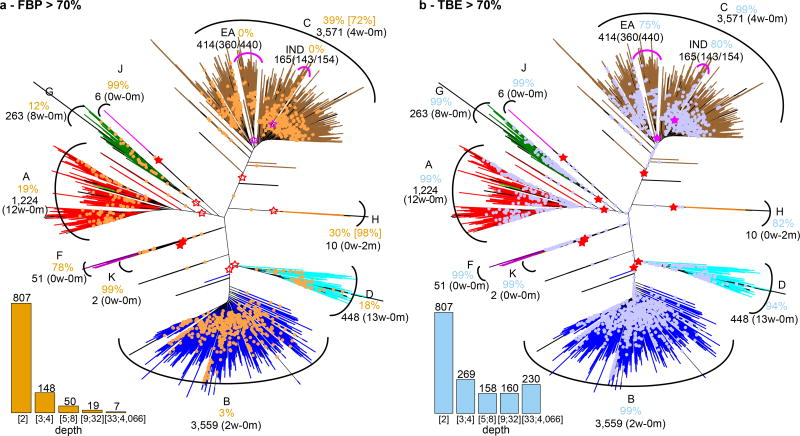
It is commonly acknowledged¹³ that Felsenstein’s bootstrap is not appropriate for large datasets containing hundreds or thousands of taxonomic units (taxa), which are now common thanks to high-throughput sequencing technologies. While such datasets generally contain a lot of phylogenetic information, the bootstrap proportions tend to be low, especially when the tree is inferred from a single gene, or only a few genes, as illustrated in Fig. 1a with a dataset of ~9,000 HIV-1 group M DNA polymerase (pol) sequences. The strongest signal in such a phylogeny generally corresponds to the deep branching of the subtypes. This signal is immediately visible here, and in agreement with the common belief about subtype branching¹⁹, but some of the subtypes are not supported (A, B, D, G) and their branching is not supported either (e.g. the grouping of C and H). When using a medium-sized dataset of ~550 randomly selected sequences, the FBPs are higher, with most subtypes supported at 70% or more. However, their deep branching is still unresolved (Fig. ED5).

Fig. 1. Felsenstein (FBP) and transfer (TBE) bootstrap supports on the same tree with 9,147 HIV-1M pol sequences.

(a): FBP; (b): TBE. Subtypes are colorized; recombinant sequences are black; dots correspond to branches with support >70%⁷. Supports are given for the tree clades that are closer to the subtypes (red stars, filled when support >70%); for each of these clades we provide, using jpHMM predictions, the number of wrong (w) taxa that do not belong to the corresponding subtype, and the number of missing (m) taxa that belong to the subtype but not to the clade. For the C and the H, these clades are not supported by FBP, but there exist neighbouring clades with FBP >70%, and these are shown in brackets. The same approach is applied to the C sub-epidemics in India (IND) and Eastern Africa (EA); the ratio provides the coverage of the clade, i.e. the number of studied (e.g. Indian) taxa in the clade versus the total number of those taxa in the dataset. The South American clade (SA, not shown, included in EA) is supported by TBE but not by FBP (73% vs. 14%, 15 taxa, 14/14). The histograms provide the number of branches with support >70% depending on branch depth, which is measured by the number of taxa in the smaller of the two clades defined by the given branch.

The reason for such degradation is explained by the core methodology of Felsenstein’s bootstrap. A replicated branch must match a reference branch exactly to be accounted for in the FBP value. A difference of just one taxon (highly likely with large datasets) is sufficient for the replicated branch to be counted absent while it is nearly identical to the reference branch^13,20. There are many biological and computational reasons for the existence of “rogue” taxa with unstable phylogenetic positions: convergence, recombination, sequence and tree errors, etc. The standard approach^20–24 is to remove these taxa and relaunch the analysis, but this is statistically questionable and computationally expensive. Moreover, with a large number of taxa and a low number of sites, the phylogenetic signal is weak. Then, the inferred branches are likely to have errors and a large fraction of taxa may be unstable, even in the absence of model misspecification of any sort, and without long branches.

A statistical approach

Our approach has a simple but sound statistical basis, partly inspired by Sanderson’s monophyly index²⁵ and our work on gene clusters obtained from expression data²⁶ (both are tailored for rooted trees). We replace the branch presence proportion (i.e. the expectation of a {0,1} indicator function) of Felsenstein’s bootstrap, by the expectation of a refined, gradual function in the [0,1] range, quantifying the branch presence in the bootstrap trees. In doing so, we admit that the inferred branch is not simply correct or incorrect (as with FBP), but that it may contain some errors. Our ultimate aim is to quantify these errors and the presence of the inferred branch in the true tree, using the plug-in principle (see below). We use the “transfer” distance^27–29, where the distance δ(b,b*) between a branch b of the reference tree T and a branch b* of a bootstrap tree T* is equal to the number of taxa that must be transferred (or removed), in order to make both branches identical (i.e. both split identically the set of taxa). To measure the presence of b in T*, we search the branch in T* that is closest to b and use the “transfer index” ϕ(b,T*) = Min_b*∈T*{δ(b,b*)}. This index has several important and useful properties. Let l be the number of taxa. Any branch b splits the taxa into two subsets; let p be the size of the smaller subset induced by b. We have (Methods):

• ϕ(b,T*) = 0 if and only if b belongs to T*;

• ϕ(b,T*) ≤ p − 1;

• ϕ(b,T*)/(p − 1) is very close to 1 when T* is random and l is large (say >100);

• ϕ(b,T*) is computed recursively in time proportional to l, just as FBP.

Based on these properties, we define the transfer bootstrap expectation (TBE) as:

$$\text{TBE}(b)=1-\frac{\overline{\mathrm{\varphi }(b,T^{\ast })}}{p-1},$$

where the numerator is the average transfer index among all bootstrap trees. It is easily seen that TBE ranges from 0 to 1, where 0 means that the bootstrap trees are random regarding b, and 1 means that b appears in all bootstrap trees. Moreover, considering the same set of bootstrap trees, TBE(b) is necessarily larger than FBP(b) and the difference is substantial for deep branches, while TBE(b) = FBP(b) when b defines a (shallow) “cherry” (i.e. p = 2). Importantly, we shall see that TBE supports very few branches showing substantial contradictions with the true tree, when used with common thresholds, typically 70%⁷ or higher (Fig. 2c–d, ED2–ED3, ED7–ED8).

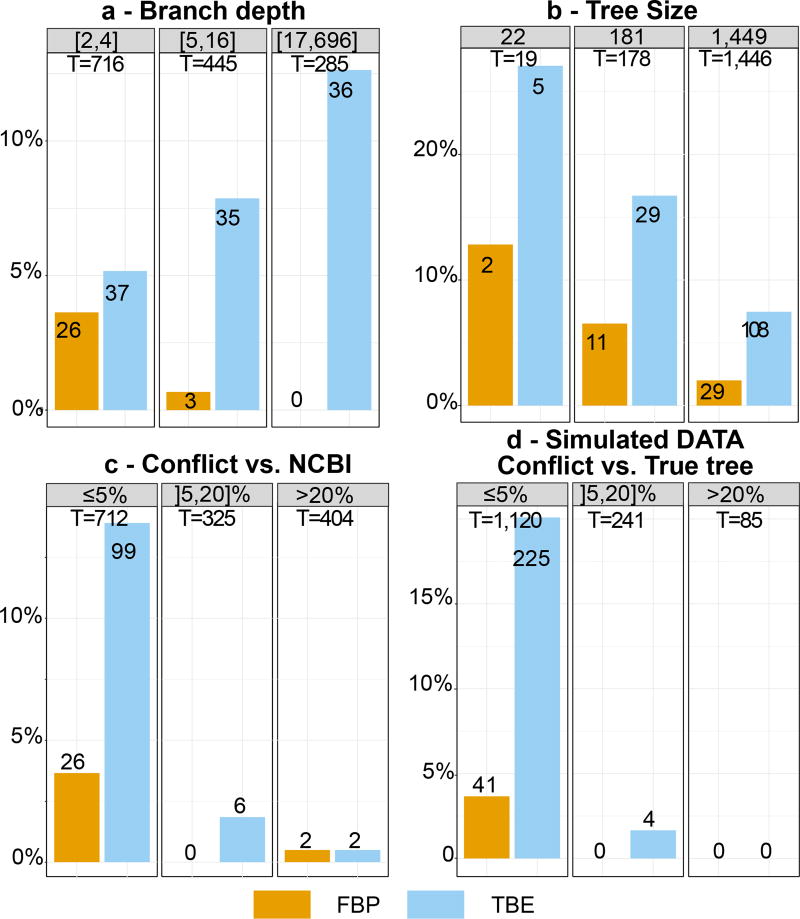
Fig. 2. Felsenstein (FBP) and transfer (TBE) bootstrap supports with 1,449 COI-5P mammal sequences – FastTree phylogeny.

Graphs (a) to (d) refer to branches with supports >70%⁷, with the vertical axis denoting the percentage of these branches in a given condition (e.g. (b): 19 internal branches with 22-taxon trees, and 2/19 ≈ 10% of branches with FBP >70%). (a) Supports regarding branch depth (see note to Fig. 1). (b) Supports regarding tree size (i.e. number of taxa). (c) Supports regarding percentage of quartet conflicts with NCBI taxonomy (≤5%: low conflict level;] 5,20]% moderate; ≥20%: high). (d) Same as (c) but regarding the true tree used for simulations.

All these properties are highly desirable: easy computation, higher supports than FBP, low number of falsely supported branches. Moreover, TBE has a simple and natural interpretation; for instance, with l = 1, 000 and p = 200, TBE(b) = 95% means that, on average, (200 − 1) × 0.05 ≈ 10 taxa have to be transferred to recover b in bootstrap replicate trees. Moreover, we can define an instability score for each taxon, based on the number of times it is transferred in TBE computations. This interpretation is radically different from that of FBP, where b is assessed globally as correct or erroneous. With TBE, nearly correct branches will also be likely supported.

TBE uses the same resampling with replacement procedure as FBP, and thus inherits some of its statistical properties^3,6,9, as well as usual properties of the bootstrap method^1,2. Notably, TBE relies on the same assumptions as FBP regarding site independence and homogeneity, but these assumptions can be relaxed⁶, for instance using block bootstrapping³⁰. Just like FBP³, TBE(b) cannot be interpreted as the probability for the branch b to belong to the true phylogeny. While deep mathematical approaches^6,9–12,31 have been proposed to connect FBP to hypothesis-testing theory, TBE should not be interpreted as the confidence level of some statistical test (with null and alternative hypotheses, distribution of test statistics under the null, etc.). TBE is better and more simply interpreted in terms of repeatability: TBE(b) estimates the extent by which branches identical or similar to b would be recovered when applying the same tree inference method to a new sample of the same size drawn from the same site distribution as the original sample. With large samples, the empirical distribution obtained from observed data comes close to the (unknown) underlying distribution of this data, and sampling with replacement in the empirical distribution is asymptotically equivalent to drawing samples from the underlying distribution^1,2. The convergence rate is unknown with models as complex as the ones used in phylogenetics, but our simulation results show that moderate sample sizes suffice to obtain good approximations (Fig. ED10). When the sample size is extremely large, as in phylogenomic studies using genome-scale sequence alignments³², both FBP and TBE are expected to be nearly equal to 1 for all branches. Again, this should not be interpreted in terms of absolute truth regarding the phylogenetic inferences, but it simply reflects the closeness of the empirical and underlying distributions and the very small variability of tree estimates. In fact, a high level of repeatability is necessary to trust phylogenetic inferences, but it may be not sufficient. As quoted by Felsenstein³, the bootstrap “may be misleading if the method used to infer phylogenies is inconsistent”. This applies both to FBP and TBE, and typically to inference methods subject to long-branch attraction. With a consistent, unbiased inference method, we expect the plug-in principle1^1,2,6,9 to apply, stating that the distribution of the distance between the true tree and the inferred tree can be well-approximated by the distribution of the distance between the inferred and bootstrap trees. Using both real and simulated data, we shall see that this principle does apply with maximum likelihood estimation, a typically consistent phylogenetic inference method³³. In this setting, TBE informs us regarding the (transfer, quartet-based) distance between the inferred branch and the true tree, and rarely supports poor branches. Moreover, the ability of TBE to identify rogue taxa makes it possible to study them further, understand why they are phylogenetically unstable, and revise the branch supports.

Analysis of mammal data

We first studied the advantage of TBE on a large phylogeny of 1,449 mammals, obtained from a usual barcoding marker (COI-5P). The reference and bootstrap trees were inferred by maximum likelihood from the protein alignment (527 sites) using both FastTree³⁴ and RAxML with rapid bootstrap¹⁷ to check that similar conclusions were drawn with different inference methods. To study the impact of the number of taxa, we randomly selected small (22 taxa) and medium (181 taxa) datasets and performed the same analyses. The results were compared to the NCBI taxonomy³⁵, which represents current thinking about mammals’ evolutionary history. To cope with the low resolution of the NCBI taxonomy, we used a quartet-based topological distance, rather than the transfer distance. For all inferred branches, we measured the quartet-based percentage of conflicts with the NCBI taxonomy, and the same approach was used to assess the topological accuracy of FastTree and RAxML phylogenies. As expected in this type of study based on a unique marker, the inferred topologies were relatively poor, and thus challenging for branch support methods. However, RAxML was more accurate than FastTree, with higher branch supports, as generally observed with rapid bootstrap¹⁶ (Fig. ED2–ED3).

Results (Fig. 2a–c, ED2–ED3) indicate clearly that TBE provides some support for deep branches, while FBP does not. As expected, the supports of shallow branches are similar, and the impact of TBE is more pronounced with a large number of taxa, but still of interest with medium-sized datasets. Comparisons with the NCBI taxonomy show that TBE supports a larger number of weakly contradicted branches than FBP, which fulfils one of its objectives (nearly correct branches must be supported), while the number of supported branches with moderate to high quartet conflicts remains very low. These results are confirmed by simulations (Fig. 2d, ED7–ED8).

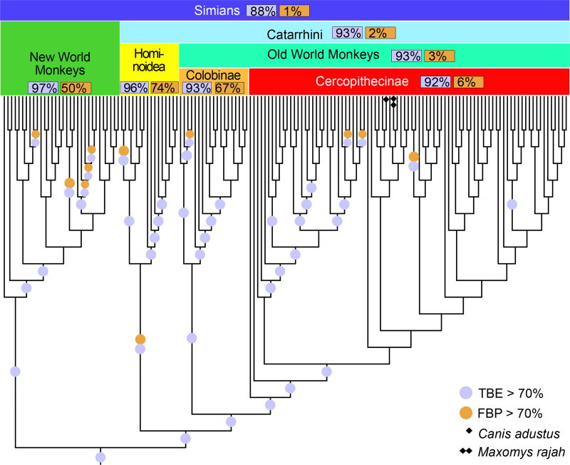
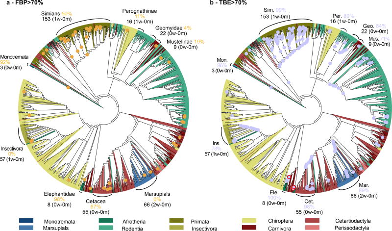
The advantage of TBE appears clearly when inspecting the tree clades. For example (Fig. 3), the simian clade inferred by FastTree has a strong support with TBE, while FBP is nearly null due to a high number of rogue taxa in the bootstrap trees, and the same holds true for several sub-clades. This clade includes all simian sequences (152), plus two non-simian taxa: Maxomys rajah and Canis adustus. The latter is not a rogue taxon: its sequence is incomplete and very close to the simian sequences for the part being available, and its position is very stable in the bootstrap trees. In contrast, Maxomys rajah is a rogue taxon, and is detected as such by TBE (659/1000 transfers when computing the support of the simian clade). Similar results were found with other well-established clades and using RAxML (Fig. 4). Both FBP and TBE support some small clades, namely the monotremes and elephantidae. However, FBP does not support any deep branches, except cetaceans (67%), and to some extent, simians (50%). TBE provides strong supports for these two groups, but also for five other groups, such as marsupials and insectivores. The latter clade (FBP: 0%, TBE: 78%) contains all insectivores of the NCBI taxonomy, plus one extra taxon (Plecotus cf. strelkovi), which again is detected by TBE as a rogue taxon (965/1000 transfers). In comparison, the removal of rogue taxa²⁴ does not significantly improve FBP (8 and 3 taxa are removed with FastTree and RAxML, respectively, but the number of branches with FBP >70% remains the same). This is explained by hundreds of taxa, which are relatively unstable, but not removed.

Fig. 3. Felsenstein (FBP) and transfer (TBE) bootstrap supports – FastTree phylogeny using 1,449 COI-5P mammal sequences – Focus on the simian clade.

All simian sequences are included, but two additional non-simian sequences are added, one rogue taxon (Maxomys rajah, detected by TBE, see text) and one stable but erroneous taxon with partial sequence (Canis adustus); this simian tree is very close to the NCBI taxonomy (<2.5% of contradicted quartets, when both erroneous taxa are pruned).

Fig. 4. Felsenstein (FBP) and transfer (TBE) supports on the same tree with 1,449 COI-5P mammal sequences – RAxML with rapid bootstrap.

(a): FBP; (b): TBE. This phylogeny is more accurate than the one by FastTree (27% versus 38% of contradicted quartets, respectively), but still relatively poor, especially regarding deep nodes and larger groups. For example, rodents and chiropters are not monophyletic and are distributed in several subtrees. However, some parts of the tree are more accurate. A few clades are highlighted, corresponding (almost) exactly to the NCBI taxonomy. For example, all elephantidae taxa are recovered by RAxML in a single clade, containing elephantidae only, while insectivores are included in a clade containing one extra taxon. To select these clades, we minimized the transfer distance with the NCBI taxonomy, in case of ambiguity. See note to Fig. 1 and Methods for details.

Analysis of HIV data

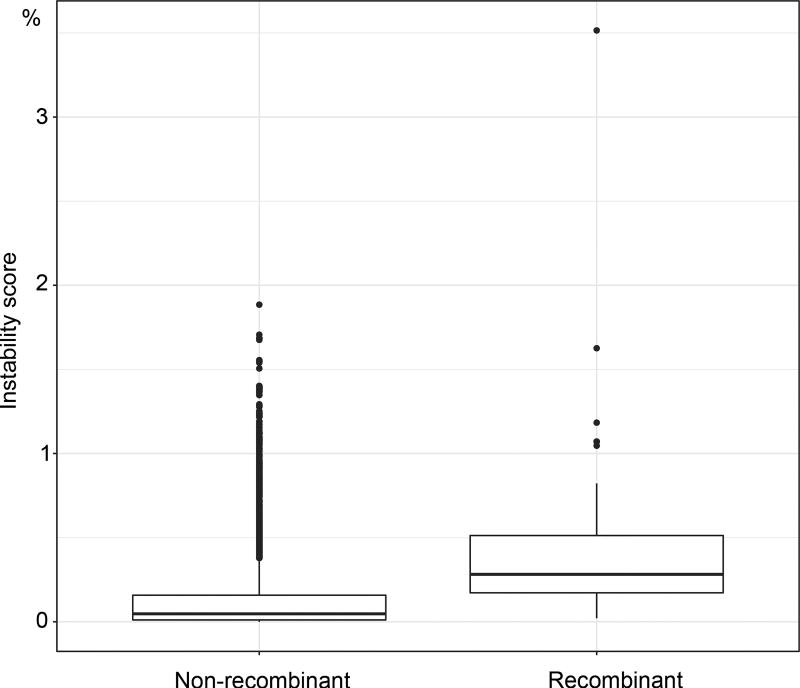
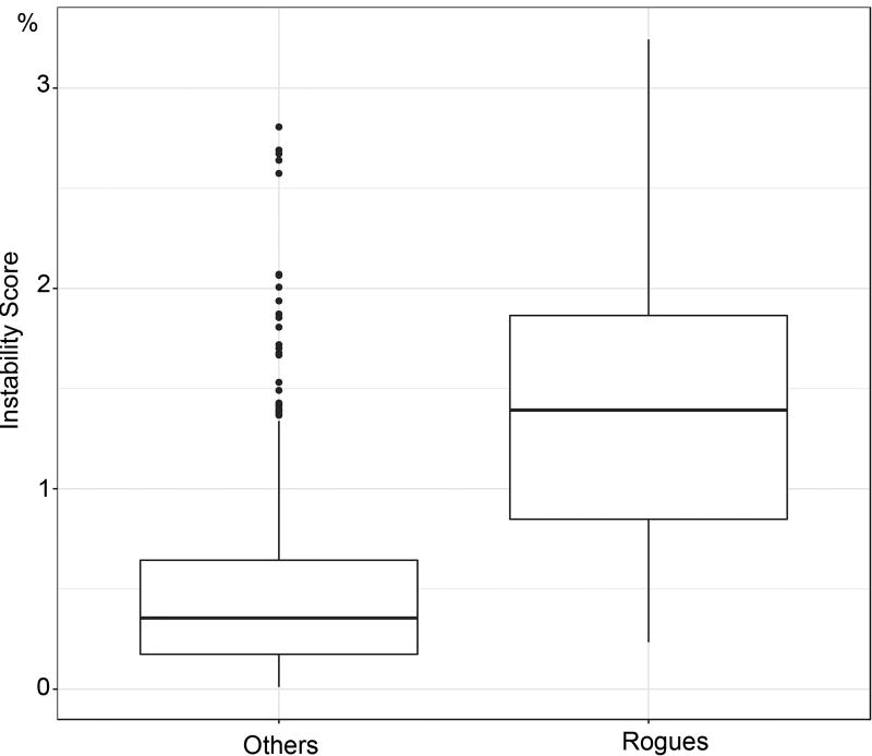
We applied our method to a large dataset of 9,147 HIV-1 group M pol sequences. Such large datasets are increasingly common in molecular epidemiology and phylodynamics³⁶. We only retained sequences annotated as non-recombinant by the Los Alamos HIV-1 DB using a fast filtering approach. Among these, 48 recombinant sequences were still detected by jpHMM³⁷. These 48 sequences were kept in the analyses to study the impact of recombinant sequences, as their presence is inevitable in any HIV dataset. In contrast to mammals, the tree topology of HIV-1M strains is essentially unknown. Moreover, it is intrinsically unstable as reconstructing a tree with so many relatively short and possibly recombinant sequences is a very hard task. Thus, the main expectation is to observe a clear separation between the subtypes. We built the reference and bootstrap trees using FastTree on the DNA sequence alignment (1,043 sites), and performed the same analyses using smaller subsets of 35 and 571 sequences. While the deep branching of the subtypes¹⁹ is poorly supported by FBP (Fig. 1a), it becomes apparent with TBE, where all subtypes have a support larger than 80%, and close to 100% in most cases (Fig. 1b, ED5). For example, the subtype B clade (3,559 taxa) has FBP = 3% and TBE = 99%. This clade contains all subtype B sequences, plus 2 taxa detected as recombinant by jpHMM, meaning that both supports are likely right in saying that this clade is incorrect (FBP), and nearly correct (TBE), but FBP fails to detect any phylogenetic signal, whereas it is quite strong here. The same holds true with other well described clades. For example, TBE supports the identification of regional variants of HIV-1 subtypes that are of epidemiological importance: the East-African, Indian, and South American subtype C variants, which FBP fails to support. TBE provides a substantial support to a much larger number of deep branches. Again, the advantage in using TBE is higher with large data sets (Fig. ED4), but still apparent with 571-taxon datasets, where the deep subtype branching and C sub-epidemics are supported by TBE but not FBP (Fig. ED5). An important feature of TBE is that the supports may be non-local, but attached to “caterpillar-like” paths (Fig. 1b, e.g. subtype C). With HIV-1M data, this corresponds to the fact that the subtype roots are usually not well defined due to recombinant and ancient sequences. Moreover, the instability score among recombinant sequences is clearly higher than in the sequences not detected as recombinant (Fig. ED6), supporting the biological soundness of the approach and its power in detecting recombination and rogue taxa.

Analysis of simulated data

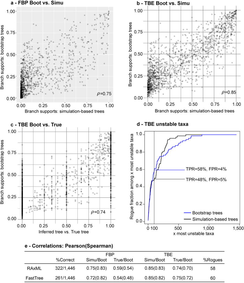
To check that TBE does not support erroneous branches, we performed extensive computer simulations with various tree sizes and phylogenetic signal levels. We also added unstable taxa having weaker phylogenetic signal than the others. The results are highly similar to those with real data regarding the support of deep branches and the tree size (Fig. ED7–ED8). In all the conditions we examined, TBE supported very few branches showing substantial contradictions with the true tree, and the rogue taxa exhibited lower stability (Fig. ED9). In the absence of rogue taxa (Fig. ED7), the gain of TBE was still substantial compared to FBP, with almost twice as many branches with support >70%, thus showing the importance of accounting for the global instability of the inferred tree. Moreover, we checked the interpretation of TBE as a measure of repeatability (Fig. ED10) by comparing TBE to its counterpart computed from simulated alignments, rather than bootstrap pseudo-alignments; both simulation- and bootstrap-based supports are highly correlated (0.85) with alignments of moderate length (~500) and have analogous performance in detecting rogue taxa. Lastly, we checked the validity of the plug-in principle by comparing TBE to the normalised transfer index measuring the similarity between the inferred branch and the true tree (Fig. ED10). Again a high correlation (0.74) was found. When performing the same experiments with FBP, similar or slightly lower correlations were observed, likely due to the discontinuous nature of FBP.

Discussion

The transfer bootstrap thus provides a measure of branch repeatability (or robustness). The results clearly demonstrate its usefulness, especially with deep branches and large datasets, where branches known to be essentially correct are supported by TBE but not by FBP. Moreover, when combined with (consistent) maximum-likelihood tree estimation, TBE rarely supports poor branches. Importantly, TBE supports are easily interpreted as fractions of unstable taxa. Although our results suggest that 70% is a reasonable threshold to start with (Fig. ED2, ED3, ED4, and ED8), we do suggest that it is better for users to interpret the TBE values depending on the data and the phylogenetic question being addressed (e.g. lower TBE support threshold with HIV and possibly recombinant sequences, than with mammals). Moreover, our experiments demonstrate the ability of the transfer index to detect unstable taxa responsible for low supports. Lastly, the approach is applicable to rapid bootstrap^17–18 (Fig. 4, ED3) and could be extended to parametric bootstrap² and Bayesian branch supports¹⁴.

Methods

Transfer distance and index: definitions and properties

The transfer distance²⁷, also called R-distance²⁸, was introduced to compare partitions in cluster analysis. In this context, the transfer distance is equal to the minimum number of elements to be transferred (or removed) to transform one partition into the other. Tree branches are commonly seen as bipartitions or splits, as a branch divides the taxa into two subsets situated on its two sides. The most used topological distance between two trees is the Robinson and Foulds distance³⁸, which is equal to the number of bipartitions that belong to one tree but not the other. As quoted by Lin et al.²⁹, the bipartition distance is overly sensitive to some small tree changes, possibly involving a unique taxon. Those authors proposed using the transfer distance and designed algorithms to compute a more robust “matching” distance between trees, a different task, but related to the aim of this article. In the following, we first provide basic definitions (see Semple and Steel³⁹ for a text book on phylogenetic trees), and then demonstrate the properties of the transfer distance in a bootstrap context.

Let X be a fixed set of l taxa. An X-tree is a phylogenetic tree with l leaves labelled by the taxa of X. All (reference, bootstrap) trees discussed here are X-trees, meaning that they are labelled by the same set of l taxa. Any branch of an X-tree defines a bipartition of X, and the topology of an X-tree can be recovered from its bipartition set. Thus, we will use both terms (branch, bipartition) indifferently, depending of the context. Any bipartition b of X can be encoded by a {0,1} vector v(b) of length l, where the taxa on the same side of the bipartition are encoded by the same value. Note that b is also encoded by $\overline{\mathbf{\text{v}}}(\mathit{\text{b}})$ the negation of v(b) (i.e. the 0s are turned into 1s and vice versa). Moreover, the smaller of the two subsets induced by a bipartition b will be called here the “light side” of b, and p will denote the size of the light side of b (p ≤ l − p). One says that a bipartition is “trivial” when it has a unique taxon in its light side (p = 1). An X-tree defines l trivial bipartitions corresponding to each of the taxa. These trivial bipartitions are contained in every X-tree, while the other non-trivial bipartitions define the core of the tree topology and are the central subject of phylogenetic studies.

The transfer distance δ(b,b*) between a bipartition b of the reference tree T and a bipartition b* of a bootstrap tree T* is equal to the number of taxa that must be transferred (or removed) to make both bipartitions identical. The transfer distance is easily defined and computed using the Hamming distance H between v(b) and v(b*):

$$\mathrm{\delta }(b,b^{\ast })=\mathit{\text{Min}}\{H(\mathbf{v}(b),\mathbf{v}(b^{\ast })),H(\overline{\mathbf{v}}(b),\mathbf{v}(b^{\ast }))\}$$

To measure the presence of b in T*, we search the bipartition in T* that is closest to b and use the transfer index ϕ(b,T*) = Min_b*∈T*{δ(b,b*)}. Based on above definitions, δ(b,b*) = 0 if and only if v(b) and v(b*) define the same bipartition of X. Thus, the transfer index satisfies:

$$\mathrm{\varphi }(b,T^{\ast })=0\text{ if and only if }b\in T^{\ast }.$$

Moreover, let b be any given bipartition of T and t be a taxon in the light side of b. The trivial bipartition b* = {t}/X − {t} is found in any bootstrap tree T* and δ(b,b*) = p − 1. There may well be another bipartition closer to b in T*, but at least this ensures that:

$$\mathrm{\varphi }(b,T^{\ast })\le p-1,$$

and thus, the transfer support TS satisfies:

$$\mathit{\text{TS}}(b,T^{\ast })=1-\frac{\mathrm{\varphi }(b,T^{\ast })}{p-1}\in [0,1]\text{ and}$$

$$\mathit{\text{TS}}(b,T^{\ast })=1\text{ if and only if }b\in T^{\ast }.$$

Let 1_b(T*) be the indicator function equal to 1 when b ∈ T* and 0 otherwise. For any bipartition b and tree T*, we have 1_b(T*) ≤ TS(b,T*). The Felsenstein bootstrap proportion (FBP) is equal to the average of 1_b(T*) over the set of bootstrap trees, while the transfer bootstrap expectation (TBE) is equal to the average of TS(b,T*). Thus, when using the same set of bootstrap trees, we necessarily have FBP(b) ≤ TBE(b). When b is a “cherry” (p = 2), we have 1_b(T*) = TS(b,T*) and thus FBP(b) = TBE(b). With deeper bipartitions, we generally observe that in the presence of a significant phylogenetic signal, only a small number of taxa need to be transferred to make b identical to a bipartition in T*, while the strict presence of b in T* can be relatively rare; the difference between FBP(b) and TBE(b) can then be substantial.

The transfer distance and index are related to parsimony. The branch b is equivalent to a binary {0,1} character; assuming that the tips of T* are labelled accordingly, we can define PA(b,T*), which is the minimum number of changes along T* branches required to explain the tips labels. When b belongs to T*, we have PA(b,T*) = 1, and the more shuffled the 0s and 1s among the tips of T*, the higher is PA(b,T*). It is easy to see that PA(b,T*) ≤ ϕ(b,T*)+1. Indeed, let b* be a branch in T* such that ϕ(b,T*) = δ(b,b*) and assume, without loss of generality, that δ(b,b*) is equal to the number of tips labelled 1 in the light side of b* plus the number of tips labelled 0 in the heavy side of b* (in other words, the light side of b* is mostly 0 and the heavy side is mostly 1). Now consider that all internal nodes in the light side are 0 and all internal nodes in the heavy side are 1; this implies a number of changes equal to ϕ(b,T*)+1, which by the definition of parsimony is larger than or equal to PA(b,T*). Parsimony is thus another option to measure branch presence, but it is inappropriate in our context. For example, consider a reference branch b = AB|CD, where A, B, C and D are four large “corner” subtrees, and a tree T* with an internal branch b* grouping the corner subtrees the other way around (e.g. b* = AC|BD, meaning that A and C sit on one side of b*, and B and D on the other side). Then, PA(b,T*) is equal to 2, a very low value, while T* is phylogenetically very different from b since both clades defined by b are mixed. In that case, the transfer index between b and T* is much larger and equal to the minimum size of A, B, C and D.

Recursive computation of the transfer index

Lin et al.²⁹ describe a recursive algorithm to compute all transfer distances between any given bipartition b of T and all bipartitions of another tree T’ (see also Bréhélin et al.²⁶). This algorithm is easily transformed to compute the transfer index. The principle is as follows:

1. Map all the leaves of the light side of b to 0, the others to 1, and apply the same mapping to the leaves of T*. Moreover, root T* at any internal node.

2. With a single postorder tree traversal, one can compute the number of leaves labelled 0 and the number of leaves labelled 1 for every subtree in T*.

3. Let l₀ be the number of leaves labelled 0 and l₁ be the number of leaves labelled 1 in the subtree attached below a given bipartition b*. The transfer distance between b and b* is given by (think to the missing 0s and the 1s to be removed in b* subtree, and vice versa):

   $$\mathrm{\delta }(b,b^{\ast })=\mathit{\text{Min }}\{p-l_0+l_1,l-p-l_1+l_0\}.$$

   This distance can be computed during the postorder traversal as well as the transfer index ϕ(b,T*), which is the minimum of δ(b,b*) for all bipartitions of T*.

This algorithm has linear time complexity, and thus computing TBE for all bipartitions in T with r bootstrap replicates has a time complexity in O(rl²). FBP has the same time complexity, but very efficient implementations have been developed (e.g. using bit vectors to encode bipartitions). In practice, computing all TBE supports with 4,000 taxa and 1,000 replicates requires less than one hour (5 core Intel Xeon 3.5GHz), which is negligible compared to the time required to infer the reference and bootstrap trees.

Expected transfer index with random trees and TBE distribution

We have seen that the transfer index satisfies ϕ(b,T*) ≤ p − 1. We show in this subsection that the expected transfer index is very close to this upper-bound with random “bootstrap” trees, when the number of taxa is large enough. Consequently, the transfer bootstrap expectation of any branch b (TBE(b)=1−E(ϕ(b,T^∗))/(p−1)) is close to 0 when the bootstrap trees seem to be random and do not contain any signal regarding b. This property explains why moderate supports, for example 70% as used throughout the article, are sufficient to reject poor branches, as a branch support of 70% cannot be observed by chance.

We first provide a simple argument to explain this result, based on the expected transfer distance between a fixed bipartition b and a random bipartition b* with fixed light-side size p*. Let x = p/l denote the proportion of taxa in the light side of b (x ≤ 1 − x since p ≤ l − p). Both bipartitions b (fixed) and b* (random) define four taxon subsets, the sizes of which follow hypergeometric distributions with expectations:

• E(light side of b ∩ light side of b*) = xp*

• E(light side of b ∩ heavy side of b*) = x(l − p*)

• E(heavy side of b ∩ light side of b*) = (1 − x)p*

• E(heavy side of b ∩ heavy side of b*) = (1 − x)(l − p)*

It is easily seen that under above assumptions, the expected transfer distance between b and b* is equal to the sum of the second and third (anti-diagonal) terms, that is:

$$E[\mathrm{\delta }(b,b^{\ast })]=(1-2x)p^{\ast }+p.$$

Since p* > 0 and (1 − 2x) ≥ 0, we have:

$$E[\mathrm{\delta }(b,b^{\ast })]\ge p.$$

This result shows that the expected transfer distance between b and b* is larger than or equal to p, for any value of p and p*. Moreover, the lower p*, the closer the expected transfer distance is to p. As a first approximation, we thus see that the transfer index should be close to its upper-bound p − 1, since it is equal to the minimum of distances which taken separately are all expected to be larger than p.

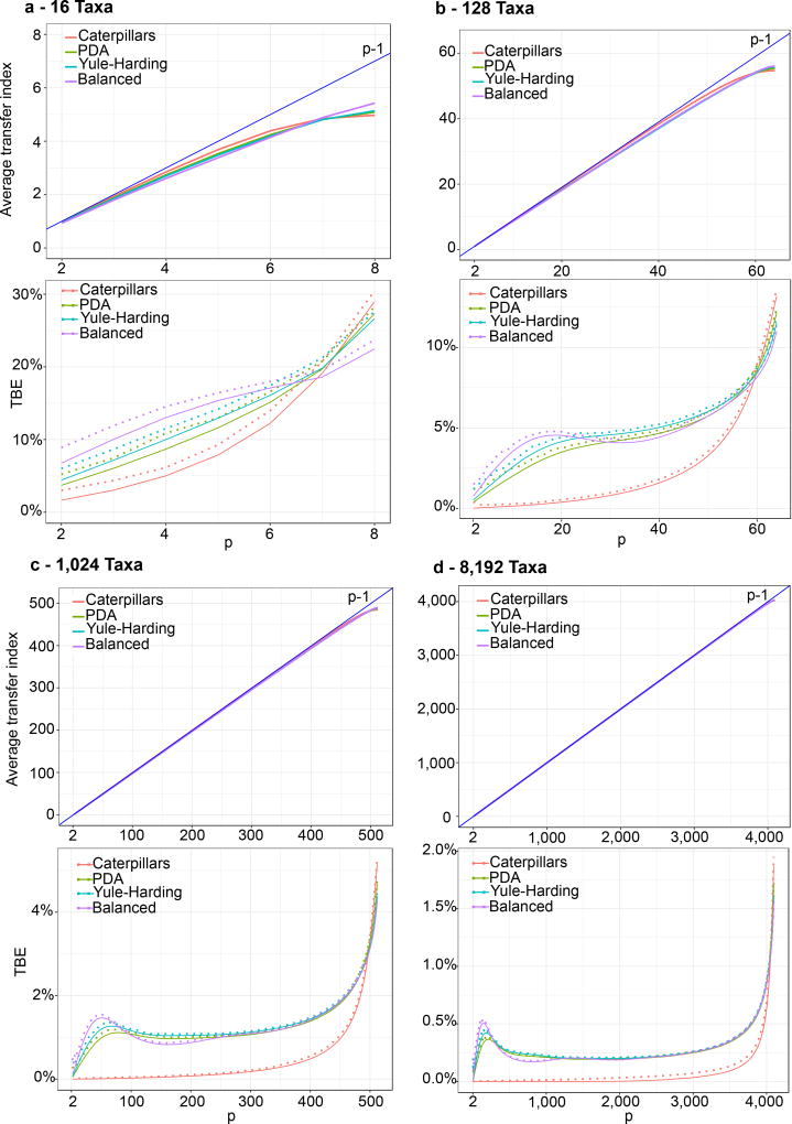
However, these distances fluctuate around their expected values, and their minimum may be lower than the minimum of their individual expectations, especially with small samples (i.e. low number of taxa). We performed computer simulations to measure the extent of this phenomenon and the validity of the E[ϕ(b,T*)] ≈ p − 1 approximation. We used four tree sizes: l = 16, 128, 1,024 and 8,192 taxa, and four models of random phylogenetic trees: caterpillars (fully imbalanced), PDA, Yule-Harding, and perfectly balanced³⁹. For the bipartition b, all possible integer values of p in the [2, l/2] range were used. The number of random “bootstrap” trees was equal to 1,000, and we performed 100 runs per tree size.

Results are displayed in Fig. ED1. With l ≥ 1,024, the average transfer index with random trees is surprisingly close to the upper bound p − 1, and the approximation is already satisfying with l = 128. Moreover, the results are nearly the same for the four random tree models, suggesting that the property holds in a number of settings. As expected, the approximation is better with small p. Indeed, remember that the upper bound p − 1 is obtained with a trivial bipartition b* made of a unique taxon belonging to the light side of b. When a cherry in T* contains two taxa from the light side of b, then ϕ(b,T*) ≤ p − 2. Similar deviations are observed with subtrees in T* containing a large fraction of taxa belonging to the light side of b. The larger p, the higher the probability for such event to occur. Note, however, that large values of p (i.e. p ≈ 2) are relatively rare for most tree models (e.g. Yule-Harding). Looking at the distribution of TBE, we see that having TBE larger than a moderate threshold (say 50%) is very unlikely, even with 16 taxa, thus explaining that TBE rarely supports poor branches with real and simulated data (Fig. 2c–d, ED2–ED3, ED7–ED8).

Software programs, web server

We developed several tools to compute the transfer bootstrap. We first implemented a command line tool in C, “Booster”, available at https://github.com/evolbioinfo/booster. This tool computes TBE as well as FBP supports, and the stability scores of the taxa (globally or per branch). It takes two files as input: (1) a reference tree file in Newick format, and (2) a bootstrap tree file in Newick format, containing all bootstrap trees. A number of software programs can be used to infer trees from MSAs and produce these reference and bootstrap files in the desired format, such as RAxML, FastTree and PhyML, as used in this article, and many others (see examples in Booster GitHub repository).

We also developed “BoosterWeb” (http://booster.c3bi.pasteur.fr), a freely available web interface, which allows users to compute bootstrap supports (TBE and FBP) easily without installing any tool on their own computer. Computations are launched on the Institut Pasteur cluster throughout a Galaxy instance. As for the command line tool, an option is to input reference and bootstrap trees inferred using any phylogenetic program. Another option is to upload an MSA and then run PhyML-SMS⁴⁰ (medium-size data sets) or FastTree (large data sets) to infer the trees. We propose a basic visualization of the resulting tree highlighting highly supported branches at a given threshold. The resulting tree can be uploaded in one-click on iTOL⁴¹ for further manipulation. Moreover, BoosterWeb is self-contained and can be easily installed on any desktop computer (Windows, MacOS, and Linux) by downloading the BoosterWeb executable.

For the sake of reproducibility, all analyses described in this article were implemented in the NextFlow workflow manager⁴², and are accessible along with all our data at https://github.com/evolbioinfo/booster-workflows. The software programs that we developed to manipulate data are available for download at http://github.com/fredericlemoine/goalign and http://github.com/fredericlemoine/gotree, for manipulating alignments and trees, respectively.

Mammal dataset and analyses

We downloaded all aligned mammals COI-5P amino-acid sequences from the Barcode of Life Data System (BOLD - http://www.barcodinglife.org - date of access: September 2015). We removed all sequences shown to be identical among several species, kept one sequence per species (several gene versions are available for some species, but no paralogs), and converted the resulting multiple alignment (1,449 sequences, 527 sites) into FASTA format. This alignment was sub-sampled to study the impact of tree size. We randomly drew 8 samples with 1/8th of the sequences (i.e. 181) and 64 samples with 1/64th of the sequences (i.e. 22). We then generated 1,000 bootstrap alignments for the full alignment and each of the 72 sub-sampled alignments by drawing sites with replacement.

We used FastTree³⁴ (options: -nopr –nosupport –wag –gamma) to infer trees from each of these reference (1+8+64=73) and bootstrap (73,000) alignments. To ensure that the results and conclusions were independent of the tree inference method, we also performed the same analyses using RAxML with rapid bootstrap¹⁷ (options –f a –m PROTGAMMA –c 6 –T 10 –p $RANDOM –x $RANDOM -#1000). The FBP and TBE supports for the (73 × 2) reference trees were computed using Booster (command-line version written in C). All trees were drawn using iTOL and are available on Booster GitHub repository, along with the sequence alignments. To assess whether rogue taxa removal improves FBP supports, we ran RAxML rogue-detection tool²⁴ (options –J MR_DROP –z bootstrap_trees –m PROTGAMMAWAG -c 6 -T 4) and recomputed FBP supports without the detected taxa.

The FastTree and RAxML complete tree topologies were compared to the NCBI taxonomy (https://www.ncbi.nlm.nih.gov/taxonomy), which was converted to Newick format and reduced to the 1,444 taxa common to both our alignment and the NCBI taxonomy. This NCBI tree is not fully resolved and summarizes common belief about the evolutionary history of mammals, resulting from a number of phylogenetic studies based on numerous markers. The unresolved part of the NCBI tree (~4.35 descendants per node on average, instead of 2 for a fully-resolved tree) corresponds to the unknown or uncertain part of that history. To cope with uncertainty, we used quartets to compare the (fully resolved) inferred trees to the NCBI tree. A quartet is a tree topology with 4 taxa; AB|CD is the standard notation for quartets, indicating that taxa A and B form a cherry separated by an internal branch from the cherry formed by C and D; a quartet is unresolved when the 4 taxa are connected to a single central node. A bipartition b induces a quartet AB|CD when A and B belong to the same side of b, and C and D to the other side. We used tqDist⁴³ to count the number of quartets induced by the reference branches, which appeared to be contradictory with the quartets induced by the NCBI tree and its bipartitions; for example, AB|CD was found in the studied branch, while AC|BD was found in the NCBI tree. Unresolved quartets of the NCBI tree were not counted as contradictory, as they represent an unknown evolutionary truth and the inferred resolution could be correct. Such an approach would be difficult to implement with the transfer distance. The number of contradicted quartets was divided by the total number of quartets induced by the studied branch, to obtain a normalized measurement in the [0, 1] range (0: no contradiction; 1: all induced quartets are contradicted). We used the same approach to check the accuracy of the FastTree and RAxML tree topologies, comparing the whole set of quartets induced by the inferred tree to those induced by the NCBI tree.

HIV dataset and analyses

From the HIV database (https://www.hiv.lanl.gov/content/index) we retrieved pol sequences of the nine “pure” subtypes of HIV-1 group M, corresponding to positions 2258-3300 relative to the HXB2 reference strain (access date: September 2014). The “one sequence per patient” option was used, and we randomly selected samples of the over-sampled subtypes (A1, B, C, D, and G), resulting in a final dataset of 9,147 sequences. These sequences are annotated as “pure” (i.e. non-recombinant) in the database, using a fast filtering approach. However, 48 recombinant sequences were still detected using the standalone version of jpHMM³⁷ (version: March 2015; options: -v HIV, with default input and priors). These 48 sequences were kept in the analyses to study the impact of recombinant sequences, as their presence is inevitable in any HIV dataset. jpHMM was also used to annotate the whole set of sequences depending on their subtype or recombinant status.

Sequences were aligned using MAFFT⁴⁴ (version: 7.0; default parameters) along with the HXB2 reference strain. Codon positions associated with major drug resistance mutations were removed prior to tree inference, resulting in an alignment of 1,043 DNA sites (R source code available at https://github.com/olli0601/big.phylo). This alignment was sub-sampled to study the impact of tree size. We randomly drew 16 samples with 1/16th of the sequences (i.e. 571), and 256 samples with 1/256th of the sequences (i.e. 35). Then, we generated 1,000 bootstrap alignments for the full alignment and each of the 272 sub-sampled alignments, by drawing sites with replacement.

We used FastTree³⁴ (options: -nopr –nosupport –gtr –nt -gamma) to infer trees from each of these reference (1+16+256=273) and bootstrap (273,000) alignments. The FBP and TBE supports for the 273 reference trees were computed using Booster (command-line version written in C). All trees were drawn using iTOL (http://itol.embl.de/) and are available on the Booster-workflows GitHub repository, along with the sequence alignments. The instability score was computed considering the reference branches with TBE >70% (the signal becomes noisy when incorporating branches with lower supports in the calculation, as these branches may be erroneous and thus non-informative about taxon stability). For every taxon, the instability score is equal to the average number of times it has to be transferred to recover these branches from the bootstrap trees, divided by the number of these branches.

The most representative clades for each of the subtypes in the reference trees (Fig. 1, ED5) were obtained by minimizing the transfer distance. For example, in Fig. 1 with the full dataset, we obtained a clade very close to subtype B, with 3,559 taxa, 2 wrong taxa (i.e. non-B), and all B taxa included (i.e. 3,557 taxa, 0 missing).

A similar approach was used for the regional variants of subtype C, which is responsible for approximately 50% of the HIV-1 infections in the world. Three monophyletic variants of subtype C have been identified by phylogenetic analysis in East Africa⁴⁵, South America⁴⁶, and India⁴⁷. Moreover, the South American epidemics was shown to originate from the East African cluster⁴⁵. To identify these variants in the inferred trees (Fig. 1, ED5) we again used the transfer distance. Following previous references^45–47, we extracted three groups of C sequences from the whole dataset, based on their geographic origins: East Africa (EA 440 sequences = Burundi 288 + Djibouti 1 + Ethiopia 9 + Kenya 41 + Somalia 1 + Sudan 11 + Tanzania 78 + Uganda 11); India (IND 154 sequences = India 133 + Nepal 13 + Myanmar 8); and South America (SA 14 sequences = Brazil 12 + Uruguay 1 + Argentina 1). We then searched for the tree clades being closer to these three sets of sequences. The SA sequences were not accounted for in transfer distance computations when searching for the EA clade, as they originate from EA. Moreover, we checked that no neighbouring, nearly-optimal clade was supported by FBP. In all three cases, we found clades closely related to the sequence sets. As expected, the SA clade was included in the EA clade. The features of these clades are displayed in Fig. 1 and ED5. The fractions correspond to the number of studied sequences included in these clades, versus the total number of such sequences in the whole dataset (e.g. 360 EA sequences in the EA clade in Fig. 1, among 440 in the whole tree). The “wrong” sequences were expected in most cases. For example, the IND clade (167 sequences, 143 from IND among 154 in the whole tree) contains 19 sequences from China corresponding to the spread of the virus in Asia via heroin trafficking routes⁴⁷.

Simulated data and analyses

The aim of these simulation experiments was to check that the results observed with the mammal and HIV-1 datasets are reproducible and quantifiable when the simulation conditions and correct tree are known, notably regarding the support of poor branches and the ability to detect rogue taxa. Simulated data mimicked the mammal dataset. We used the tree inferred by PhyML⁴⁸ (options: -b 0 -m WAG -a e –t e -o tlr -d aa) from the full COI-5P protein alignment with 1,449 taxa. Protein sequences were evolved along this tree using INDELible⁴⁹, which was launched with options and parameter values derived from the PhyML analysis, and similar to the experiments conducted by Aberer et al.²⁴ to assess the accuracy of rogue-taxon detection:

• Length of the root sequence: 250 AAs;

• Substitution model: WAG;

• Amino-acid frequencies estimated from the COI-5P alignment;

• Rates across-sites model: 4 gamma categories with ‘alpha’ = 0.441 and no invariant sites;

• Indel model: ‘power law’, ‘parameter’ = 1.5, ‘indel max size’ = 5, and ‘indel rate’ = 0.02.

In this manner, we obtained a first “non-noisy” MSA of length ~500 with ~50% gaps. Noise was added to this MSA to mimic rogue taxa and homoplasy. We shuffled the amino acids vertically for 50% of the sites (MSA columns), thus making these sites homoplasic. For 5% of the sequences (MSA rows), 25% additional sites were shuffled vertically, thus making these sequences unstable and “rogue”, as they contain half of the phylogenetic signal compared to the 95% others. Both noisy and non-noisy MSAs were used to compare FBP and TBE. To measure the effect of tree size, both MSAs (comprising 1,449 sequences) were sampled to obtain 8 MSAs with 181 sequences (~1/8 of the full sequence set) and 64 MSAs with 22 sequences (~1/64 of the full sequence set). For each of these reference MSAs we sampled with replacement 1,000 pseudo-alignments to compare the two bootstrap methods. All trees were inferred using FastTree (options: -nopr -nosupport -wag -gamma). Just as with the mammal dataset, we computed, for each of the branches in the reference trees, the percentage of quartet-based conflicts with the correct (PhyML) tree used to generate the data. We also computed the instability score of all taxa in the complete noisy MSA, using only the branches with TBE>70%.

In order to check the repeatability of FBP and TBE, we generated 1,000 noisy MSAs using the same phylogenetic tree, simulation procedure and set of rogue taxa as the reference noisy MSA (1,449 sequences, ~500 sites, ~50% gaps). We then compared the branch supports of the inferred branches computed using the pseudo-alignments to those obtained using the simulated MSAs. The bootstrap theory² indicates that both types of supports are close when the sample size is large enough. The goal was thus to check that 500 sites are enough to obtain a good approximation, and that the bootstrap-based and simulation-based supports are clearly correlated (Pearson’s coefficients), as well as the instability score (again computed using branches with TBE>70%). This experiment was performed with FBP and TBE, with both FastTree (options: -nopr -nosupport -wag –gamma) and RAxML (options: -f d -m PROTGAMMAWAG -c 6). Lastly, the same experiment was used to check the validity of the plug-in principle: we compared the FBP and TBE supports of every inferred branch (both FastTree and RAxML), to the presence/absence (1/0) of that branch in the true tree (FBP), and the normalized transfer distance between that branch and the true tree (TBE).

Data and software availability

All our multiple alignments, phylogenetic trees and workflows are available from the Nature web site, as Source Data. This material, along with a Web interface and software programs, is also available from Booster web site and GitHub: http://booster.c3bi.pasteur.fr ; https://github.com/evolbioinfo/booster. The transfer bootstrap is available in several phylogenetic programs: PhyML, SeaView, RaXML-NG and others (see Booster web site).

Extended Data

Fig. ED1. Transfer index expectation and TBE support with random trees.

For each number of taxa (panels (a) to (d)) and random tree model, we compare the transfer index average over 100 runs with the upper-bound p−1 (top graphs). We also compare the average transfer bootstrap support (TBE) to 0, and provide (dashed lines) the maximum value observed among 100 runs, thus approximating the 1% quantile of the distribution (bottom graphs). With l ≥ 1, 024 (c), the average transfer index with random trees is surprisingly close to the upper bound p − 1, and the approximation is already satisfying with l = 128 (b). Moreover, the results are nearly the same for the four random tree models, suggesting that the asymptotic behaviour holds in a number of settings. As expected, the approximation of the transfer index over random bootstrap trees by p − 1 is better with small p. These results explain why moderate TBE supports, for example 70% as used throughout the article, are sufficient to reject poor branches, as a TBE branch support of 70% cannot be observed by chance, even with a small number of taxa (e.g. 16, (a)).

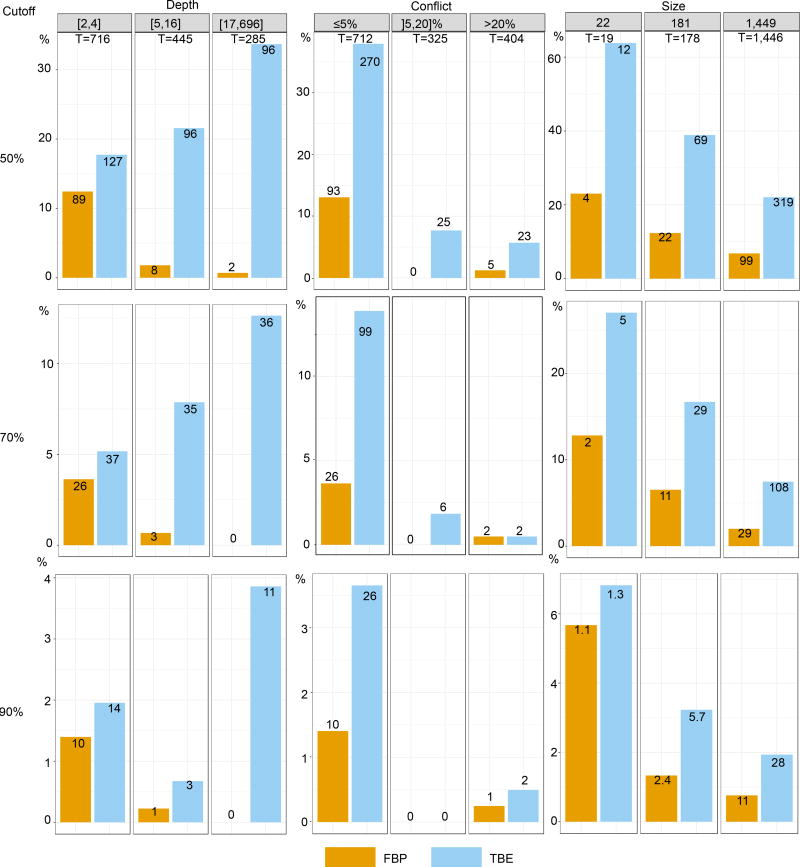
Fig. ED2. Comparison of FBP and TBE – Mammal dataset – FastTree.

Both supports are compared regarding branch depth, quartet conflicts with the NCBI taxonomy, and tree size (see text and notes to Fig. 1 and 2 for explanations). Three support cut-offs are used to select the branches: 50%, 70%, and 90% (e.g. 28 branches among 1,446 have TBE ≥ 90% and 11 have FBP ≥ 90%). The FastTree topology is poor, with 38% of quartets contradicted by the NCBI taxonomy, and 404/1441 branches with contradiction >20%. Despite this difficulty, FBP and TBE perform well as they give supports larger than 70% to a very low number of moderately (]5,20]%) and highly (>20%) conflictual branches. FBP supports very few deep branches, while TBE supports a larger number of them, and is especially useful with large trees. Comparing the three cut-offs, we see that with 50% the selected branches are still weakly contradicted, especially with FBP; as expected, with TBE the fraction of contradicted branches (>5%) is a bit higher but still low (~7%). With 90%, very few branches are selected (~2% with TBE), thus justifying the use of the same 70% threshold for TBE as is standard with FBP.

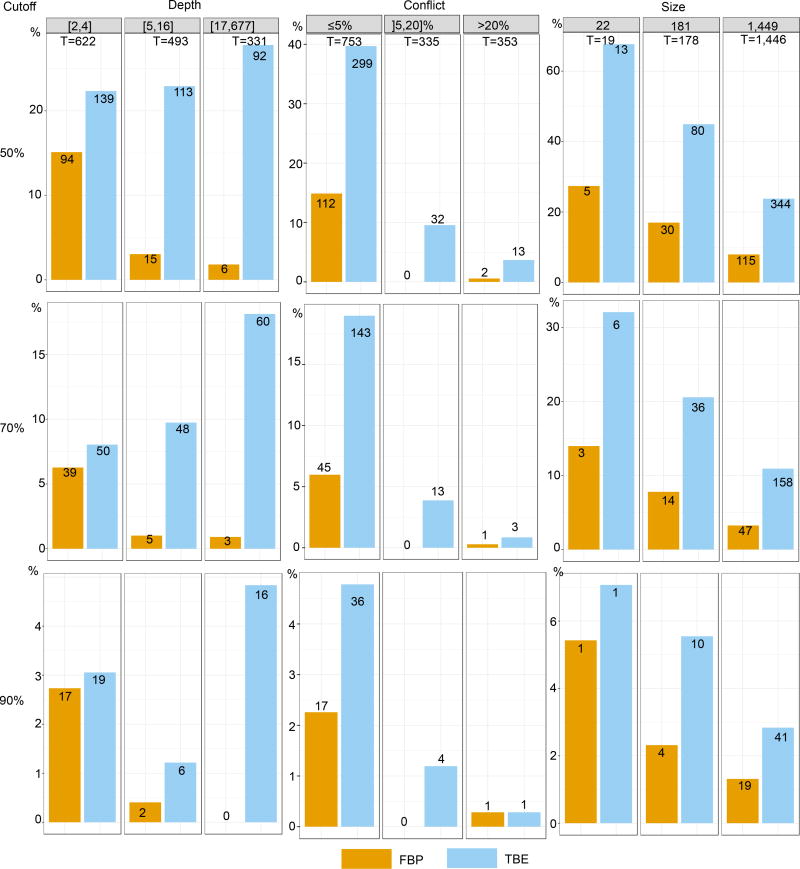
Fig. ED3. Comparison of FBP and TBE – Mammal dataset – RAxML with rapid bootstrap.

Both supports are compared regarding branch depth, quartet conflicts with the NCBI taxonomy, and tree size (see text and notes to Fig. 1 and 2 for explanations). Three support cut-offs are used to select the branches: 50%, 70%, and 90% (e.g. 41 branches among 1,446 have TBE ≥ 90% and 19 have FBP ≥ 90%). The RAxML topology is closer to the NCBI taxonomy than the FastTree topology is (27% versus 38% of contradicted quartets, and 353 versus 404 branches with contradiction >20%, respectively). However, the RAxML topology is still relatively poor, as expected in this type of phylogenetic study based on a unique marker (Fig. 4 and text). Despite this difficulty, FBP and TBE perform well as they give supports larger than 70% to a very low number of moderately (]5,20]%) and highly (>20%) conflictual branches. The supports obtained with RAxML are higher than FastTree’s (47 versus 29 branches with FBP>70%, and 158 versus 108 with TBE>70%, for RAxML and FastTree, respectively). Part of the explanation could be that the RAxML tree is more accurate than that of FastTree, and thus better supported. Another factor is that the rapid bootstrap tends to be more supportive than the standard procedure ^{(e.g. 16)}. Indeed, the rapid bootstrap uses already inferred trees to initiate tree searching, and therefore tends to produce less diverse bootstrap trees than the standard (slower) procedure, which restarts tree searching from the very beginning for each replicate. Despite these differences between FastTree and RAxML with rapid bootstrap, similar conclusions are drawn when comparing FBP and TBE: FBP supports very few deep branches, while TBE supports a larger number of them; TBE is especially useful with large trees; both methods support a very low number of contradicted branches. Comparing the support cut-off, 70% again appears as a good compromise for both FBP and TBE.

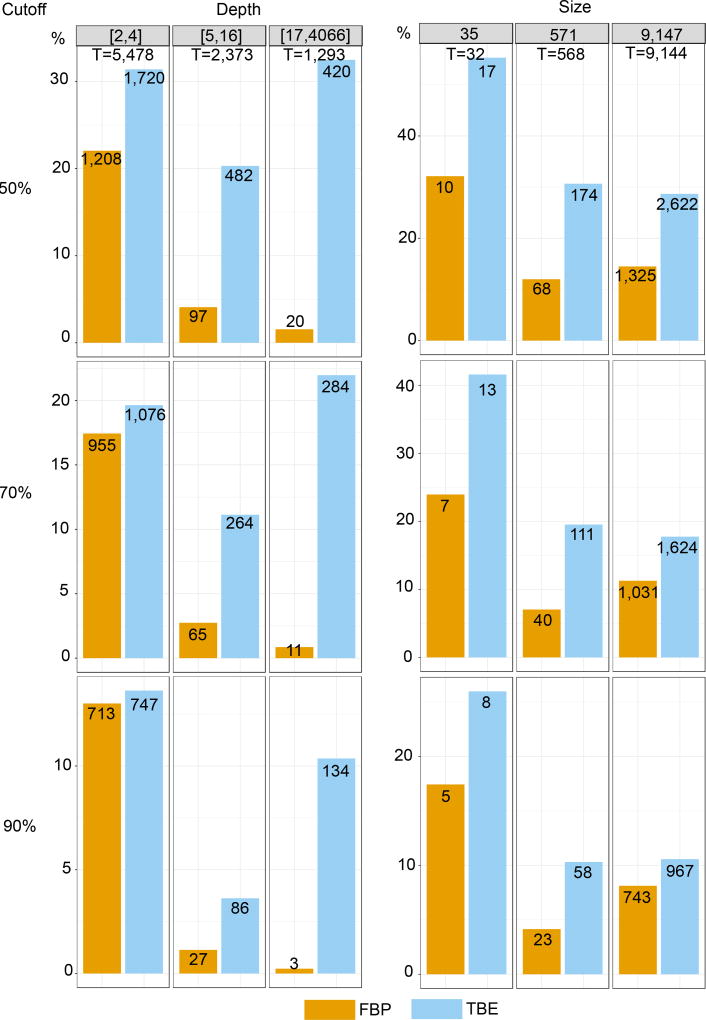
Fig. ED4. Comparison of FBP and TBE – HIV dataset – FastTree.

Both supports are compared regarding branch depth, and tree size (see text and notes to Fig. 1 and 2 for explanations). Three support cut-offs are used to select the branches: 50%, 70%, and 90% (e.g. 1,624 branches among 9,144 have TBE>70% and 1,031 have FBP>70%). Results are mostly similar to those observed with the mammal dataset. Again, we see a major impact of the depth on FBP supports: with the full dataset, less than 1% of the deep (p > 16) branches have FBP support larger than 70%, whereas this percentage is higher than 20% with TBE. The impact of tree size is less pronounced. The fraction of supported branches decreases when the tree size increases from 35 to 571 taxa, but is analogous between 571 and 9,147 taxa. Moreover, the gap between FBP and TBE remains similar, likely due to the very large number of cherries and small clades, where TBE and FBP are nearly equivalent. Regarding the support cut-off, 70% again appears as a good compromise for TBE, though there is no way to evaluate the fraction of supported branches that are actually erroneous. The interpretability of TBE will be a major asset for choosing the support level depending on the phylogenetic question being addressed. Here, as recombinant sequences are inevitable, lower supports than with mammals will likely be acceptable.

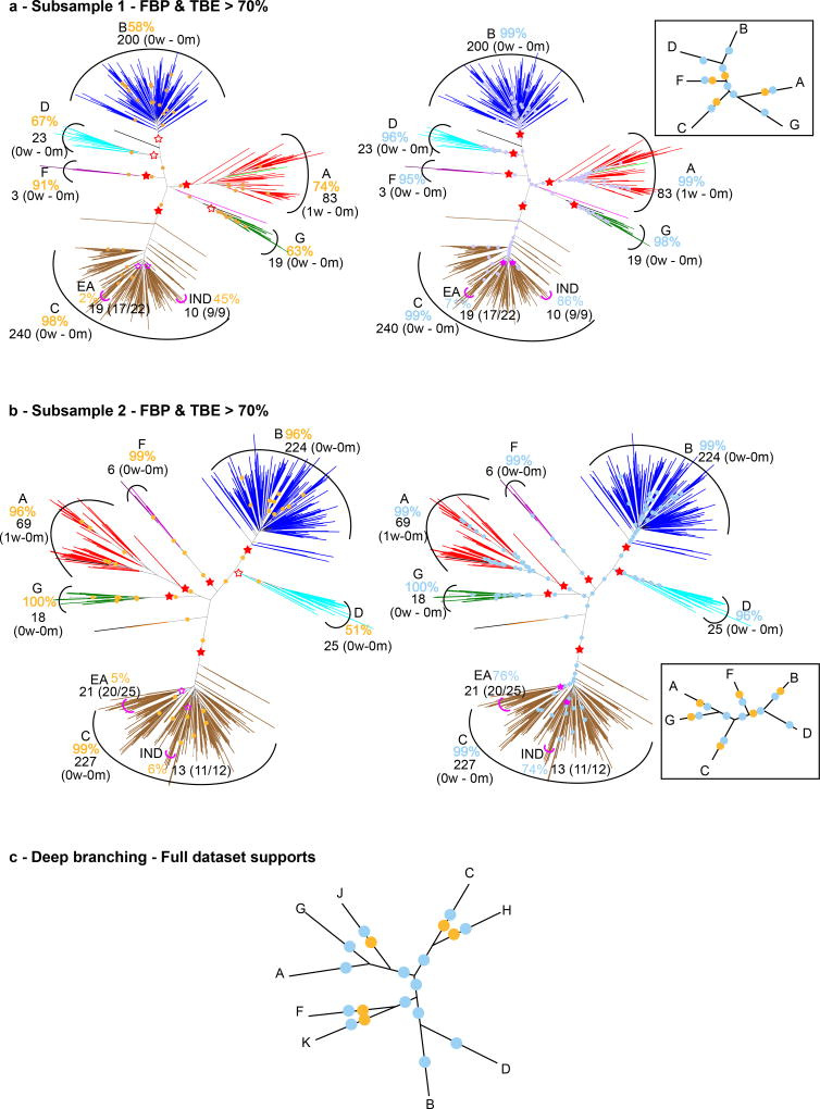
Fig. ED5. Medium-sized HIV datasets, subtype deep branching.

As the taxa were randomly drawn from the full dataset, the supports and findings show some fluctuations. We display the trees obtained with two of the medium-sized datasets in panels (a) and (b); branches with FBP>70%: yellow dots; branches with TBE>70%: blue dots; subtype clades: red stars, filled if support >70% (see Methods and note to Fig. 1 for further details). (c) Deep branching of the subtypes¹⁹ and supports obtained on the full data set (see also Fig. 1). Rare subtypes (H, J, K) are absent in the medium datasets, and the subtype clades are almost perfectly recovered (only 1 wrong taxon in A clade for both trees). FBP supports are higher than with the full dataset (e.g. 58% and 99% for subtype B, versus 3% in Fig. 1). However, some subtype clades have moderate FBP (e.g. D), though the clade matches the subtype perfectly. With TBE, all subtype supports are higher than 95%. The deep branching is the same for all (full, medium) datasets and identical to Hemelaar¹⁹, but not supported by FBP, while TBE is larger than 70% for every branch (or path in Fig. 1). Again, the Indian and East African sub-epidemics of subtype C are supported by TBE, but not by FBP.

Fig. ED6. Distribution of the instability score in HIV recombinants.

We see a clear difference between the distributions of the instability score for the recombinant and non-recombinant sequences, meaning that the approach can be used to detect or confirm the recombinant status of sequences (box quantiles: 25%, 50% and 75%). See text for details.

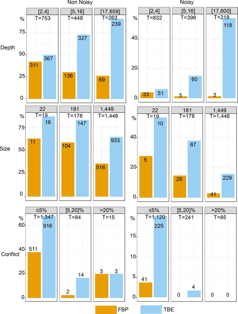
Fig. ED7. Comparison of FBP and TBE – Simulated, non-noisy and noisy data.

Noisy data include rogue taxa and homoplasy, as opposed to non-noisy data. These graphics display the distribution of branches with FPB/TBE support >70%. Both supports are compared regarding branch depth, tree size, and quartet conflicts with the model tree used for simulations (see text and notes to Fig. 1 and 2 for explanations). Results are fully congruent with those obtained with real datasets. TBE supports more deep branches than FBP, especially with noisy data. The effect of tree size is also more visible with noisy MSA, and the number of supported branches with moderate (]5,20]%) and high (>20%) conflict levels is very low, for both FBP and TBE.

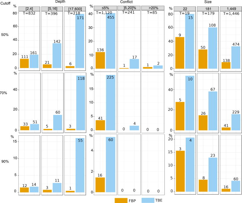
Fig. ED8. Comparison of FBP and TBE at different support cut-offs – Simulated, noisy data.

Comparison of FBP and TBE regarding branch depth, quartet conflicts, and tree size, at different support cut-offs (see text and notes to Fig. 1 and 2 for explanations). A cut-off of 50% seems to be acceptable, as neither FBP nor TBE support highly contradicted branches. But this could be due to the low level of contradiction, compared to real datasets (85 branches with contradiction >20%, versus ~400 with the mammal dataset in Fig. ED2–ED3).

Fig. ED9. Distribution of the instability score in rogue taxa – Simulated, noisy data.

TBE again appears to be useful for detecting and confirming rogue taxa (box quantiles: 25%, 50% and 75%). See text for details.

Fig. ED10. Repeatability and accuracy of FBP and TBE – Simulated data.

The bootstrap theory^1,2 indicates that, with large samples, the supports estimated using bootstrap replicates should be close to supports obtained with datasets of the same size drawn from the same distribution as the original sample. We used simulated data to check that this property holds with protein MSAs of 1,449 taxa and ~500 sites (see text for details). Top panels ((a): FBP, (b): TBE) compare these two supports for all branches in the tree inferred by RAxML from the original MSA. We observe a clear correlation, which is higher for TBE (ρ = 0.85) than for FBP (ρ = 0.75) using Pearson’s linear correlation coefficient, but identical (0.83) using Spearman’s rank coefficient, which is better suited to the discontinuous nature of FBP. These results appear to contradict those of Hillis and Bull⁷ who concluded that the bootstrap is a highly imprecise measure of repeatability. However, they measured the probability to infer the correct tree (not the supports of inferred branches, as consistent in the bootstrap context), and their main result was based on 50 sites, which is likely too low for the bootstrap theory to apply. The bootstrap also relies on the plug-in principle^2,3,6,9 stating that the distribution of the distance between the true tree and the inferred tree can be well-approximated by the distribution of the distance between the inferred and bootstrap trees. Panel (c) measures for every branch b inferred by RAxML from the original MSA, the accuracy of TBE in predicting the topological distance between b and the true tree, as measured using the normalized transfer index. Again, we observe a clear correlation (ρ = 0.74, Spearman’s = 0.70). We performed the same experiment with FBP, seeking to predict the presence/absence (1/0) of the inferred branch in the tree true; a lower but still significant correlation was found (ρ = 0.59, Spearman’s = 0.54). Panel (d) compares using RAxML the performance of simulation-based and bootstrap-based instability scores in detecting rogue taxa; both are nearly identical (TPR: true positive rate; FPR: false positive rate). Table (e) summarizes the results described above, and those of FastTree, which are nearly identical to those of RAxML, except regarding topological accuracy (%correct: fraction of correct branches), where RAxML is again more accurate than FastTree.

References

- 1.Efron B. Bootstrap Methods: Another Look at the Jackknife. Ann. Stat. 1979;7:1–26. [Google Scholar]
- 2.Efron B, Tibshirani RJ. An introduction to the bootstrap. Chapman & Hall, NY; 1993. [Google Scholar]
- 3.Felsenstein J. Confidence limits on phylogenies: an approach using the bootstrap. Evolution. 1985;39:783–791. doi: 10.1111/j.1558-5646.1985.tb00420.x. [DOI] [PubMed] [Google Scholar]
- 4.Van Noorden R, Maher B, Nuzzo R. The top 100 papers. Nature. 2014;514:550–553. doi: 10.1038/514550a. [DOI] [PubMed] [Google Scholar]
- 5.Sanderson MJ. Objections to bootstrapping phylogenies: A critique. Syst. Biol. 1995;44:299–320. [Google Scholar]
- 6.Holmes S. Bootstrapping Phylogenetic Trees: Theory and Methods. Stat. Sci. 2003;18:241–255. [Google Scholar]
- 7.Hillis DM, Bull JJ. An empirical test of bootstrapping as a method for assessing confidence in phyogenetic analysis. Syst. Biol. 1993;42:182–192. [Google Scholar]
- 8.Felsenstein J, Kishino H. Is there something wrong with the bootstrap on phylogenies a reply to hillis and bull. Syst. Biol. 1993;42:193–200. [Google Scholar]
- 9.Efron B, Halloran E, Holmes S. Bootstrap confidence levels for phylogenetic trees. Proc. Natl. Acad. Sci. 1996;93:7085–7096. doi: 10.1073/pnas.93.14.7085. [DOI] [PMC free article] [PubMed] [Google Scholar]
- 10.Susko E. Bootstrap support is not first-order correct. Syst. Biol. 2009;58:211–223. doi: 10.1093/sysbio/syp016. [DOI] [PubMed] [Google Scholar]
- 11.Zharkikh A, Li WH. Estimation of Confidence in Phylogeny: The Complete-and-Partial Bootstrap Technique. Mol. Phyl. Evol. 1995;4:44–63. doi: 10.1006/mpev.1995.1005. [DOI] [PubMed] [Google Scholar]
- 12.Susko E. First-order correct bootstrap support adjustments for splits that allow hypothesis testing when using maximum likelihood estimation. Mol. Biol. Evol. 2010;27:1621–1629. doi: 10.1093/molbev/msq048. [DOI] [PubMed] [Google Scholar]
- 13.Soltis DE, Soltis PS. Applying the Bootstrap in Phylogeny Reconstruction. Stat. Sci. 2003;18:256–267. [Google Scholar]
- 14.Huelsenbeck J, Rannala B. Frequentist Properties of Bayesian Posterior Probabilities of Phylogenetic Trees Under Simple and Complex Substitution Models. Syst. Biol. 2004;53:904–913. doi: 10.1080/10635150490522629. [DOI] [PubMed] [Google Scholar]
- 15.Anisimova M, Gascuel O. Approximate Likelihood-Ratio Test for Branches: A Fast, Accurate, and Powerful Alternative. Syst. Biol. 2006;55:539–552. doi: 10.1080/10635150600755453. [DOI] [PubMed] [Google Scholar]
- 16.Anisimova M, Gil M, Dufayard JF, Dessimoz C, Gascuel O. Survey of branch support methods demonstrates accuracy, power, and robustness of fast likelihood-based approximation schemes. Syst. Biol. 2011;60:685–699. doi: 10.1093/sysbio/syr041. [DOI] [PMC free article] [PubMed] [Google Scholar]
- 17.Stamatakis A, Hoover P, Rougemont J. A Rapid Bootstrap Algorithm for the RAxML Web Servers. Syst. Biol. 2008;57:758–771. doi: 10.1080/10635150802429642. [DOI] [PubMed] [Google Scholar]
- 18.Minh BQ, Nguyen MAT, Von Haeseler A. Ultrafast approximation for phylogenetic bootstrap. Mol. Biol. Evol. 2013;30:1188–1195. doi: 10.1093/molbev/mst024. [DOI] [PMC free article] [PubMed] [Google Scholar]
- 19.Hemelaar J. The origin and diversity of the HIV-1 pandemic. Trends Mol. Med. 2012;18:182–192. doi: 10.1016/j.molmed.2011.12.001. [DOI] [PubMed] [Google Scholar]
- 20.Sanderson MJ, Shaffer HB. Troubleshooting Molecular Phylogenetic Analyses. Annu. Rev. Ecol. Syst. 2002;33:49–72. [Google Scholar]
- 21.Wilkinson M. Majority-rule reduced consensus trees and their use in bootstrapping. Mol. Biol. Evol. 1996;13:437–444. doi: 10.1093/oxfordjournals.molbev.a025604. [DOI] [PubMed] [Google Scholar]
- 22.Thorley JL, Wilkinson M. Testing the Phylogenetic Stability of Early Tetrapods. J. Theor. Biol. 1999;200:343–344. doi: 10.1006/jtbi.1999.0999. [DOI] [PubMed] [Google Scholar]
- 23.Thomson RC, Shaffer HB. Sparse Supermatrices for Phylogenetic Inference: Taxonomy, Alignment, Rogue Taxa, and the Phylogeny of Living Turtles. Syst. Biol. 2010;59:42–58. doi: 10.1093/sysbio/syp075. [DOI] [PubMed] [Google Scholar]
- 24.Aberer AJ, Krompass D, Stamatakis A. Pruning rogue taxa improves phylogenetic accuracy: An efficient algorithm and webservice. Syst. Biol. 2013;62:162–166. doi: 10.1093/sysbio/sys078. [DOI] [PMC free article] [PubMed] [Google Scholar]
- 25.Sanderson MJ. Confidence limits on phylogenies: the bootstrap revisited. Cladistics. 1989;5:113–129. doi: 10.1111/j.1096-0031.1989.tb00559.x. [DOI] [PubMed] [Google Scholar]
- 26.Bréhélin L, Gascuel O, Martin O. Using repeated measurements to validate hierarchical gene clusters. Bioinformatics. 2008;24:682–688. doi: 10.1093/bioinformatics/btn017. [DOI] [PubMed] [Google Scholar]
- 27.Charon I, Denoeud L, Guénoche A, Hudry O. Maximum transfer distance between partitions. J. Classif. 2006;23:103–121. [Google Scholar]
- 28.Day WHE. The complexity of computing metric distances between partitions. Math. Soc. Sci. 1981;1:269–287. doi: 10.1109/tpami.1984.4767476. [DOI] [PubMed] [Google Scholar]
- 29.Lin Y, Rajan V, Moret BME. A Metric for Phylogenetic Trees Based on Matching. IEEE/ACM Trans. Comp. Biol. Bioinf. 2012;9:1014–1022. doi: 10.1109/TCBB.2011.157. [DOI] [PubMed] [Google Scholar]
- 30.Künsch HR. The jackknife and the bootstrap for general stationary observations. Annals of Statistics. 1989;17:1217–1241. [Google Scholar]
- 31.Billera LJ, Holmes SP, Vogtmann K. Geometry of the Space of Phylogenetic Trees. Adv. Appl. Math. 2001;27:733–767. [Google Scholar]
- 32.Kumar S, Filipski AJ, Battistuzzi FU, Kosakovsky Pond SL, Koichiro T. Statistics and Truth in Phylogenomics. Mol. Biol. Evol. 2012;29:457–472. doi: 10.1093/molbev/msr202. [DOI] [PMC free article] [PubMed] [Google Scholar]
- 33.Truszkowski J, Goldman N. Maximum Likelihood Phylogenetic Inference is Consistent on Multiple Sequence Alignments, with or without Gaps. Syst Biol. 2016;65:328–333. doi: 10.1093/sysbio/syv089. [DOI] [PMC free article] [PubMed] [Google Scholar]
- 34.Price MN, Dehal PS, Arkin AP. FastTree 2 - Approximately maximum-likelihood trees for large alignments. PLoS One. 2010;5:e9590. doi: 10.1371/journal.pone.0009490. [DOI] [PMC free article] [PubMed] [Google Scholar]
- 35.https://www.ncbi.nlm.nih.gov/taxonomy, date of access: April 2016, available from Booster GitHub repository https://github.com/evolbioinfo/booster
- 36.Grenfell BT, Pybus OG, Gog JR, Wood JL, Daly JM, Mumford JA, Holmes EC. Unifying the Epidemiological and Evolutionary Dynamics of Pathogens. Science. 2004;303:327–332. doi: 10.1126/science.1090727. [DOI] [PubMed] [Google Scholar]
- 37.Schultz AK, et al. jpHMM: Improving the reliability of recombination prediction in HIV-1. Nuc. Acids Res. 2010;38:1059. doi: 10.1093/nar/gkp371. [DOI] [PMC free article] [PubMed] [Google Scholar]
- 38.Robinson DF, Foulds LR. Comparison of phylogenetic trees. Math. Biosci. 1981;53:131–147. [Google Scholar]
- 39.Semple C, Steel MA. Phylogenetics. Oxford University Press; Oxford, UK: 2003. [Google Scholar]
- 40.Lefort V, Longueville JE, Gascuel O. SMS: Smart Model Selection in PhyML. Mol. Biol. Evol. 2017;34:2422–2424. doi: 10.1093/molbev/msx149. [DOI] [PMC free article] [PubMed] [Google Scholar]
- 41.Letunic I, Bork P. Interactive tree of life (iTOL) v3: an online tool for the display and annotation of phylogenetic and other trees. Nuc. Acids Res. 2016;44:W242–W245. doi: 10.1093/nar/gkw290. [DOI] [PMC free article] [PubMed] [Google Scholar]
- 42.Di Tommaso P, et al. Nextflow enables reproducible computational workflows. Nat. Biotech. 2017;35:316–319. doi: 10.1038/nbt.3820. [DOI] [PubMed] [Google Scholar]
- 43.Sand A, et al. TqDist: A library for computing the quartet and triplet distances between binary or general trees. Bioinformatics. 2014;30:2079–2080. doi: 10.1093/bioinformatics/btu157. [DOI] [PubMed] [Google Scholar]
- 44.Katoh K, Standley DM. MAFFT multiple sequence alignment software version 7: Improvements in performance and usability. Mol. Biol. Evol. 2013;30:772–780. doi: 10.1093/molbev/mst010. [DOI] [PMC free article] [PubMed] [Google Scholar]
- 45.Delatorre EO, Bello G. Phylodynamics of HIV-1 Subtype C Epidemic in East Africa. PLoS One. 2012;7:e41904. doi: 10.1371/journal.pone.0041904. [DOI] [PMC free article] [PubMed] [Google Scholar]
- 46.Soares Ma, et al. A specific subtype C of human immunodeficiency virus type 1 circulates in Brazil. AIDS. 2003;17:11–21. doi: 10.1097/00002030-200301030-00004. [DOI] [PubMed] [Google Scholar]
- 47.Siddappa NB, et al. Identification of subtype C human immunodeficiency virus type 1 by subtype-specific PCR and its use in the characterization of viruses circulating in the southern parts of India. J. Clin. Microbiol. 2004;42:2742–2751. doi: 10.1128/JCM.42.6.2742-2751.2004. [DOI] [PMC free article] [PubMed] [Google Scholar]
- 48.Guindon S, et al. New Algorithms and Mehtods to Estimate Maximum-Likelihood Phylogenies: Asessing the Performance of PhyML 3.0. Syst. Biol. 2010;59:307–321. doi: 10.1093/sysbio/syq010. [DOI] [PubMed] [Google Scholar]
- 49.Fletcher W, Yang Z. INDELible: A flexible simulator of biological sequence evolution. Mol. Biol. Evol. 2009;26:1879–1888. doi: 10.1093/molbev/msp098. [DOI] [PMC free article] [PubMed] [Google Scholar]
Associated Data
This section collects any data citations, data availability statements, or supplementary materials included in this article.