cgDNAweb: a web interface to the cgDNA sequence-dependent coarse-grain model of double-stranded DNA

Abstract

The sequence-dependent statistical mechanical properties of fragments of double-stranded DNA is believed to be pertinent to its biological function at length scales from a few base pairs (or bp) to a few hundreds of bp, e.g. indirect read-out protein binding sites, nucleosome positioning sequences, phased A-tracts, etc. In turn, the equilibrium statistical mechanics behaviour of DNA depends upon its ground state configuration, or minimum free energy shape, as well as on its fluctuations as governed by its stiffness (in an appropriate sense). We here present cgDNAweb, which provides browser-based interactive visualization of the sequence-dependent ground states of double-stranded DNA molecules, as predicted by the underlying cgDNA coarse-grain rigid-base model of fragments with arbitrary sequence. The cgDNAweb interface is specifically designed to facilitate comparison between ground state shapes of different sequences. The server is freely available at cgDNAweb.epfl.ch with no login requirement.

INTRODUCTION

Sequence-dependent shape and stiffness of double-stranded DNA (or dsDNA) are believed to be biologically important in contexts such as the positioning of nucleosomes (1–3), indirect readout by DNA-binding proteins (4,5) and other forms of gene regulation (6). The general assumption is that sequence variation significantly affects the equilibrium probability distribution of configurations of dsDNA that is interacting with an enveloping solvent or heat bath. Such statistical mechanical properties of dsDNA can be probed experimentally by a variety of experimental techniques, e.g. minicircle cyclization experiments such as (7–9), nuclear magnetic resonance (NMR) data (10), X-ray crystal structure (11) and a variety of electron, or atomic force, microscopy techniques (12,13). Each experimental approach has its own advantages, disadvantages and limitations. For example the observed crystal structure configuration of the palindromic Dickerson dodecamer (11) is significantly far from satisfying the requisite symmetry conditions that should hold for the equilibrium distribution ground state for any palindromic fragment of dsDNA in solution (14).

The statistical mechanical equilibrium distribution for DNA can also be probed by appropriate averaging over fully atomistic molecular dynamics (or MD) simulations, such as those carried out by the ABC consortium for example (15). Such MD simulations of a few microsecond duration for several tens of different oligomers of 20 bp or so in length (in an appropriately sized explicit solvent box) are now becoming routine with contemporary, widely available, computational resources. But the vast size of sequence space, even for short fragments, means that only a tiny proportion of all sequences can possibly be simulated using MD codes.

For these and other reasons there is considerable interest in developing sequence-dependent coarse-grain dsDNA models of various types. The goal of such models is typically to lower the computational demands so that it is feasible to achieve longer (model) simulation times, or indeed to predict equilibrium (or infinite time) probability distributions directly, and to be able, for example, to scan entire genomes for physically exceptional sequence fragments. The biological importance of the sequence-dependent shape of DNA is attested to by the number of coarse-grain models that have been developed to address the problem, e.g. Olson et al. (16), Savelyev et al. (17), Sayar et al. (18), the 3SPN model (19), Maciejczyk et al. (20), the Martini coarse grain force field (21), Naômé et al. (22), Morriss-Andrews et al. (23) and the oxDNA model (24). There are also some associated web servers, e.g. NAflex (25), web3DNA (26) and DNAshape (27). A more detailed survey can be found in the recent review article (28).

The bane of coarse-grain descriptions is the estimation of a sufficiently accurate set of parameter values for the model. The novelty of the cgDNAweb site introduced here, is that it provides a visual web interface to specifically the cgDNA predictive coarse-grain model (29). In turn, the cgDNA model is itself novel because it is trained on large-scale libraries of MD simulations of the ABC consortium type, and has proven to accurately predict sequence-dependent fine-structure of ground states as observed in (non-training set) MD simulations, and NMR and X-ray crystal structure experimental data (14), including the prediction of non-local sequence-dependence of ground-states. Here, the adjective accurate means that the discrepancies between cgDNA prediction and the experimental or MD observation are substantially less than the variation of data with DNA sequence. Estimating a full cgDNA model parameter set starting from scratch, i.e. from an associated training library of MD simulations, remains a quite computationally intensive task, but there are now a variety of pre-computed cgDNAparamsets available. Four are currently provided within the cgDNAweb interface, with the associated protocols being described in the online cgDNAweb documentation pane. As further parameter sets are made available, they will similarly be described there.

The cgDNA model has been implemented in Matlab/Octave scripts that are themselves freely available for download. Once a particular cgDNAparamset and sequence have been selected, the calculation of both the associated ground state shape, and a stiffness matrix governing fluctuations about the ground state, is a trivial computation of a few seconds at most using the cgDNA Matlab/Octave scripts. However using these scripts involves pre-installing one of the general purpose Matlab or Octave packages, learning the associated interface and general command syntax, and appropriately loading and understanding the cgDNA scripts. The cgDNAweb interface presented here is designed to avoid all of these preliminary steps, and to allow a simple, direct and visual access to the core scientific output predicted by the cgDNA model. The user selects a cgDNAparamset and enters a sequence, then, essentially instantly, has available both a 3D visualization of the corresponding ground state, and plots of the corresponding Curves+ (30) helicoidal coordinates along the ground state. Technically the input data are sent to the server, which make all necessary cgDNA model computations, which are then sent back to the front-end for display, with all 2D and 3D visualization carried out client-side. cgDNAweb also allows downloads (in various formats) of the numerical data for both the cgDNA ground state and the associated cgDNA stiffness matrix. Nevertheless the primary emphasis of cgDNAweb is on various ways to interactively visualize the ground state of the given sequence via either 2D plots or 3D scenes. To facilitate comparison between different sequences (or indeed between different cgDNAparamsets) the cgDNAweb interface allows superimposed visualizations of up to four different cgDNA ground states.

The cgDNA model

The cgDNA model (29) is a sequence-dependent coarse-grain approximation to dsDNA in which each base is assumed to be a rigid body that interacts directly with each of its five nearest neighbour bases (two on the same backbone, and three on the opposite backbone). The inputs to the cgDNA model of a dsDNA oligomer with N base pairs is a sequence S of N letters drawn from the {A,T,C,G} alphabet (corresponding to the bases along the reading or Watson strand in the 5′ → 3′ direction), along with a model parameter set . Various parameter sets are available corresponding either to different mathematical choices in the parameter estimation techniques (31) or to different MD training set data, which in turn can depend on both different MD simulation protocols, or on physically different solvent conditions, e.g. different ion species and concentration. Current parameter sets are all only for the standard AT and CG base pairings, which are assumed throughout, so that the Watson sequence completely specifies the Crick sequence.

The basic outputs of the cgDNA model are the mean and inverse covariance of a Gaussian, or multi-variate normal, probability density function (or PDF) of the form

(1)

where the variable is the Curves+ (30) internal helicoidal coordinates of the configuration, is the partition function (or normalizing constant), are the Curves+ coordinates of the ground state (which is the configuration that minimizes the shifted quadratic free energy in the argument of the exponential) and is a symmetric, positive definite stiffness (or precision or inverse covariance) matrix, which governs the distribution of fluctuations of configurations about the ground state. The physical interpretation of the PDF (1) is as a predictive approximation of the equilibrium, or stationary, distribution of the configurations of a DNA oligomer of any prescribed sequence S interacting stochastically with solvent composed of water and counter ions.

Curves+ coordinates decompose into alternating sextuplets w = (y¹, z¹, y², z², …, z^N − 1, y^N) where each yⁱ are intra-base pair coordinates, (buckle, propeller, opening, shear, stretch, stagger) whilst each zⁱ are inter-base pair (or junction) coordinates (tilt, roll, twist, shift, slide, rise). Each sextuplet has three rotational coordinates followed by three translational coordinates. Within cgDNA, translations are reported in Angstroms, whilst angular variables are treated internally in units of one-fifth radian (which gives good scaling between diagonal entries of the stiffness matrix K corresponding to translational and angular coordinates). The cgDNAweb interface also allows the option of reporting angular variables in the more familiar unit of degrees. We note that Curves+ has its own web server (32), but the services and codes provided there are aimed at post-processing existing data, from either experiment or MD, whereas the cgDNAweb services are predictive based on the cgDNA model.

The nearest-neighbour interaction approximation in the cgDNA model is complemented by the further assumption that the energy of interaction between any two bases depends only on the composition of those two bases (in the {A,T,C,G} alphabet). Taken together, these two assumptions imply that the stiffness matrix K is banded with an 18 × 18 overlapping block structure, with each block depending only on the flanking dinucleotide sequence step context. The total free energy of an oligomer can then be viewed as a summation over such localized junction free energies. However it is a simple consequence of the linear algebra of carrying out such a summation that the ground state has non-local sequence dependence. Physically the non-locality arises due to a frustration that arises because each individual rigid base participates in two base-pair junctions corresponding to its five nearest neighbours (14,29).

Reconstruction of base and base pair frames

The definition of the Curves+ internal helicoidal coordinates includes reconstruction rules for base and base pair frames (R_i, r_i) for i = 1, …, N that respect the Cambridge and Tsukuba conventions (33,34). Here, r_i are the absolute Cartesian coordinates of a reference point in the ith base pair, whilst R_i is the proper rotation matrix that encodes the absolute orientation of the ith base pair frame. Similarly encode the absolute orientation and position of the ith base frames where ± indicates Watson and (appropriately rotated) Crick strand base frames. In order to eliminate an overall translation and rotation of the dsDNA oligomer, in the Curves+ reconstruction rule one base pair frame can be taken to have arbitrary values, and the cgDNAweb interface allows any base pair frame to be assigned the values (I, 0) (i.e. the identity matrix and the zero vector) after which all other frames are uniquely defined. cgDNAweb then provides a 3D visualization of ground state frames in the sense of and (R_i, r_i)(〈w〉), i.e. the base and base pair frames are reconstructed for the expected value of the Curves+ coordinates under the cgDNA PDF (1). We also refer to these particular frames as a ground state configuration.

A Monte Carlo code cgDNAmc is available (35) to evaluate cgDNA ensemble averages of any given function of the coordinates, such as , which is the expected relative displacement between ith and jth base pair frames. Such expectations are related to persistence lengths in various senses, but are not simply expressible in terms of 〈w〉. Currently, the cgDNAweb interface provides only 2D visualization of 〈w〉 itself, along with 3D visualization of the frames (R_i, r_i)(〈w〉) and reconstructed for the ground state coordinates 〈w〉.

Features of the web server

The header of the cgDNAweb page contains an input form for entering the desired sequence by either copy-paste or typing directly (with the syntax that is fully described in the online documentation pane, in particular upper or lower or mixed case, with or without spaces or carriage returns are all allowed, cf. examples below). Hard limits on sequence length are that inputs must be at least 2 bp long and <3K bp. The border of the input form turns red when the input is rejected, either because of length constraints or unrecognized input syntax. Sufficiently long sequences eventually become unwieldy to manipulate interactively in the 3D viewer particularly when visualizing individual atoms, with the practical maximum being hardware and server dependent. For contemporary laptops usually up to 1K bp or more is feasible, which is well beyond scales at which sequence-effects are believed to be biologically pertinent. End effects in ground state reconstructions effectively vanish (i.e. have effects of <1%) only 5 bp or so away from the ends. This is physically reasonable, but it suggests that a practical lower limit for sequence length is ∼10 bp.

Once a sequence has been entered, a pull down menu selects the parameter set to be used, and then the Go button launches the cgDNA model reconstruction on the server. In fact, there are four input forms that can be used independently and in parallel, with visualizations of the corresponding ground state reconstructions all superimposed to facilitate comparison.

Below the header there are five tabs/panes. They provide credit and citation information, basic online documentation, a pane for downloading numerical data of reconstructions (detail of available formats is described in Supplementary Section S1) and most importantly 2D and 3D visualization panes.

The 2D pane provides 12 sub-panels, each with a plot of one of the Curves+ helicoidal coordinates along the ground state of each of the entered sequences. Different colours encode which sequence is being plotted. When the mouse is positioned over a data point in any graph, a pop-up window displays the precise numerical data and local sequence context for each of the ground states being displayed. These 2D plots of helicoidal coordinates provide the most detailed information about ground states for comparatively short sequences. However for longer sequences the plots become harder to read. And for any length sequence it can be difficult to interpret helicoidal coordinates as 3D configurations.

Accordingly the 3D pane provides a 3D scene of the base and base pair frames of the ground states, which can be interactively rotated and zoomed via the mouse. A drop down sub-menu provides various visualization options. For example each base or base pair frame can be visualized as a point, or origin, along with three orthonormal vectors, or as a rectangular box, colour-coded for sequence. In the vector visualization, the base frames follow the Tsukuba convention (33) and are quite close to the associated base pair frame, but the box representation of a base is offset to be a bounding box for the heavy atoms in the base. Similarly each base can instead be visualized using just spheres centred on its heavy atom locations. However there is no additional information in the atom locations; they are merely idealized coordinates with respect to the base frame as specified in the Tsukuba convention. Similarly there is an option to visualize backbones, but they are only a visual aid constructed from a simple interpolation from the base location data. Further technical detail of the visualization options is provided in Supplementary Section S2. When the mouse is clicked on a base, a pop-up window displays the oligomer and strand numbers along with the base composition. Unless your eye is well-trained, it is difficult to perceive significant differences in the 3D visualizations of short fragments, but large overall intrinsic bends in longer sequences are much clearer in the 3D view than in the corresponding 2D plots, cf. Figure 2 for the tandem repeat A-tract sequence described below.

Figure 2.

The 3D visualizations of the ground state configurations of the multiple A-tract, intrinsically bent, sequence (T_6 GCCCG)_9, compared with the homogeneous, intrinsically straight, sequence T_99. See Supplementary Section S3.2 for the 2D and other 3D visualizations of the same two sequence fragments.

Example sequences

The intention is that cgDNAweb should provide visualization of ground states of specific dsDNA sequences of interest to the user. But here we briefly describe some illustrative examples. Interactivity of visualization is we believe important, so that we encourage the reader to actually input the sequences below in the cgDNAweb page. Nevertheless for comparison purposes, static images of both the full 2D and 3D pane outputs of cgDNAweb for each of the two examples described below are provided in Supplementary Section S3, where the cgDNAweb outputs for further example sequences are also briefly discussed.

The Drew-Dickerson dodecamer and a localized palindromic mutation

Input sequences CGCG aA[T]t CGCG and a palindromic mutation CGCG tA[T]a CGCG. The [ ] in the sequence input sets the base pair frames that are aligned in the 3D visualization. Upper and lower case and spaces are all allowed in the input, which are here used to highlight the two, point mutations between the two sequences. For palindromes the propeller variable plotted in Figure 1 is an even function. The same plot shows that the ground state can exhibit rather delocalized differences consequent upon local sequence changes. Further snapshots of cgDNAweb data for this sequence are provided in Supplementary Section S3.1.

Figure 1.

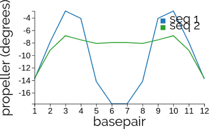
Plots of propeller along the ground states of the Dickerson dodecamer CGCG aA[T]t CGCG (seq 1, blue) and a palindromic mutation CGCG tA[T]a CGCG (seq 2, green), where only the lower case letters changed. The local sequence changes imply non-local changes in the ground state. See Supplementary Section S3.1 for other 2D and 3D visualizations of the same two sequence fragments.

Tandem repeats

Repeating sequence sub-units can be input with a subscript, e.g. nine successive, identical A-tracts each with six successive Ts can be input as (T_6 GCCCG)_9. However the alignment symbol [ ] can only appear once, so the same sequence can also be input as (T_6GCCCG)_4TTT[T]TTGCCCG(T_6 GCCCG)_4 and aligned with a homogeneous poly(T) = T_N sequence of the same length using the syntax T_47[T]T_51. (If the alignment symbol is absent in any input the first base pair frame is taken by default.) We note that in cgDNAweb, sequences such as poly(T) or equivalently (under switch of Watson and Crick strands) poly(A), are homogeneous dsDNA fragments. The 3D view (cf. Figure 2) emphasizes the global bend in the A-tract sequence in contrast to the very straight poly(T), whilst the 2D pane plots provided in Supplementary Section S3.2 reveal that for repeating A-tracts the largest changes in the Curves+ coordinates arise close to the boundary junctions with TG and GT dinucleotide steps. Moreover the ends of the ground state of the homogeneous sequence poly(T) behave differently from the interior, as they should. The poly(T) sequence is also highly exceptional with a very large (negative) value of propeller.

Other examples

The cgDNAweb output for ground states of various other sequences are briefly discussed in Supplementary Section S3.3 three poly-dimer sequences, Sections S3.4 and S3.5 further A-tract examples and comparison with poly(A), Section S3.6 the Widom 601 sequence, and Section S3.7 super-helical structures for tandem repeats.

DISCUSSION

The cgDNAweb page provides an easy-to-use visual interface to the cgDNA predictive model of sequence-dependent ground state configurations of dsDNA. The cgDNA model itself continues to be actively developed in various directions, and the cgDNAweb site will in due course be concomitantly updated. Certainly we intend that the range of available parameter sets will continue to be updated as more MD training library simulations are run. For example, a parameter set with an expanded sequence alphabet including epigenetically modified bases is currently being developed. The current version of the cgDNA model does encompass fluctuations of the dsDNA backbones, but only implicitly. Consequently cgDNAweb only explicitly predicts the ground state configurations of the dsDNA bases, although associated backbones can be approximated via interpolation. However a more refined version of the cgDNA model is currently under development that includes explicit predictions of the backbone ground state via additional frames embedded in the phosphate groups, and we in due course envision an accompanying enhanced version of cgDNAweb.

The cgDNA model predicts both a ground state configuration and a banded stiffness matrix for each input sequence. However cgDNAweb focuses on visualizing the ground state shape in various ways, and only provides the stiffness matrix via download of a file with its numerical entries. There are two reasons for this limitation. First it is not completely clear what are the useful objects to visualize to help in understanding sequence-dependent variations in the stiffness matrix. One, but only one, possibility is to make plots of the eigenvalues of the stiffness matrix, as indicated in Figure 3 (in the scaling with translation variables in Angströms and rotations in one-fifth radians). Such eigenvalue plots could straightforwardly be computed online and provided within cgDNAweb, but for a 1K bp fragment, for which the stiffness matrix is almost 12K by 12K (albeit banded), the intensity of the necessary numerics would substantially slow the response time of the web server. This is our second, and major reason, for not providing such computations within the cgDNAweb interface, and we instead just provide the raw stiffness matrix data to the user, to be post-processed as they wish.

Figure 3.

The cgDNA stiffness matrix for a sequence of length N has 12N − 6 positive eigenvalues, which can be sorted in ascending order and plotted against their index (scaled to always lie in [0,1] to facilitate comparison of spectra for sequences of different lengths). Spectra are here compared for four sequences A_300 (blue), (AT)_150 (green), the Widom 601 positioning sequence (see Supplementary Section S3.6, purple) and the A-tract sequence (A_5 G_5 T_5 C_5 T)_15 (red). The inset in the top left is a magnification of the lower part of the spectra.

It should also be emphasized that the eigenvalues of the stiffness matrix provide only partial information, and that sequence-dependent differences in its eigenvectors, or normal modes, are an equally important ingredient in trying to understand the detail of the physical fluctuations of the fragment. Such differences are harder to visualize and interpret, in part due to the necessary scaling between rotational and translational coordinates. For example, two of the sequences whose eigenvalues are plotted in Figure 3, namely poly(AT) = (AT)_N and poly(A), can be seen to have noticeably, but not very, different eigenvalue spectra. However the same two sequences were included in the cgDNAmc Monte Carlo simulations presented in (35), and poly(AT) was found to have the single shortest (dynamic) persistence length amongst the many thousands of sequences examined, whilst poly(A) had the largest, being 50% longer than that of poly(AT).

SUPPLEMENTARY DATA

Supplementary Data are available at NAR Online.

FUNDING

Swiss National Science Foundation [200020 143613/1 to J.H.M.]. Funding for open access charge: Swiss National Science Foundation [200020 143613/1].

Conflict of interest statement. None declared.

REFERENCES

- 1. Satchwell S.C., Drew H.R., Travers A.A.. Sequence periodicities in chicken nucleosome core DNA. J. Mol. Biol. 1986; 191:659–675. [DOI] [PubMed] [Google Scholar]
- 2. Thåström A., Lowary P.T., Widlund H.R., Cao H., Kubista M., Widom J.. Sequence motifs and free energies of selected natural and non-natural nucleosome positioning DNA sequences. J. Mol. Biol. 1999; 288:213–229. [DOI] [PubMed] [Google Scholar]
- 3. Segal E., Fondufe-Mittendorf Y., Chen L., Thåström A., Field Y., Moore I.K., Wang J.P.Z., Widom J.. A genomic code for nucleosome positioning. Nature. 2006; 442:772–778. [DOI] [PMC free article] [PubMed] [Google Scholar]
- 4. Otwinowski Z., Schevitz R.W., Zhang R.G., Lawson C.L., Joachimiak A., Marmorstein R.Q., Luisi B.F., Sigler P.B.. Crystal structure of trp repressor/operator complex at atomic resolution. Nature. 1988; 335:321–329. [DOI] [PubMed] [Google Scholar]
- 5. Rohs, R., West, S.M., Sosinsky, A., Liu, P., Mann, R.S., Honig B.. The role of DNA shape in protein-DNA recognition. Nature. 2009; 461:1248–1253. [DOI] [PMC free article] [PubMed] [Google Scholar]
- 6. Kim S., Bröstromer E., Xing D., Jin J., Chong S., Ge H., Wang S., Gu C., Yang L., Gao Y.Q. et al. Probing allostery through DNA. Science. 2013; 339:816–819. [DOI] [PMC free article] [PubMed] [Google Scholar]
- 7. Geggier S., Vologodskii A.. Sequence dependence of DNA bending rigidity. Proc. Natl. Acad. Sci. U.S.A. 2010; 107:15421–15426. [DOI] [PMC free article] [PubMed] [Google Scholar]
- 8. Vologodskii A., Frank-Kamenetskii M.D.. Strong bending of the DNA double helix. Nucleic Acids Res. 2013; 41:6785–6792. [DOI] [PMC free article] [PubMed] [Google Scholar]
- 9. Rosanio G., Widom J., Uhlenbeck O.C.. In vitro selection of DNAs with an increased propensity to form small circles. Biopolymers. 2015; 103:303–320. [DOI] [PubMed] [Google Scholar]
- 10. Nikolova E.N., Bascom G.D., Andricioaei I., Al-Hashimi H.M.. Probing sequence-specific DNA flexibility in A-Tracts and pyrimidine-purine steps by nuclear magnetic resonance 13C relaxation and molecular dynamics simulations. Biochemistry. 2012; 51:8654–8664. [DOI] [PMC free article] [PubMed] [Google Scholar]
- 11. Drew H.R., Wing R.M., Takano T., Broka C., Tanaka S., Itakura K., Dickerson R.E.. Structure of a B-DNA dodecamer: conformation and dynamics. Proc. Natl. Acad. Sci. U.S.A. 1981; 78:2179–2183. [DOI] [PMC free article] [PubMed] [Google Scholar]
- 12. Bednar J., Furrer P., Katritch V., Stasiak A., Dubochet J., Stasiak A.. Determination of DNA persistence length by cryo-electron microscopy. separation of the static and dynamic contributions to the apparent persistence length of DNA. J. Mol. Biol. 1995; 254:579–594. [DOI] [PubMed] [Google Scholar]
- 13. Wiggins P.A., van der Heijden T., Moreno-Herrero F., Spakowitz A., Phillips R., Widom J., Dekker C., Nelson P.C.. High flexibility of DNA on short length scales probed by atomic force microscopy. Nat. Nanotechnol. 2006; 1:137–141. [DOI] [PubMed] [Google Scholar]
- 14. Petkevičiūtė D., Pasi M., Gonzalez O., Maddocks J.H.. cgDNA: a software package for the prediction of sequence-dependent coarse-grain free energies of B-form DNA. Nucleic Acids Res. 2014; 42:e153. [DOI] [PMC free article] [PubMed] [Google Scholar]
- 15. Pasi M., Maddocks J.H., Beveridge D., Bishop T., Case D., Cheatham III T., Dans, P., Jayaram B., Lankaš F., Laughton C. et al. ABC: a systematic microsecond molecular dynamics study of tetranucleotide sequence effects in B-DNA. Nucleic Acids Res. 2014; 42:12272–12283. [DOI] [PMC free article] [PubMed] [Google Scholar]
- 16. Olson W. K., Gorin A. A., Lu X. J., Hock L. M., Zhurkin V. B.. DNA sequence-dependent deformability deduced from protein-DNA crystal complexes. Proc. Natl. Acad. Sci. U.S.A. 1998; 95:11163–11168. [DOI] [PMC free article] [PubMed] [Google Scholar]
- 17. Savelyev A., Papoian G.A.. Chemically accurate coarse graining of double-stranded DNA. Proc. Natl. Acad. Sci. U.S.A. 2010; 107:20340–20345. [DOI] [PMC free article] [PubMed] [Google Scholar]
- 18. Sayar M., Avşaroglu B., KabakçIoglu A.. Twist-writhe partitioning in a coarse-grained DNA minicircle model. Phys. Rev. E. 2010; 81:41916. [DOI] [PubMed] [Google Scholar]
- 19. Hinckley D. M., Freeman G. S., Whitmer J. K., de Pablo J. J.. An experimentally-informed coarse-grained 3-site-per-nucleotide model of DNA: structure, thermodynamics, and dynamics of hybridization. J. Chem. Phys. 2013; 139:144903. [DOI] [PMC free article] [PubMed] [Google Scholar]
- 20. Maciejczyk M., Spasic A., Liwo A., Scheraga H.A.. DNA duplex formation with a coarse-grained model. J. Chem. Theory Comput. 2014; 10:5020–5035. [DOI] [PMC free article] [PubMed] [Google Scholar]
- 21. Uusitalo J.J., Ingólfsson H.I., Akhshi P., Tieleman D.P., Marrink S.J.. Martini coarse-grained force field: extension to DNA. J. Chem. Theory Comput. 2015; 11:3932–3945. [DOI] [PubMed] [Google Scholar]
- 22. Naômé A., Laaksonen A., Vercauteren D.P.. A solvent-mediated coarse-grained model of DNA derived with the systematic newton inversion method. J. Chem. Theory Comput. 2014; 10:3541–3549. [DOI] [PubMed] [Google Scholar]
- 23. Morriss-Andrews A., Rottler J., Plotkin S.S.. A systematically coarse-grained model for DNA and its predictions for persistence length, stacking, twist, and chirality. J. Chem. Phys. 2010; 132:035105. [DOI] [PubMed] [Google Scholar]
- 24. Šulc P., Romano F., Ouldridge T.E., Rovigatti L., Doye J.P.K., Louis A.A.. Sequence-dependent thermodynamics of a coarse-grained DNA model. J. Chem. Phys. 2012; 137:135101. [DOI] [PubMed] [Google Scholar]
- 25. Hospital A., Faustino I., Collepardo-Guevara R., González C., Gelpí, J. L., Orozco M.. NAFlex: a web server for the study of nucleic acid flexibility. Nucleic Acids Res. 2013; 41:W47–W55. [DOI] [PMC free article] [PubMed] [Google Scholar]
- 26. Zheng G., Lu X.J., Olson W.K.. Web 3DNA - A web server for the analysis, reconstruction, and visualization of three-dimensional nucleic-acid structures. Nucleic Acids Res. 2009; 37:W240–W246. [DOI] [PMC free article] [PubMed] [Google Scholar]
- 27. Zhou T., Yang L., Lu Y., Dror I., Dantas Machado, A.C., Ghane T., Di Felice, R., Rohs R.. DNAshape: a method for the high-throughput prediction of DNA structural features on a genomic scale. Nucleic Acids Res. 2013; 41:56–62. [DOI] [PMC free article] [PubMed] [Google Scholar]
- 28. Dans P.D., Walther J., Gómez H., Orozco M.. Multiscale simulation of DNA. Curr. Opin. Struct. Biol. 2016; 37:29–45. [DOI] [PubMed] [Google Scholar]
- 29. Gonzalez O., Petkevičiūtė D., Maddocks J.H.. A sequence-dependent rigid-base model of DNA. J. Chem. Phys. 2013; 138:055102. [DOI] [PubMed] [Google Scholar]
- 30. Lavery R., Moakher M., Maddocks J.H., Petkevičiūtė D., Zakrzewska K.. Conformational analysis of nucleic acids revisited: Curves+. Nucleic Acids Res. 2009; 37:5917–5929. [DOI] [PMC free article] [PubMed] [Google Scholar]
- 31. Gonzalez O., Pasi M., Petkevičiūtė D., Glowacki J., Maddocks J.H.. Absolute versus relative entropy parameter estimation in a coarse-grain model of DNA. Multiscale Model. Simul. 2017; 15:1073–1107. [Google Scholar]
- 32. Blanchet C., Pasi M., Zakrzewska K., Lavery R.. CURVES+ web server for analyzing and visualizing the helical, backbone and groove parameters of nucleic acid structures. Nucleic Acids Res. 2011; 39:W68–W73. [DOI] [PMC free article] [PubMed] [Google Scholar]
- 33. Olson W.K., Bansal M., Burley S.K., Dickerson R.E., Gerstein M., Harvey S.C., Heinemann U., Lu X.J., Neidle S., Shakked Z. et al. A standard reference frame for the description of nucleic acid base-pair geometry. J. Mol. Biol. 2001; 313:229–237. [DOI] [PubMed] [Google Scholar]
- 34. Dickerson R., Bansal M., Calladine C., Diekmann S., Hunter W., Kennard O., Lavery R., Nelson H., Olson W., Saenger W. et al. Definitions and nomenclature of nucleic acid structure parameters. J. Mol. Biol. 1989; 205:787–791. [DOI] [PubMed] [Google Scholar]
- 35. Mitchell J.S., Glowacki J., Grandchamp A.E., Manning R.S., Maddocks J.H.. Sequence-dependent persistence lengths of DNA. J. Chem. Theory Comput. 2017; 13:1539–1555. [DOI] [PubMed] [Google Scholar]
Associated Data
This section collects any data citations, data availability statements, or supplementary materials included in this article.