PaRSnIP: sequence-based protein solubility prediction using gradient boosting machine

Abstract

Motivation

Protein solubility can be a decisive factor in both research and production efficiency, and in silico sequence-based predictors that can accurately estimate solubility outcomes are highly sought.

Results

In this study, we present a novel approach termed PRotein SolubIlity Predictor (PaRSnIP), which uses a gradient boosting machine algorithm as well as an approximation of sequence and structural features of the protein of interest. Based on an independent test set, PaRSnIP outperformed other state-of-the-art sequence-based methods by more than 9% in accuracy and 0.17 in Matthew’s correlation coefficient, with an overall accuracy of 74% and Matthew’s correlation coefficient of 0.48. Additionally, PaRSnIP provides importance scores for all features used in training. We observed higher fractions of exposed residues to associate positively with protein solubility and tripeptide stretches with multiple histidines to associate negatively with solubility. The improved prediction accuracy of PaRSnIP should enable it to predict protein solubility with greater reliability and to screen for sequence variants with enhanced manufacturability.

Availability and implementation

PaRSnIP software is available for download under GitHub (https://github.com/RedaRawi/PaRSnIP).

Supplementary information

Supplementary data are available at Bioinformatics online.

1 Introduction

Protein solubility is an important physiochemical property associated with protein expression, and thus is a critical determinant of the manufacturability of therapeutic proteins. Many proteins, when expressed with standard production procedure in Escherichia coli, have low solubility, which reduces their manufacturability. Experimental enhancement of protein solubility is usually achieved through the use of weak promotors, low temperatures, modified growth media, or optimization of other expression conditions (Idicula-Thomas and Balaji, 2005; Magnan et al., 2009).

The main determinant of protein solubility is the amino acid sequence of a protein, its primary structure. Previous studies showed that protein solubility correlates with several amino acid sequence properties, such as the content of charged and turn-forming residues, the level of hydrophobic stretches, the content of different types of residues, or the length of the protein sequence (Bertone et al., 2001; Christendat et al., 2000; Davis et al., 1999; Wilkinson and Harrison, 1991).

This has led to the development of protein solubility predictors based on the amino acid sequence, which were aimed to replace costly wet-lab experiments by preselecting the most promising protein sequences in silico. These predictors include PROSO II (Smialowski et al., 2012), CCSOL (Agostini et al., 2012), SOLpro (Magnan et al., 2009), PROSO (Smialowski et al., 2007), Recombinant Protein Solubility Prediction (RPSP) (Wilkinson and Harrison, 1991), and the scoring card method (SCM) (Huang et al., 2012). Four of these six methods use support-vector machine (SVM) as their core classification model to differentiate between soluble and insoluble proteins. PROSO II method uses a Parzen window model with modified Cauchy kernel and a two-level logistic classifier. CCSOL uses a SVM classifier and identifies coil/disorder, hydrophobicity, β-sheet, and α-helix propensities as most discriminative features. SOLpro uses a two-stage SVM with sequential minimal optimization to build the protein solubility predictor. PROSO tool uses SVM with Gaussian kernel and a Naive Bayes classifier. RPSP performs discriminant analysis with standard Gaussian distribution to distinguish soluble proteins from insoluble ones. Finally, the SCM method that uses a scoring card by utilizing only dipeptide composition to estimate solubility scores of sequences for predicting protein solubility. However, a study that evaluates these algorithms on an independent test set shows that none of these algorithms achieved an accuracy of >65% (Chang et al., 2014), suggesting room for improvement on the accuracy of the solubility predictor.

In this study, we developed PRotein SolubIlity Predictor (PaRSnIP), a protein solubility prediction tool based on a white-box non-linear predictive modeling technique that has been termed gradient boosting machine (GBM) (Friedman, 2001). GBM has been shown to be competitive with black-box non-linear modeling techniques such as SVM (Cortes and Vapnik, 1995). In addition, it has additional advantages, such as providing feature importance even in the case of non-linear classifiers. PaRSnIP was developed using two types of input features to distinguish between soluble and insoluble protein sequences. First, we included features that could be directly determined from the input amino acid sequence, such as frequencies of mono-, di- or tripeptides, absolute charge, or frequencies of turn-forming residues. Second, we used the SCRATCH suite (Magnan and Baldi, 2014) to predict structural information, in particular secondary structure (SS) and relative solvent accessibility (RSA) information, from the amino acid sequence. By using the independent test set developed by Chang et al. (2014), we showed that PaRSnIP outperformed state of the art methods by at least 9% in accuracy. The use of GBM, unlike the use of black-box modeling techniques, enabled us to identify the protein sequence properties that contributed most to distinguish between soluble and insoluble protein sequences. Interestingly, frequencies of amino acid tripeptides and the fraction of exposed residues (FERs) were the most important features.

2 Materials and methods

2.1 Data

In total, 58 689 soluble and 70 954 insoluble sequences, compiled in (Smialowski et al., 2012) were used as the training set. The independent test set of 1000 soluble and 1001 insoluble sequences compiled in Chang et al. (2014) was used as benchmark test set to evaluate the performance of PaRSnIP in comparison to other sequence-based solubility predictors.

We performed two main pre-processing steps to ensure sequence diversity within the training set and between training and independent test set. First, CD-HIT (Fu et al., 2012; Li and Godzik, 2006) was used to reduce sequence redundancy within the training data set with a maximum sequence identity of 90%. Second, we excluded all training set sequences with a sequence identity of 30% or greater to any sequence in the independent test set to establish a representative performance validity by reducing the bias introduced by homologous sequences. The final training dataset was composed of 28 972 soluble and 40 448 insoluble sequences.

2.2 Features

One of the crucial steps in designing a well-performing classifier is the choice of features. Two groups of features were used to train PaRSnIP (Table 1). The first group was composed of features that can be directly derived from protein sequence, including sequence length, molecular weight, and absolute charge. In addition, we calculated the average of hydropathicity (GRAVY) and aliphatic indices (AIs), as well as the fraction of turn-forming residues. Finally, we extracted frequencies of mono- (single amino acid), di- (two consecutive amino acids) and tripeptides (three consecutive amino acids) from the amino acid sequences. The second group of features was structural information predicted from protein sequence using SCRATCH. We predicted three- and eight-state SS information as well as the FER with different RSA cutoffs. Additionally, we multiplied the FER by the hydrophobicity indices of the exposed residues. The majority of features represented the amino acid frequencies, followed by the structural features derived by SCRATCH. In total, we included 8477 features for each amino acid sequence. In contrast to all other sequence-based solubility predictors, we did not perform feature selection to exclude features, but relied on the GBM to prioritize the most important features.

Table 1.

PaRSnIP features

Sequence features	Structural features
Sequence length (1)	Three-state SS (3)
Molecular weight (1)	Eight-state SS (8)
Fraction turn-forming residues (1)	FERs (0–95% cutoffs) (20)
Average hydropathicity (1)
AI (1)	FERs x hydrophobicity of exposed residues
Absolute charge (1)	(0–95% cutoffs) (20)
Frequency Monopeptide (20)
Frequency Dipeptide (400)
Frequency Tripeptide (8000)

Note: The number of features for each component is shown within parentheses.

2.3 Gradient boosting machine

In this work, we utilized a white-box non-linear ensemble technique called GBM (Friedman, 2001; Schapire, 2003) for building a predictive model using the h2o package (Version 3.10.0.8) in R software (https://www.R-project.org/). The family of boosting methods is based on a constructive strategy that the learning procedure will consecutively fit new models to provide a more accurate estimate of the response variable. The principle idea behind this algorithm is to construct the new base-learners to be maximally correlated with the negative gradient of the loss function, associated with the whole ensemble. Any arbitrary loss function ($\text{L}(\text{y},\text{F}(\text{x}\left)\right)$) can be used here. However, if the error function is the classic squared-error loss, the learning procedure would result in consecutive error-fitting. Algorithm 1 briefly summarizes the GBM technique.

Algorithm 1: Gradient boosting machine

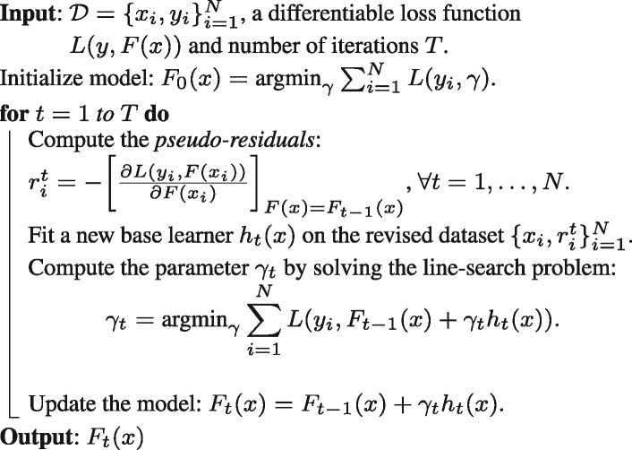
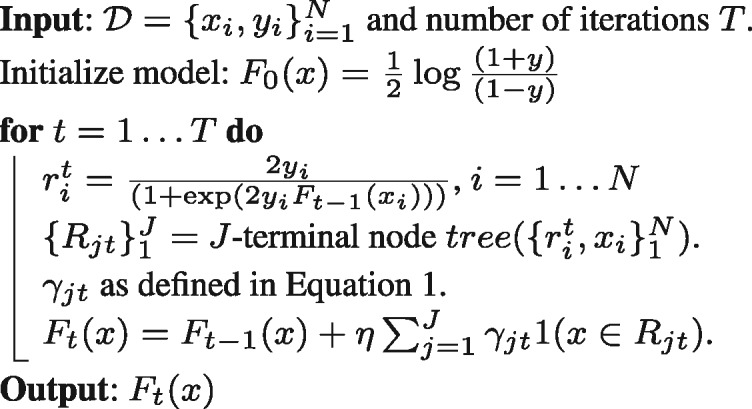
By performing a boosting procedure, we obtained better model performance as this decreased the bias of the model, without increasing variance. We used the L₂-TreeBoost approach as proposed in (Friedman, 2001) to build the GBM model. Here the loss function is negative binomial log-likelihood:

$$L(y,F(x\left)\right)=\text{log}\hspace{0.17em}(1+\text{exp}\hspace{0.17em}(-2yF\left(x\right)\left)\right),y\in \{-1,1\},$$

where $F\left(x\right)=\frac{1}{2}\text{log}\hspace{0.17em}\left[\frac{Pr(y=1|x)}{Pr(y=-1|x)}\right]$. Here $Pr(y=1|x)$ represents the probability of y = 1 given sample x. Similarly, $Pr(y=0|x)$ represents the probability of y = −1 given sample x. Then, the pseudo-residual becomes:

$$r_i^t=-{\left[\frac{\partial L(y_i,F(x_i\left)\right)}{\partial F\left(x_i\right)}\right]}_{F\left(x\right)=F_{t-1}\left(x\right)}=\frac{2y_i}{(1+\text{exp}\hspace{0.17em}(2y_i{F}_{t-1}\left(x_i\right)\left)\right)}$$

The line search then becomes:

$${\gamma }_t={\text{arg}}_{\gamma }\text{min}{\sum }_{i=1}^N\hspace{0.17em}\text{log}\hspace{0.17em}(1+\text{exp}\hspace{0.17em}(-2y_i\left(F_{t-1}\right(x_i)+\gamma h_t(x_i\left)\right)\left)\right)$$

Using regression trees as base learners, we used the idea of separate updates in each terminal node (R_jt) as proposed in (Friedman, 2001):

$${\gamma }_{jt}={\text{arg}}_{\gamma }\text{min}{\sum }_{x_i\in R_{jt}}\hspace{0.17em}\text{log}\hspace{0.17em}(1+\text{exp}\hspace{0.17em}(-2y_i\left(F_{t-1}\right(x_i)+\gamma )\left)\right).$$

However, there is no closed-form solution to the above mentioned equation for optimal line search parameter. Therefore, we approximated it by a single Newton-Raphson (Lindstrom and Bates, 1988) step that leads to:

$${\gamma }_{jt}={\sum }_{x_i\in R_{jt}}\frac{r_i^t}{{\sum }_{x_i\in R_{jt}}\left|r_i^t\right|(2-|r_i^t\left|\right)},$$ (1)

where $r_i^t$ represents the residuals at iteration t. The L₂-TreeBoost approach for two-class likelihood boosting machine is summarized in Algorithm 2.

Algorithm 2:L₂-TreeBoost method for GBM

In Algorithm 2, the function is an indicator function representing whether sample x belongs to terminal region R_jt during the t^th iteration. The parameter η is a regularization parameter which is used to prevent over-fitting and estimated via cross-validation. During each iteration t, the least-squares criterion used to evaluate potential splits of a current terminal region R into two sub-regions (R_l, R_r) was represented as:

$$i^2(R_l,R_r)=I(\varphi )=\frac{w_l{w}_r}{w_l+w_r}{(y_l-y_r)}^2,$$ (2)

where y_l and y_r are the left and right child node responses respectively, and w_l, w_r are proportional to number of elements in region R_l and R_r as shown in (Friedman, 2001). This least-squares criterion (Equation 2) is then considered as the measure of importance ($I(\varphi )$) of the variable/feature ($\varphi$) which maximizes this criterion. Because each feature can cause a split into 2 terminal regions, in the case of J-terminal node tree, we generated importance for J-1 features. Here, the same feature can be used multiple times to generate multiple splits in the J-terminal node tree. In such a case, we summed the importance of such features to get the total contribution ($I(\varphi )$) of each feature ($\varphi$) during iteration t. By using this procedure, we obtained the variable importance scores from the GBM.

2.4 Evaluation metrics

We evaluated the performance of PaRSnIP with several state-of-the-art protein solubility prediction tools using the evaluation metrics prediction accuracy and the correlation coefficient between the predicted and experimentally determined solubility, in particular the Matthews Correlation Coefficient (MCC) during the training phase. We also took into consideration the class-imbalance in the training set and quantify the performance for each class in the independent test set using the following evaluation metrics:

• Sensitivity (Soluble): the ratio between the number of correctly classified instances from soluble class and the total number of instances in the soluble class.

• Sensitivity (Insoluble): the ratio between the number of correctly classified instances from insoluble class and the total number of instances in the insoluble class.

• Selectivity (Soluble): the ratio between the number of correctly classified instances from soluble class and the total number of instances predicted to be in the soluble class.

• Selectivity (Insoluble): the ratio between the number of correctly classified instances from insoluble class and the total number of instances predicted to be in the insoluble class.

• Gain (Soluble): the ratio of Selectivity (Soluble) to the proportion of soluble instances in the full dataset.

• Gain (Insoluble): the ratio of Selectivity (Insoluble) to the proportion of insoluble instances in the full dataset.

3 Results

3.1 Training of PaRSnIP

The training of PaRSnIP included several steps (Fig. 1, top panel). To reduce data redundancy, all training sequences were first clustered with a 90% sequence similarity threshold using CD-HIT. The remaining sequences with a sequence identity of 30% or greater to any sequence in the independent test set were excluded to reduce prediction bias. This resulted in a fairly balanced final training set of 28 972 soluble and 40 448 insoluble sequences. For feature extraction (Fig. 1, middle panel), we extracted from each soluble and insoluble sequence two types of features: (i) those that can be directly derived from the protein sequence, and (ii) structural features determined by the SCRATCH suite (Magnan and Baldi, 2014) using amino acid sequences as input. To train the GBM classifier (Fig. 1, lower panel), given the fact that a GBM classifier is based on several parameters such as the maximum number of trees or number of iterations (T), maximum depth (J) of a tree, sample rate (r), and the regularization parameter η, we performed a hyperparameter optimization by varying these parameters creating a grid of $T\times J\times r\times \eta =288$ combinations, in particular $T\in \{500,1000,1500\},\hspace{0.17em}J\in \{1,3,6,9\},\hspace{0.17em}r\in \{0.1,0.3,0.5\}$, and $\eta \in \{0.001,0.005,0.01,0.05,0.1,0.2,0.3,0.5\}$. We then performed ten-fold cross-validation for each of the combinations. Finally, we selected the GBM classifier that had the maximal ten-fold cross-validation area-under-the-curve, in particular having the parameters T = 500, J = 6, r = 0.3 and $\eta =0.05$. The final classifier had a maximum training accuracy of 0.87 and a maximum MCC of 0.74. A comprehensive training performance comparison of the final GBM classifier to other sequence-based solubility predictors can be found in Supplementary Table S1.

Fig. 1.

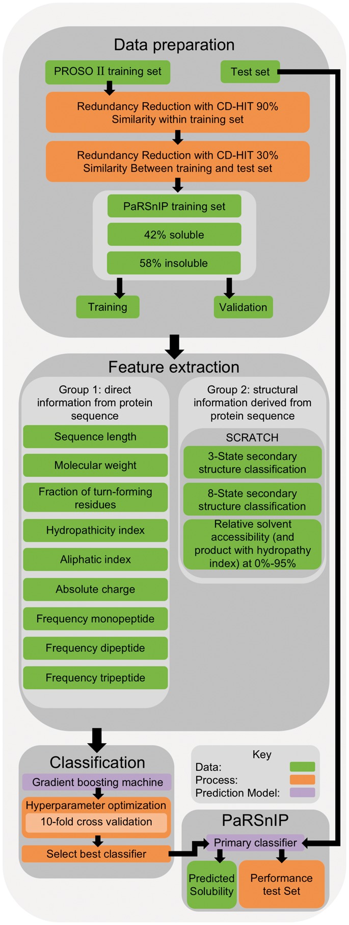
PaRSnIP development flowchart

3.2 Variable importance

An advantage of tree-based machine learning methods, in contrast to black-box modeling techniques such as SVM, is that we can obtain variable importance scores for all input features. In Table 2 we listed all features of the final GBM classifier with a relative importance greater than 5%. Four features, in particular FERs with thresholds of 65, 70 and 75%, and frequency of tripeptide IHH, accounted for 33.67% of the relative importance.

Table 2.

PaRSnIP’s most important features with relative importance >5%

	Feature	Relative importance (%)
1	FER_65	9.94
2	Tripeptide_IHH	9.68
3	FER_70	7.50
4	FER_75	6.56

Note: The full list of features with the corresponding relative variable importances can be found in Supplementary Table S2.

The feature with the highest relative importance of 9.94% was FER with a RSA cutoff of 65%. Interestingly, the association between solubility propensity and higher frequencies of FER_65 within a protein was highly significant (P < 0.0001) (Fig. 2a). The features with the third and fourth highest relative importance FER_70 and FER_75 were also highly significantly associated with solubility propensity (P < 0.0001) (Fig. 2c and d). The second most important feature Tripeptide_IHH, frequencies of the amino acid stretch of isoleucine-histidine-histidine, had a relative importance of 9.68%. In contrast to FER_65, FER_70 and FER_75, higher frequencies of tripeptide IHH were significantly associated with insolubility (P < 0.0001) (Fig. 2b). The full list of all features and their corresponding association P-values can be found in Supplementary Table S2.

Fig. 2.

Frequency distribution of top features with relative importance higher than 5% for soluble and insoluble training protein sequences shown as box plots. ($****:$P-value < 0.0001). (a) FER_65, (b) Tripeptide_IHH, (c) FER_70 and (d) FER_75

Next, we analyzed the overall variable importance contribution of all features according to their feature types (see Fig. 3). We assigned feature classes by first merging the features sequence length, molecular weight, fraction of turn-forming residues, average hydropathicity, AI and absolute charge to one class, which we termed Simple class. Further, we combined mono-, di- and tripeptide features into three classes, respectively. The remaining classes were composed of SS, FER and FER including hydrophobicity features, respectively. Interestingly, tripeptide and FER features accounted for >75% of the variable importance (Fig. 3a). However, the inclusion of 8000 tripeptide features led to a tremendous increase in computational cost during GBM model training. Inclusion of 20 FER features had a low computational expense and improved the gain in variable importance, which can be inferred from the relative variable importance bar plots (Fig. 3b), where the sum of the importance contribution is divided by the number of members in the feature class.

Fig. 3.

Bar plots illustrating the variable importance contribution of each class of features. (a) Sum of variable importances according to their feature class. (b) Sum of the contribution of feature classes divided by the number of features in a certain class

3.3 PaRSnIP performance

The prediction performance of PaRSnIP was assessed using an independent test set reported by Chang et al. (2014). We compared PaRSnIP with solubility predictors PROSO II, CCSOL, SOLpro, PROSO, RPSP and SCM. PaRSnIP yielded a prediction accuracy of 74.11% and a MCC of 0.48, outperforming the state-of-the-art method PROSO II by >9% in accuracy and 0.17 in MCC (see Table 3). PaRSnIP achieved balanced values (between 0.73 and 0.75) in sensitivity and selectivity metrics for both soluble and insoluble instances, whereas other predictors were either class biased, or had significantly lower values. In fact, PaRSnIP outperformed all predictors in all evaluation metrics except for the sensitivity (insoluble) metric, where PROSO II achieved a higher value of 0.82 in contrast to 0.75 for PaRSnIP. However, PROSO II uses a classification probability threshold of 0.6, instead of the usual 0.5, which makes the classifier to predict more instances as insoluble. Thus, to test if PaRSnIP was still the better classifier, we recalculated the performance metrics using the same probability threshold of 0.6. We obtained 73.06, 0.48, 0.59, 0.87, 0.82, 0.68, 1.64 and 1.36 for the metrics accuracy, MCC, sensitivity (soluble), sensitivity (insoluble), selectivity (soluble), selectivity (insoluble), gain (soluble) and gain (insoluble), respectively, and outperformed PROSO II in all evaluation metrics (Supplementary Table S3). Finally, we assessed the performance of PaRSnIP using different probability values as threshold (see Table 4). The best performance was achieved when using a probability threshold of 0.5, which was reasonably expected, since the training as well as test sets are balanced.

Table 3.

Prediction performance of PaRSnIP compared with six protein solubility prediction tools

	PaRSnIP	PROSO II	CCSOL	SOLpro	PROSO	RPSP	SCM
Accuracy (%)	74.11	64.35	54.20	59.95	57.85	51.45	59.67
MCC	0.48	0.31	0.08	0.20	0.16	0.03	0.21
Sensitivity (soluble)	0.73	0.46	0.51	0.51	0.54	0.44	0.42
Sensitivity (insoluble)	0.75	0.82	0.57	0.69	0.62	0.59	0.77
Selectivity (soluble)	0.75	0.72	0.54	0.62	0.58	0.52	0.65
Selectivity (insoluble)	0.74	0.60	0.54	0.58	0.57	0.51	0.57
Gain (soluble)	1.50	1.45	1.09	1.24	1.17	1.03	1.30
Gain (insoluble)	1.47	1.21	1.08	1.17	1.15	1.02	1.14

Note: Best performing method in bold. Performance values adopted from Chang et al. (2014).

Table 4.

Prediction performance of PaRSnIP using different probability thresholds

Probability threshold	0.1	0.2	0.3	0.4	0.5	0.6	0.7	0.8	0.9
Accuracy(%)	65.67	66.07	70.01	73.06	74.11	73.06	70.16	65.67	57.27
MCC	0.43	0.41	0.44	0.47	0.48	0.48	0.44	0.38	0.24
Sensitivity (soluble)	0.99	0.97	0.90	0.81	0.73	0.59	0.50	0.38	0.17
Sensitivity (insoluble)	0.32	0.36	0.50	0.65	0.75	0.87	0.91	0.94	0.97
Selectivity (soluble)	0.59	0.60	0.64	0.70	0.75	0.82	0.84	0.86	0.86
Selectivity (insoluble)	0.99	0.91	0.83	0.77	0.74	0.68	0.64	0.60	0.54
Gain (soluble)	1.19	1.20	1.29	1.40	1.50	1.64	1.69	1.72	1.72
Gain (insoluble)	1.97	1.83	1.66	1.55	1.47	1.36	1.29	1.20	1.08

Note: Best performing probability threshold in bold.

4 Discussion

The development of in silico sequence-based protein solubility prediction tools with high accuracy continues to be to be highly sought. In this study, we introduced PaRSnIP, a solubility predictor that uses GBM algorithm and features that represent sequence as well as structural properties of proteins. PaRSnIP outperformed, to the best of our knowledge, all existing sequence-based solubility predictors by >9% in accuracy and >0.17 in MCC.

The superiority of PaRSnIP over other predictors is due to three factors. The first factor is the choice of the machine learning method GBM. The non-linear boosting technique GBM is able to capture non-linear relationships between the features and the dependent vector (solubility classification), which makes its performance comparable to SVMs. Moreover, GBM reduces the bias of the model without increasing the variance, leading to better generalization performance. In addition, GBM has the ability to provide variable importance, making the model interpretable, which is a drawback of black-box non-linear SVMs. The second factor is the choice of features. We included several features that provided information about sequence and structural properties of the protein of interest. Previous tools such as SOLpro included similar features, amongst others mono-, di- and tripeptide stretches as well as FER at threshold 25%. However, application of feature selection prior to the training of their SVM classifier reduces the information used in training the classifier and hence the final prediction strength. In contrast, we included all 8477 features during the model building stage and did not perform feature selection a priori. In general, using this high number of features includes a risk of overfitting the classifier. GBM can reduce the risk of overfitting by generating a variable importance score for each of the feature, and filter out non-essential features that have very low variable importance scores as a pruning step. Finally, we used the largest available protein solubility data set to date, published by the PROSO II developers (Smialowski et al., 2012). The combination of these three factors led to the superiority of PaRSnIP. An additional advantage of applying GBM as classifier modeling technique is that we obtained relative importance values for all included features. The features with the highest relative importance in PaRSnIP were frequencies of FER_65, FER_70, FER_75 and tripeptide IHH. We noticed from the training set that the FERs for the soluble set is significantly higher than the FERs for the insoluble set (see Fig. 2), which is the reason that the FER is a dominant feature of the classifier. We also noticed that the insoluble proteins tend to have higher tripeptides containing multiple histidines. Interestingly, positively charged surface residues and polyhistidine-tags have been previously correlated with protein insolubility, which explained in part the high importance of feature tripeptide IHH (Chan et al., 2013; Woestenenk et al., 2004). The variable importance values for all features (Supplementary Table S2) provided further insights into what determines protein solubility and encourage further tool development, which might include more structural features, as well as longer peptide stretches, or other relevant features.

In this work, we developed PaRSnIP, a novel sequence-based solubility predictor that used GBM technology and features depicting sequence and structural properties of proteins. PaRSnIP not only outperformed all existing sequence-based solubility predictors, but is the first approach that provides feature importance for all features. Hence, PaRSnIP could be applied in several applications, such as to preselect initial targets that are soluble or to alter solubility of target proteins.

References

- Agostini F. et al. (2012) Sequence-based prediction of protein solubility. J. Mol. Biol., 421, 237–241. [DOI] [PubMed] [Google Scholar]
- Bertone P. et al. (2001) SPINE: an integrated tracking database and data mining approach for identifying feasible targets in high-throughput structural proteomics. Nucleic Acids Res., 29, 2884–2898. [DOI] [PMC free article] [PubMed] [Google Scholar]
- Chan P. et al. (2013) Soluble expression of proteins correlates with a lack of positively-charged surface. Sci. Rep., 3, 3333.. [DOI] [PMC free article] [PubMed] [Google Scholar]
- Chang C.C.H. et al. (2014) Bioinformatics approaches for improved recombinant protein production in Escherichia coli: protein solubility prediction. Brief. Bioinformatics, 15, 953–962. [DOI] [PubMed] [Google Scholar]
- Christendat D. et al. (2000) Structural proteomics of an archaeon. Nat. Struct. Biol., 7, 903–909. [DOI] [PubMed] [Google Scholar]
- Cortes C., Vapnik V. (1995) Support-Vector Networks. Mach. Learn., 20, 273–297. [Google Scholar]
- Davis G.D. et al. (1999) New fusion protein systems designed to give soluble expression in Escherichia coli. Biotechnol. Bioeng., 65, 382–388. [PubMed] [Google Scholar]
- Friedman J.H. (2001) Greedy function approximation: a gradient boosting machine. Ann. Stat., 29, 1189–1232. [Google Scholar]
- Fu L. et al. (2012) CD-HIT: accelerated for clustering the next-generation sequencing data. Bioinformatics (Oxford, England), 28, 3150–3152. [DOI] [PMC free article] [PubMed] [Google Scholar]
- Huang H.-L. et al. (2012) Prediction and analysis of protein solubility using a novel scoring card method with dipeptide composition. BMC Bioinformatics, 13(Suppl 1), S3. [DOI] [PMC free article] [PubMed] [Google Scholar]
- Idicula-Thomas S., Balaji P.V. (2005) Understanding the relationship between the primary structure of proteins and its propensity to be soluble on overexpression in Escherichia coli. Prot. Sci., 14, 582–592. [DOI] [PMC free article] [PubMed] [Google Scholar]
- Li W., Godzik A. (2006) Cd-hit: a fast program for clustering and comparing large sets of protein or nucleotide sequences. Bioinformatics (Oxford, England), 22, 1658–1659. [DOI] [PubMed] [Google Scholar]
- Lindstrom M.J., Bates D.M. (1988) Newton-Raphson and EM algorithms for linear mixed-effects models for repeated-measures data. J. Am. Stat. Assoc., 83, 1014. [Google Scholar]
- Magnan C.N., Baldi P. (2014) SSpro/ACCpro 5: almost perfect prediction of protein secondary structure and relative solvent accessibility using profiles, machine learning and structural similarity. Bioinformatics (Oxford, England), 30, 2592–2597. [DOI] [PMC free article] [PubMed] [Google Scholar]
- Magnan C.N. et al. (2009) SOLpro: accurate sequence-based prediction of protein solubility. Bioinformatics (Oxford, England), 25, 2200–2207. [DOI] [PubMed] [Google Scholar]
- Schapire R.E. (2003) The boosting approach to machine learning: an overview In: Nonlinear Estimation and Classification. Springer, New York, New York, USA, pp 149–171. [Google Scholar]
- Smialowski P. et al. (2007) Protein solubility: sequence based prediction and experimental verification. Bioinformatics, 23, 2536–2542. [DOI] [PubMed] [Google Scholar]
- Smialowski P. et al. (2012) PROSO II - a new method for protein solubility prediction. FEBS J., 279, 2192–2200. [DOI] [PubMed] [Google Scholar]
- Wilkinson D.L., Harrison R.G. (1991) Predicting the solubility of recombinant proteins in Escherichia coli. Bio/Technology (Nature Publishing Company), 9, 443–448. [DOI] [PubMed] [Google Scholar]
- Woestenenk E.A. et al. (2004) His tag effect on solubility of human proteins produced in Escherichia coli: a comparison between four expression vectors. J. Struct. Funct. Genomics, 5, 217–229. [DOI] [PubMed] [Google Scholar]
Associated Data
This section collects any data citations, data availability statements, or supplementary materials included in this article.