Robust inference of population structure from next-generation sequencing data with systematic differences in sequencing

Abstract

Motivation

Inferring population structure is important for both population genetics and genetic epidemiology. Principal components analysis (PCA) has been effective in ascertaining population structure with array genotype data but can be difficult to use with sequencing data, especially when low depth leads to uncertainty in called genotypes. Because PCA is sensitive to differences in variability, PCA using sequencing data can result in components that correspond to differences in sequencing quality (read depth and error rate), rather than differences in population structure. We demonstrate that even existing methods for PCA specifically designed for sequencing data can still yield biased conclusions when used with data having sequencing properties that are systematically different across different groups of samples (i.e. sequencing groups). This situation can arise in population genetics when combining sequencing data from different studies, or in genetic epidemiology when using historical controls such as samples from the 1000 Genomes Project.

Results

To allow inference on population structure using PCA in these situations, we provide an approach that is based on using sequencing reads directly without calling genotypes. Our approach is to adjust the data from different sequencing groups to have the same read depth and error rate so that PCA does not generate spurious components representing sequencing quality. To accomplish this, we have developed a subsampling procedure to match the depth distributions in different sequencing groups, and a read-flipping procedure to match the error rates. We average over subsamples and read flips to minimize loss of information. We demonstrate the utility of our approach using two datasets from 1000 Genomes, and further evaluate it using simulation studies.

Availability and implementation

TASER-PC software is publicly available at http://web1.sph.emory.edu/users/yhu30/software.html.

Supplementary information

Supplementary data are available at Bioinformatics online.

1 Introduction

Accurate estimation of ancestry is an important topic in both population genetics and genetic epidemiology. Principal components analysis (PCA) is a powerful tool for inference on population structure, and has been effective in visualizing genetic data (Cavalli-Sforza et al., 1993; Menozzi et al., 1978), investigating population history and differentiation (Reich et al., 2008), and in adjusting for confounding due to population stratification in association studies (Price et al., 2006). It is known that the success of PCA depends on high-quality genotype data (Wang et al., 2014), such as the data generated from genotyping arrays.

Next-generation sequencing (NGS) of DNA is replacing genotyping arrays, and is capable of probing the entirety of the human genome. However, it is still prohibitively expensive to conduct high-depth whole-genome sequencing (WGS) for large-scale population-based studies. Therefore, many WGS studies have reduced the overall depth to as low as 7× (The 1000 Genomes Project Consortium, 2010; The UK10K Consortium, 2015) or even 4×  (Luo et al., 2017; Zoledziewska et al., 2015). Meanwhile, NGS sequencers generally produce erroneous base calls at a rate of ∼0.1 to 1% (Junemann et al., 2013). In situations of low depth of coverage, it is often difficult to distinguish a true variant from a sequencing error, so that genotype calling is prone to errors. These genotyping errors lead to biased estimation of allele frequency distributions (Hellmann et al., 2008; Johnson and Slatkin, 2008; Kim et al., 2011) and hence incorrect differentiation of subpopulations (Fumagalli et al., 2013). Recently, extensions of PCA have been made to utilize sequencing reads directly without calling genotypes. Fumagalli et al. (2013) proposed replacing the genotypic covariance matrix by its expected value with respect to the posterior genotype distribution given read data. Wang et al. (2014) proposed comparing each sequenced study sample to a set of reference individuals whose ancestral information is known and whose genome-wide array genotype data are available.

Systematic sequencing differences arise when samples sequenced at different depths or on different platforms are pooled for analysis. In population genetics, it is common to combine samples from different resources for a global study of population structure. In association mapping, some studies sequence cases at higher depth than controls by design, when the cases are unique and there is interest in identifying novel mutations (The UK10K Consortium, 2015). Some studies even sample only cases for sequencing and intend to compare them with publicly available sequenced controls such as the 1000 Genomes (The 1000 Genomes Project Consortium, 2010) or UK10K (The UK10K Consortium, 2015). In both settings, the controls typically have systematically different sequencing qualities, e.g. depth and/or base-calling error rate, from the cases. Even when their overall depths are similar, their depth in individual regions may be different; this can easily occur when different exome capture kits were used for cases and controls, and one kit captures a certain exonic region better than the other. To date, no method exists to account for systematic sequencing differences when inferring population structure. The method of Wang et al. (2014) seems to allow differences in depth but nevertheless assumes a constant error rate for all study samples.

In this article, we provide a new approach to inferring population structure while explicitly accounting for the difference in read depth and error rates; it is based on sequencing reads directly without calling genotypes. The underlying approach is to adjust the data so that the sequencing quality appears to be equal among groups. We first describe a subsampling procedure to match the depth distributions in different sequencing groups, and a read-flipping procedure to adjust the data so that the error rates in different sequencing groups agree with the group having the largest error rate. Once the data are processed in this way, we calculate the variance-covariance matrix of the proportion of reads that are for the minor allele; this variance-covariance matrix does not have any spurious PCs corresponding to differences in sequencing quality. We then repeat the subsampling and allele-flipping procedures and average the resulting variance-covariance matrices, to minimize loss of information. We show that the information remaining is more than enough to make reliable inference on population structure. We demonstrate the performance of our method with two examples using data from the 1000 Genomes Project, one involving three discrete Asian populations and the other involving a continuous admixture of two populations. We further evaluated our method using simulation studies.

2 Materials and methods

2.1 Estimating the per-base error rate

We consider biallelic single-nucleotide polymorphisms (SNPs). Let G denote the unknown true genotype (coded as the number of minor alleles) of an individual at a SNP, T denote the number of reads mapped to the SNP, and R (R ≤ T) denote the number of reads carrying the minor allele. Similar to SAMtools (Li et al., 2009), GATK (DePristo et al., 2011) and SeqEM (Martin et al., 2010), we assume that R given T and G follows a binomial distribution

$$P_{\mathrm{ϵ}}\left(R\right|T,G)=\{\begin{array}{cc}\text{Binomial}(T,\mathrm{ϵ})\hfill & \text{if} G=0\hfill \\ \text{Binomial}(T,0.5)\hfill & \text{if} G=1\hfill \\ \text{Binomial}(T,1-\mathrm{ϵ})\hfill & \text{if} G=2,\hfill \end{array}$$ (1)

where $\mathrm{ϵ}$ is the probability that a read allele is different from the true allele and is referred to as the error rate. The ‘errors’ here comprise both base-calling and alignment errors. We treat $\mathrm{ϵ}$ as a free parameter that is locus-specific and estimate it from the read data using SeqEM, which is a multi-sample, single-locus genotyper (although we do not use its genotyping results). Because PCA typically uses common variants, which often do not follow Hardy-Weinberg equilibrium (HWE) in the presence of population stratification, we adopt the model allowing for Hardy-Weinberg disequilibrium (HWD) in SeqEM. Suppose there are M sequencing groups of samples with potential differences in sequencing qualities and possibly population stratification in each group, referred to as groups 1, 2, … and M. Then, we obtain separate error estimates by applying SeqEM (assuming HWD) independently to each group at each SNP.

2.2 Pruning SNPs and picking ancestry informative markers

The genome (and even the exome) has far more SNPs than are necessary for accurate ancestry assignment using PCA. Even with genome chip data, it is common practice to perform LD-based SNP pruning to generate a subset of nearly independent SNPs. Thus, we propose an initial pruning step to find SNPs that have low LD and also have enhanced chance of being ancestry-informative markers (AIMs). Because it is not necessary to remove artifacts related to differences in sequencing quality at this stage, we use simple methods that can be easily applied on a large scale. In particular, we ignore differences in sequencing depth and use a simple correction for sequencing error.

Given the model in (1), it is possible to show that

$$\mathcal{G}=\frac{R/T-\mathrm{ϵ}}{0.5-\mathrm{ϵ}}$$

is an unbiased estimator for the true genotype G, by noting that model (1) implies $E(R/T|T)=(0.5-\mathrm{ϵ})G+\mathrm{ϵ}$ and then marginalizing over T. We calculate $\mathcal{G}$ for each individual at each SNP by replacing $\mathrm{ϵ}$ with the sequencing-group-specific estimator.

For SNP pruning, we then calculate the pairwise Pearson correlation coefficient based on the values of $\mathcal{G}$, and apply standard LD-based pruning (Purcell et al., 2007). After pruning, we may use all remaining SNPs to infer population structure; alternatively, we may restrict to a panel of AIMs that have maximum allele frequency differences between predefined populations. If the underlying populations are unknown, we can pick AIMs by selecting those SNPs having the highest variance of $\mathcal{G}$. Because sequencing artifacts (e.g. PCR duplicates, poorly mapped reads) are mostly filtered out in our pre-processing steps (see Section 2.4), we expect AIMs selected in this way are unlikely to be dominated by poor quality sites. The ability to estimate genetic ancestry strongly depends on the number of AIMs used. Because we employ a non-specific strategy to identify AIMs, we recommend using at least 10K AIMs (Pardo-Seco et al., 2014).

2.3 Handling systematic differences in sequencing

Once we have selected a set of SNPs for calculating PCs, we adjust the data so that the sequencing quality is the same across sequencing groups. First, we subsample read counts so that the depth distribution is the same in each sequencing group. To illustrate our algorithm, we first consider the case where each sequencing group has the same sample size. In this case, at each SNP we sort the observations by depth and then match the observations in each group having the same rank order of depth (we randomize the order among observations having the same depth in each group). At a given SNP, each matched set thus has one observation from each sequencing group. For each matched set, we then sample the reads from each observation (without replacement) to equal the smallest depth found in that set; the data from the observation having the lowest depth is not changed. After subsampling each matched set, the depth for each sequencing group at the given SNP is the same. Repeating this procedure at each SNP results in a dataset for which all sequencing groups have the same depth at each SNP. Details on the algorithm we use when sample sizes of the sequencing groups differ is found in the Supplementary Text S1.

Once the depth is equal across sequencing groups, we then equalize the error rate across sequencing groups using a read-flipping procedure. Specifically, let ${\widehat{ϵ}}_1,\hspace{0.17em}{\widehat{ϵ}}_2$${\widehat{ϵ}}_M$ be the estimated error rates for the M groups at a SNP. Suppose that group M has the highest error rate, i.e. ${\widehat{ϵ}}_M={\max }_{m=1,\dots ,M}\left\{{\widehat{ϵ}}_m\right\}$. We then flip each read allele (i.e. change a minor allele read to a major allele read, or vice versa) in group m ($m=1,\dots ,M-1$) with probability $({\widehat{ϵ}}_M-{\widehat{ϵ}}_m)/(1-2{\widehat{ϵ}}_m)$ to achieve the same error rate as in group M. Justification for this choice is found in Supplementary Text S2.

After subsampling and read-flipping, we then compute the variance-covariance matrix of R/T (use of $\mathcal{G}$ is no longer required as the error rates are now the same in each sequencing group). Denote the (centered and scaled) matrix of R/T for the bth subsampled data by ${\mathit{X}}_b$. Note that to the extent that we have correctly matched the depth and error rates, ${\mathit{X}}_b{\mathit{X}}_b^T$ does not have any PCs that correspond to differences in sequencing quality. To minimize loss of information, we repeat the subsampling and allele flipping procedures B times and aggregate the variance-covariance matrices by averaging to obtain $\mathbb{X}={\sum }_{b=1}^B{\mathit{X}}_b{\mathit{X}}_b^T/B$. Finally, we calculate PCs from $\mathbb{X}$, which preserves the unbiasedness of individual ${\mathit{X}}_b{\mathit{X}}_b^T$’s. We recommend using B = 100, which we have found to achieve good accuracy of PCs at an affordable computational cost in our numerical studies.

Fumagalli et al. (2013) proposed an estimator for the covariance between individuals i and j, denoted by C_ij, which has the form ${\sum }_{s=1}^S{\sum }_{G_{is}=0}^2{\sum }_{G_{js}=0}^2(G_{is}-2{\widehat{p}}_s\left)\right(G_{js}-2{\widehat{p}}_s\left)P\right(G_{is}|R_{is},T_{is})$$P\left(G_{js}\right|R_{js},T_{js})$, where S is the total number of SNPs (after pruning) and ${\widehat{p}}_s$ is the sample allele frequency at the sth SNP. Because the informativeness of the posterior genotype distribution $P\left(G_{is}\right|R_{is},T_{is})$ depends on the depth, C_ij accurately estimates the covariance in the high-depth group but less so for the low-depth group, which systematic difference is likely to be captured by the top PCs. Note that the Fumagalli method was developed to account for genotypic uncertainty at low depth, not to account for systematic differences between sequencing groups. By contrast, our method explicitly accounts for sequencing group differences.

2.4 Application to stratified and admixed populations from 1000 Genomes

To evaluate our approach and compare with existing methods, we constructed data for a population having three similar but distinct subpopulations. The subpopulations were based on samples from three Asian populations in the 1000 Genomes Project: 103 Han Chinese from Beijing, China (CHB), 104 Japanese from Tokyo, Japan (JPT) and 99 Kinh from Ho Chi Minh City, Vietnam (KHV). All samples had high-depth whole-exome sequencing (WES) data with an average depth of 39.5× and low-depth WGS data with an average depth of 7.0×, as well as genotype data from the Illumina Omni2.5 array. To explore the effect of systematic differences in sequencing quality on population genetic inference, we assumed data from two sequencing groups (e.g. two studies), one having WES data (called group 1) and the other having WGS data (called group 2). To vary the subpopulation frequencies by group, we randomly sampled 75% of CHB, 50% of JPT and 25% of KHV to form group 1 and the remaining to form group 2. For some analyses we also thinned the depth of the WGS data to ∼4× to examine the performance of different approaches with lower depth in group 2.

To explore the effect of systematic differences in sequencing quality on association testing in a genetic epidemiologic study, we next considered group 1 to be a set of cases and group 2 to be a set of controls in an association study. Because cases and controls have different subpopulation composition, we expect to see confounding by population stratification unless the effect of ancestry is correctly accounted for; in truth no SNPs are associated with case–control status after adjustment for population stratification. To evaluate the success of PCA methods, we construct quantile–quantile (Q–Q) plots for testing association with all the 1 138 558 common SNPs (i.e. minor allele frequency [MAF] ≥ 0.05) on the genotyping array, using the score test for logistic regression model which used the array genotypes for the main effect and the top 10 PCs as covariates. Here we used the array genotypes as the true genotypes for the main effect in order to focus on the impact of different methods for calculating the PCs.

To evaluate our approach and compare with existing methods in a situation with continuous admixture, we also considered estimation of the proportion of African ancestry for the 55 Americans of African ancestry in southwest USA (ASW) from the 1000 Genomes Project. To this end, we used WES data (∼40×) from the CEU (99 Utah residents with northern and western European ancestry) and YRI samples (108 Yoruba in Ibadan, Nigeria) but assumed only WGS data (∼6.5×) were available for the ASW samples. We calculated PCs for all three populations together. We then estimated the proportion of African ancestry for each individual in ASW by the ratio of the distance between the individual’s PC1 and the centroid of PC1 in CEU and the distance between the centroids of YRI and CEU (Ma et al., 2012).

In processing the sequencing data, we first used SAMtools to generate pileup files from BAM files, restricting to exonic regions and filtering out reads that are PCR duplicates, have mapping scores <30, and have improperly mapped mates. From the pileup files, we extracted read count data for each locus (i.e. base pair), excluding reads with phred base-quality scores <20 at this locus. Additionally, we filtered out individual-level read count data (i.e. setting T to 0) that do not fit the binomial model (1) by a read-based quality-control (QC) procedure (Hu et al., 2016). We excluded a locus altogether if more than 5% samples in either group have T = 0. We focused on SNPs with MAF ≥ 5%, which can be easily and accurately identified from the read data using the MAF estimated by SeqEM. We also pruned these SNPs for pairwise correlation at a threshold of r² = 0.5. To facilitate comparison with the truth, we further restricted to SNPs whose array genotypes are available.

2.5 Simulation design

To further assess the impact of different ways of calculating PCs on the power of association tests, we conducted simulation studies based on the stratified data example using three Asian populations from the 1000 Genomes Project described previously. We generated allele frequencies for three populations (called populations 1, 2 and 3) using the approach described by Fumagalli et al. (2013). Population-specific MAFs are sampled based on F_ST values that differentiate the subpopulations; details can be found in Supplementary Text S3. Based on Tian et al. (2008) we set F_ST = 0.0065 to differentiate between CHB and JPT/KHV and then set F_ST = 0.011 to differentiate between JPT and KHV. We assumed 100K common SNPs (overall MAF ≥ 0.05) in each replicate dataset. We treated these SNPs as independent of each other and simulated the genotypes assuming HWE within each population.

To generate the disease (case–control) status, we started with a general population in which 1/6, 1/3 and 1/2 of individuals are from populations 1, 2 and 3, respectively. Under the null hypothesis of no genetic association, we generated disease status D_i for the ith individual using the risk model $\text{log}\hspace{0.17em}\left\{P\right(D_i=1)/P(D_i=0\left)\right\}=\alpha -\text{log}\hspace{0.17em}\left(3\right)I_{\{{\mathcal{P}}_i=2\}}-2\hspace{0.17em}\text{log}\hspace{0.17em}\left(3\right)I_{\{{\mathcal{P}}_i=3\}}$, where α was chosen to achieve a disease rate of ∼1% in population 1 and ${\mathcal{P}}_i$ is the population that the ith individual belongs to. We then sampled until we had obtained an equal number of cases and controls. We considered designs with 150 cases and 150 controls to mimic the sample size of our stratified 1000 Genomes dataset, as well as designs with 1000 cases and 1000 controls that represent a more typical genetic association study from a single study center. As with our original stratified data, this sampling scheme yielded an approximately equal number of members from each of the three populations in the case–control study population. Further, the cases in the study population comprised about ∼75% of the study population from population 1, ∼50% of the study population from population 2, and ∼25% of the study population from population 3, which again matches the compositions of populations in sequencing group 1 in the stratified 1000 Genomes dataset. To calculate power we assumed an alternative hypothesis in which each copy of the first 10 SNPs increases the odds of disease by a common log odds ratio β, so that risk model becomes $\text{log}\hspace{0.17em}\left\{P\right(D_i=1)/P(D_i=0\left)\right\}=\alpha +\beta {\sum }_{j=1}^{10}{G}_{ij}-\text{log}\hspace{0.17em}\left(3\right)I_{\{{\mathcal{P}}_i=2\}}-2\hspace{0.17em}\text{log}\hspace{0.17em}\left(3\right)I_{\{{\mathcal{P}}_i=3\}}$, where G_ij is the genotype of the jth SNP. Again, we sampled until an equal number of cases and controls were drawn to form the study population.

We simulated read count data rather than raw sequencing reads for sake of computational efficiency; this is reasonable as each SNP was generated independently. We fixed the average depth at 39.5× and set the average error rate to 0.17% (as observed in the 1000 Genomes WES data) for cases and varied the average depth between 7× and 4× and the average error rate between 0.1% (as observed in the 1000 Genomes WGS data) and 1% (Nielsen et al., 2011) for controls. For more details about locus-specific depth and error rate, see Supplementary Text S4. Finally, we sampled R_i given $(G_i,T_i,\mathrm{ϵ})$ according to model (1). The whole process was repeated to generate 100 replicate datasets.

3 Results

3.1 Inference on a stratified population from 1000 Genomes

After applying QC filters to the original WES and WGS data, we obtained 41 672 SNPs exome wide, of which 27 688 SNPs remained for calculating PCs after LD pruning. We applied the proposed method, the PCA method based on called genotypes in which the genotypes were called by SeqEM, and the PCA method based on array genotypes which serves as the gold standard. We refer to these methods as New, CG and TG. In addition, we applied the Fumagalli method. Note that we did not apply the Wang method because its requirement of the availability of reference individuals with known genotypes and ancestry was not met here and in general. We first evaluated the methods for their ability to differentiate subpopulations. We focused on scatter plots of PC1 versus PC2, because the first two PCs are expected to capture the majority of genetic variability given that there are three discrete populations. The upper panel of Figure 1 shows that PCs calculated using New, CG and Fumagalli inferred the same structure as PCs calculated using TG. To investigate if the ∼7× WGS data accounted for this, we thinned the depth of the WGS data to ∼4×, resulting in 25 158 SNPs, of which 19 114 SNPs remained for calculating PCs after LD pruning. The lower panel of Figure 1 shows that New still provided a similar estimation of population structure as TG. In contrast, both Fumagalli and CG caused group 2 to shift away from group 1 within each subpopulation. In particular, Fumagalli shrank group 2 towards the origin relative to group 1; this is not unexpected, because the sequencing depth affects the accuracy with which the posterior genotype probabilities used in Fumagalli are calculated. A two-sample t-test comparing the distance measure ${\text{PC}1}^2+{\text{PC}2}^2$ between samples from group 1 and samples from group 2 confirmed that the distances were significantly different for Fumagalli (P-value <0.001) and CG (P-value = 0.002) but not for New (P-value = 0.306) and TG (P-value = 0.439) for the WGS data thinned to ∼4× depth.

Fig. 1.

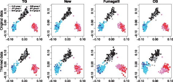
Scatter plots of PC1 (x-axis) versus PC2 (y-axis) in the analysis of the stratified 1000 Genomes data with three discrete Asian populations

Figure 2 shows Q-Q plots for tests of association calculated at each SNP. Because there is no true association, the extent to which these plots track the 45° line is a measure of how well the PCs calculated by each method control for population stratification. For CG, the departure of the observed p-values from the global null hypothesis of no association may be too subtle to be seen clearly with the original data at $\sim 7\times$; it is much more pronounced with the thinned data at $\sim 4\times$, with genomic control $\lambda =1.17$. New, Fumagalli and TG all led to good control of type I error ($\lambda =1.04$); note that the type I error would be highly inflated ($\lambda =1.22$, Supplementary Fig. S2) without adjusting for any PCs.

Fig. 2.

Q–Q plots of $-{\text{log}}_{10}(\text{observed}$P-values) (y-axis) versus $-{\text{log}}_{10}(\text{expected}$P-values) (x-axis) in the analysis of the stratified 1000 Genomes data with three discrete Asian populations. The solid black line represents the reference line of global null hypothesis of no association. The dashed curves represent a 95% point-wise confidence band

3.2 Inference on an admixed population from 1000 Genomes

Applying QC filters to the admixed population data resulted in 43 503 SNPs exome wide; LD pruning reduced this number to 34 563 SNPs. After thinning the depth of WGS to $\sim 4\times$, 24 939 SNPs remained, of which 21 215 SNPs were available for calculating PCs after LD pruning. We calculated PCs using New, Fumagalli, CG and TG and compared the estimated proportions of African ancestry from each method with that calculated using TG; these results are shown in Figure 3 (for values in [0.55, 0.9]) and Supplementary Figure S3 (for all values). The estimates using New agreed closely with those using TG for either the original or the thinned data. By contrast, the estimates using Fumagalli and CG were biased; this bias was more severe with the thinned data. We also quantified the deviation from the values obtained using TG by calculating the sum of squared differences (SS) between estimates obtained using each method and those obtained by TG. New had the lowest value of SS, which was very close to zero and much lower than those of Fumagalli and CG; values of SS are shown in Figure 3.

Fig. 3.

Agreement between estimated proportions of African ancestry calculated using each method (y-axis) and TG (x-axis) for the analysis of an admixed population from the 1000 Genomes Project. SS is the sum of squared difference between the displayed method and TG. The axes are restricted to [0.55, 0.9] to show more detail for the majority of samples; plots showing the full range [0, 1] can be found in Supplementary Figure S3

3.3 Simulation studies

For calculating PCs in each replicate, we considered a random set of 5K, a random set of 50K and all 100K SNPs, as well as a common practice of using 10K AIMs. We applied the New, Fumagalli, CG and TG methods. Note that TG now refers to the PCA method based on true genotypes.

We first verified the type I error rate for association testing in the presence of population stratification in a wider range of scenarios than seen in the stratified (3-subpopulation) 1000 Genomes dataset. For each simulation replicate, we tested for association using each of the 100K SNPs and using the score test for logistic regression. We used 100 data replicates, so that the type I error results displayed in Table 1 are based on 10 M tests. In all scenarios, New and Fumagalli had similar type I error rates as TG (though TG had slightly inflated size when the sample size was 300). The performance of CG was mixed; the type I error rate was sometimes inflated but sometimes zero, depending on the scenario. Note that the scenarios in the second and fourth rows under ‘5K SNPs’ mostly resembled the first 1000 Genomes dataset and had similar results.

Table 1.

Type I error (divided by the nominal significance level of 0.05)

			5K SNPs				50K SNPs				100K SNPs				10K AIMs
n	c0	${\mathrm{ϵ}}_0$	TG	New	F	CG	TG	New	F	CG	TG	New	F	CG	TG	New	F	CG
300	4×	1%	1.09	1.09	1.08	1.24	1.09	1.09	1.07	0	1.09	1.08	1.07	0	1.09	1.09	1.07	1.44
		0.1%	1.09	1.09	1.08	1.21	1.09	1.09	1.07	0	1.09	1.09	1.07	0	1.09	1.09	1.07	1.34
	7×	1%	1.09	1.08	1.08	1.11	1.09	1.08	1.08	1.37	1.08	1.08	1.08	0	1.09	1.08	1.08	1.12
		0.1%	1.09	1.09	1.08	1.10	1.09	1.09	1.08	1.16	1.09	1.08	1.08	1.78	1.09	1.09	1.08	1.10
2000	4×	1%	1.01	1.01	1.02	1.09	1.01	1.01	1.02	0	1.01	1.01	1.03	0	1.01	1.01	1.01	1.12
		0.1%	1.01	1.01	1.02	1.09	1.01	1.01	1.01	0	1.01	1.01	1.01	0	1.01	1.01	1.01	1.11
	7×	1%	1.01	1.01	1.02	1.03	1.01	1.01	1.02	1.05	1.01	1.01	1.01	1.10	1.01	1.01	1.01	1.06
		0.1%	1.01	1.02	1.01	1.03	1.01	1.01	1.01	1.04	1.01	1.01	1.01	1.09	1.01	1.01	1.01	1.05

Note: n is the sample size. c₀ and ${\mathrm{ϵ}}_0$ are the average depth and average error rate in controls. New is the proposed method. F is the Fumagalli method. TG and CG are the PCA methods based on true and called genotypes, respectively. The results are based on 10 M tests.

To get more insights into the mixed performance of CG, we examined the PCs using one replicate of data. In the scatter plots (Fig. 4) of PC1 versus PC2 with 4× average depth and 1% average error rate in controls, we observed that CG caused controls to shift away from cases within each population and the shift became a complete separation when the number of SNPs used for calculating PCs was increased. With 10K AIMs, the shift was less severe but could still be seen. With an average depth of 7× and a much smaller average error rate (0.1%), CG still resulted in a slight shift when calculated using a large number of SNPs (Supplementary Fig. S4). Because we simulated three populations, we expected PC1 and PC2 to capture all genetic variability; thus we expect any information in PC3 and PC4 to be related to differential sequencing. In Figure 5 and Supplementary Figure S5 we see that PC3 calculated using New or TG have no information about subpopulation or case–control status. However, PC3 calculated using CG can be highly informative about the case–control status, indicating a signal arising from differential sequencing quality; this may explain why CG sometimes had zero size. PC1–PC4 calculated using Fumagalli exhibited shrinkage to the origin in the low-depth sequencing group relative to the high-depth group, because the posterior genotype distribution is less informative in the low-depth group. Interestingly, this pattern seemed to have no impact on the type I error.

Fig. 4.

Scatter plots of PC1 (x-axis) versus PC2 (y-axis) in simulation studies with 4× average depth and 1% average error rate in controls. The plots are based on a single replicate dataset generated under the null hypothesis of no association and have data from 150 cases and 150 controls

Fig. 5.

Scatter plots of PC3 (x-axis) versus PC4 (y-axis) in simulation studies with 4× average depth and 1% average error rate in controls. The plots are based on a single replicate dataset generated under the null hypothesis of no association and have data from 150 cases and 150 controls

In Figure 6 we report the effect of PC calculation method on the power to measure a true association; we omit CG because it did not control type I error. New achieved almost the same power as TG in all scenarios. Fumagalli resulted in substantial loss of power when 50K SNPs or 100K SNPs were used for inferring PCs and the controls had 1% average error rate. We found that PC3 by Fumagalli had a large difference in mean between cases and controls in scenarios that Fumagalli lost power (Fig. 7). PC3 seemed to have captured the variance that PC1 and PC2 failed to explain (Figs 4 and 5). Since no difference was expected for PCs other than PC1 and PC2, this PC3 effect was likely the cause of the power loss.

Fig. 6.

Power (y-axis) at the nominal significance level of α = 0.05 over different ORs (x-axis) based on 1000 cases and 1000 controls. The results are based on 1000 tests (10 disease-susceptibility SNPs per replicate and 100 replicates)

Fig. 7.

Mean differences (×100) of top ten PCs between cases and controls. The y-axis represents the absolute difference in mean. The PCs were calculated using 100K SNPs in 100 replicate datasets each having 1000 cases and 1000 controls. The odds ratio $\text{exp}\hspace{0.17em}(\beta )$ was 1.3

4 Discussion

We have presented a robust approach to inferring population structure that is based on analyzing raw sequencing reads directly, without calling genotypes. Our subsampling and read-flipping procedures ensure that the sequencing qualities are matched among all sequencing groups. As a result, the PCs generated from our method do not capture any difference in sequencing qualities, unlike existing methods.

In evaluating our method, we considered discrete populations as well as admixed populations. We have focused on two groups with differential sequencing qualities in the main text, but our method also worked well for studies having three sequencing groups (see Supplementary Text S5 and Fig. S6). In this paper, we have only presented results where one group was sequenced at high depth ($\sim 40\times$) while the another at low depth (7× or 4×). In a situation where both groups had low depth (i.e. cases and controls had 7× and 4×, respectively), our method was still robust to systematic differences in sequencing and efficient in capturing the population structure (see Supplementary Figs S7–S9 and Table S1).

In our simulation studies, we considered different numbers of SNPs for calculating PCs. In practice, the number of SNPs needed to accurately infer population structure and correct for population stratification relies on the degree of population differentiation (Price et al., 2006). Therefore, we recommend using as many SNPs as possible after filtering out rare SNPs, pruning for strong correlations and prioritizing AIMs. If this is computationally prohibitive, we recommend using AIMs and increasing the number of AIMs used until diagnostic plots of PCs stabilize.

In association testing, we used array genotypes in the analysis of 1000 Genomes data (or true genotypes in the simulation studies) for the main effect in the logistic regression. In practice, array genotypes are not always available. More importantly, sequencing studies offer many more SNPs than those on genotyping arrays. We are currently developing methods for association analysis that is based on sequencing reads directly (for both the main effect and the ancestry correction), without using array genotypes or calling genotypes. In this work, we used array genotypes to ensure that the effects we reported were due to the way PCs were calculated, rather than (possibly differential) error in the genotype used to fit the risk model.

Our approach was based on some simplifying assumptions. First, we assumed that the error rate at a SNP was the same across samples in a sequencing group, which was directly estimated from the read count data without using any information on phred scores and mapping scores. In the analysis of the 1000 Genomes data, we filtered out reads with mapping scores < 30 and removed bases with phred scores < 20, so that the assumption of uniform error rate is reasonable. Second, we assumed that errors were symmetric, i.e. that the probability of a read for the major allele being mis-called as the minor allele was the same as the probability of the minor allele being mis-called as the major allele.

The software program implementing our method is readily scalable to genome-wide analysis. For example, with 1000 cases at $\sim 39.5\times$ and 1000 controls at $\sim 4\times$, it took ∼7 h on a single thread of an Intel Xeon X5650 machine with 2.67 GHz to calculate the PCs based on 100K SNPs and 100 repeats of the subsampling and read flipping procedures. When only 10K AIMs were used, it took only ∼0.7 h. In general, the computation increases linearly with the number of individuals, the number of SNPs and the read depth. Additionally, our program allows parallelization of the multiple repeats of subsampling and read flipping on multiple machines.

Our method requires the read count data at each SNP, which is readily available in the raw variant call format (VCF) files that are generated from GATK (with field name ‘AD’) or SAMtools (with field name ‘DP4’). Unfortunately, many publicly available VCF files have been trimmed so that the read count information is lost (e.g. the VCF files on the 1000 Genomes website). We have shown here, and in other settings (Hu et al., 2016), that the information in this single field can allow for adjustment of differential sequencing quality. For this reason, we advocate that this information be kept in future VCF files, so that we do not need the raw BAM files. Alternatively, we provide software to extract the read count data from raw BAM files.

Funding

This research was supported by the National Institutes of Health awards R01GM116065 (Hu).

Disclaimer

The findings and conclusions in this report are those of the authors and do not necessarily represent the official position of the Centers for Disease Control and Prevention.

Conflict of Interest: none declared.

References

- Cavalli-Sforza L. et al. (1993) Demic expansions and human evolution. Science, 259, 639–646. [DOI] [PubMed] [Google Scholar]
- DePristo M.A. et al. (2011) A framework for variation discovery and genotyping using next-generation DNA sequencing data. Nat. Genet., 43, 491–498. [DOI] [PMC free article] [PubMed] [Google Scholar]
- Fumagalli M. et al. (2013) Quantifying population genetic differentiation from next-generation sequencing data. Genetics, 195, 979–992. [DOI] [PMC free article] [PubMed] [Google Scholar]
- Hellmann I. et al. (2008) Population genetic analysis of shotgun assemblies of genomic sequences from multiple individuals. Genome Res., 18, 1020–1029. [DOI] [PMC free article] [PubMed] [Google Scholar]
- Hu Y.J. et al. (2016) Testing rare-variant association without calling genotypes allows for systematic differences in sequencing between cases and controls. PLoS Genet., 12, e1006040. [DOI] [PMC free article] [PubMed] [Google Scholar]
- Johnson P.L.F., Slatkin M. (2008) Accounting for bias from sequencing error in population genetic estimates. Mol. Biol. Evol., 25, 199.. [DOI] [PubMed] [Google Scholar]
- Junemann S. et al. (2013) Updating benchtop sequencing performance comparison. Nat. Biotechnol., 31, 294–296. [DOI] [PubMed] [Google Scholar]
- Kim S.Y. et al. (2011) Estimation of allele frequency and association mapping using next-generation sequencing data. BMC Bioinformatics, 12, 231.. [DOI] [PMC free article] [PubMed] [Google Scholar]
- Li H. et al. (2009) The Sequence Alignment/Map format and SAMtools. Bioinformatics, 25, 2078–2079. [DOI] [PMC free article] [PubMed] [Google Scholar]
- Luo Y. et al. (2017) Exploring the genetic architecture of inflammatory bowel disease by whole-genome sequencing identifies association at ADCY7. Nat. Genet., 49, 186–192. [DOI] [PMC free article] [PubMed] [Google Scholar]
- Ma J. et al. (2012) Principal components analysis of population admixture. PLoS ONE, 7, 1–12. [DOI] [PMC free article] [PubMed] [Google Scholar]
- Martin E.R. et al. (2010) SeqEM: an adaptive genotype-calling approach for next-generation sequencing studies. Bioinformatics, 26, 2803–2810. [DOI] [PMC free article] [PubMed] [Google Scholar]
- Menozzi P. et al. (1978) Synthetic maps of human gene frequencies in Europeans. Science, 201, 786–792. [DOI] [PubMed] [Google Scholar]
- Nielsen R. et al. (2011) Genotype and SNP calling from next-generation sequencing data. Nat. Rev. Genet., 12, 443–451. [DOI] [PMC free article] [PubMed] [Google Scholar]
- Pardo-Seco J. et al. (2014) Evaluating the accuracy of AIM panels at quantifying genome ancestry. BMC Genomics, 15, 543.. [DOI] [PMC free article] [PubMed] [Google Scholar]
- Price A.L. et al. (2006) Principal components analysis corrects for stratification in genome-wide association studies. Nat. Genet., 38, 904–909. [DOI] [PubMed] [Google Scholar]
- Purcell S. et al. (2007) Plink: a tool set for whole-genome association and population-based linkage analyses. Am. J. Hum. Genet., 81, 559–575. [DOI] [PMC free article] [PubMed] [Google Scholar]
- Reich D. et al. (2008) Principal component analysis of genetic data. Nat. Genet., 40, 491–492. [DOI] [PubMed] [Google Scholar]
- The 1000 Genomes Project Consortium. (2010) A map of human genome variation from population-scale sequencing. Nature, 467, 1061–1073. [DOI] [PMC free article] [PubMed] [Google Scholar]
- The UK10K Consortium. (2015) The UK10K project identifies rare variants in health and disease. Nature, 526, 82–90. [DOI] [PMC free article] [PubMed] [Google Scholar]
- Tian C. et al. (2008) Analysis of East Asia genetic substructure using genome-wide SNP arrays. PLoS ONE, 3, e3862. [DOI] [PMC free article] [PubMed] [Google Scholar]
- Wang C. et al. (2014) Ancestry estimation and control of population stratification for sequence-based association studies. Nat. Genet., 46, 409–415. [DOI] [PMC free article] [PubMed] [Google Scholar]
- Zoledziewska M. et al. (2015) Height-reducing variants and selection for short stature in Sardinia. Nat. Genet., 47, 1352–1356. [DOI] [PMC free article] [PubMed] [Google Scholar]
Associated Data
This section collects any data citations, data availability statements, or supplementary materials included in this article.