Segmentation of vessel structures from photoacoustic images with reliability assessment

Abstract

Photoacoustic imaging enables the imaging of soft biological tissue with combined optical contrast and ultrasound resolution. One of the targets of interest is tissue vasculature. However, the photoacoustic images may not directly provide the information on, for example, vasculature structure. Therefore, the images are improved by reducing noise and artefacts, and processed for better visualisation of the target of interest. In this work, we present a new segmentation method of photoacoustic images that also straightforwardly produces assessments of its reliability. The segmentation depends on parameters which have a natural tendency to increase the reliability as the parameter values monotonically change. The reliability is assessed by counting classifications of image voxels with different parameter values. The resulting segmentation with reliability offers new ways and tools to analyse photoacoustic images and new possibilities for utilising them as anatomical priors in further computations. Our MATLAB implementation of the method is available as an open-source software package [P. Raumonen, Matlab, 2018].

1. Introduction

Photoacoustic tomography (PAT) is an imaging modality based on the photoacoustic effect that is generated through the absorption of an externally introduced light pulse. The method combines optical contrast provided by distinctive absorption spectra by different chromophores with high spatial resolution of ultrasound. The chromophores of interest are, for example, haemoglobin, melanin and various contrast agents. In soft biological tissue, the ultrasonic waves carry this optical information to the surface of tissue with minimal scattering, thus retaining accurate spatial information as well. PAT can be used to provide images of soft biological tissues with high spatial resolution. It has successfully been applied to the visualisation of different structures in biological tissues, such as human blood vessels, microvasculature of tumours, and the cerebral cortex in small animals. For more information about PAT, see e.g. the reviews [1–8] and the references therein.

In the inverse problem of PAT, the initial pressure distribution caused the by the light absorption is estimated from the pressure waves measured on the surface of the tissue. Various methods for the solution of this problem have been developed including analytical inversion methods such as backprojection algorithms [9–11] and eigenfunction expansion [12, 13], time-reversal [14–18], regularized least squares [19–26] and Bayesian approach [27, 28]. If the object is fully surrounded by detectors on a closed surface, the inverse problems of PAT is not ill-posed and can provide good quality reconstructions of the whole three dimensional (3D) volume. However, in practice, such an experimental setting cannot typically be constructed and one is restricted to perform the measurements from limited directions. It has been shown that, in limited-view measurement geometries, the target regions that are enclosed by the detection surface can be reconstructed accurately [29]. Those inclusions within the object, that are not enclosed by the detection surface, suffer from distortions apart from those inclusion boundaries whose normals intersect the detection surface [29].

In order to provide meaningful information of the target of interest, the estimated initial pressure may be further processed using methods of image processing for example by reducing limited-view artefacts and noise, correcting image intensity by light attenuation model, segmenting tissue types or exogenous absorbers etc. Furthermore, in quantitative PAT, one takes the estimated initial pressure as data and aims at reconstructing the distributions of the light absorbing molecules [30]. This is an ill-posed problem which is severely affected by the solution method of the acoustic inverse problem and the noise and artefacts in the reconstructed initial pressure [31].

Image segmentation has been utilised in PAT for example in finding the skin surface [32], finding regions with different speed of sound [33], determining vessel separations to guide surgeries [34] and simplifying the reconstruction geometry for quantitative PAT in a simple phantom measurement setup [35, 36]. In addition, an automatic segmentation designed to distinguish blood vessels called vessel filtering [37] has been applied for photoacoustic images in [38]. The method has been further improved by skeletonization algorithm developed for vessel architectural analysis [39]. The distortions in the photoacoustic images and noise make filtering and segmentation process challenging, and thus further development of automated methods for segmentation are required.

Conventional filtering and segmentation methods produce either a single processed and filtered image or a single segmentation of the image into vessels and other parts. However, there can be considerable problems with these approaches. For example, the results are generated by some kind of optimisation of the input parameters or even by a priori fixed parameters which results in a classification where every point is either vessel or non-vessel. Thus, some voxels are easily classified totally wrong as there are no middle ground or gradation. On the other hand, if the image is not classified into two classes but only improved and filtered for visual study, the intensities after the processing are not directly indicative of presence of vessels. Furthermore, the results may be sensitive to small changes in the parameter values controlling the segmentation and this sensitivity is quite rarely explicitly estimated or acknowledged. There are also the questions how appropriate the selected optimisation criteria are and what would happen if they were changed. Another and related problem is that we usually do not have any quantitative (or even qualitative) measure how reliable the segmentation result is, locally or globally.

In this paper, vessel segmentation is approached in a probabilistic framework. We use a classification procedure whose parameters have the property (at least approximately) that when the parameter values are monotonically changed (e.g. decreased), new additional image voxels are classified as vessels but with less reliability. Instead of trying to optimise the parameters of the classification procedure, we repeat the procedure many times by uniformly sweeping over the parameter space of the procedure. Then we count the classifications (vessel, non-vessel) for every voxels and this count then gives the reliability estimation for each voxel. Thus, the result of the segmentation process is an image where the intensity is replaced with confidence or reliability value of how likely the voxel is from a vessel.

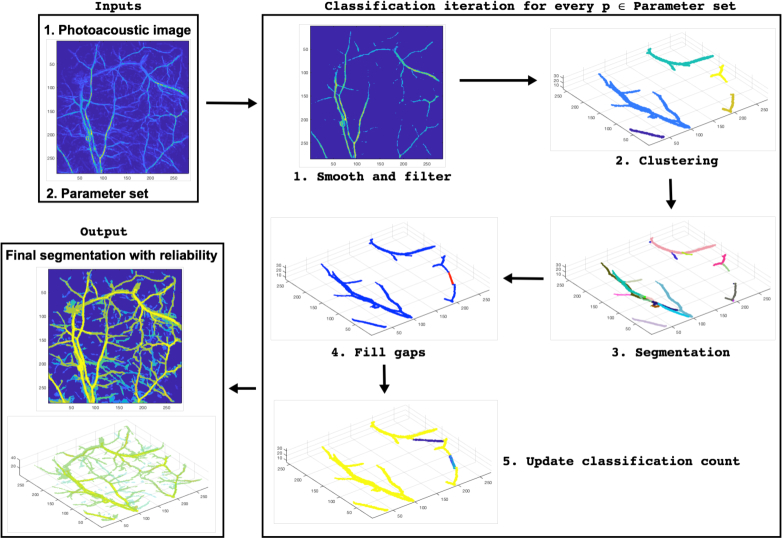
The classification procedure has four main steps: 1) smoothing and filtering the data, 2) clustering, 3) vessel-segmentation of the clusters, and 4) filling gaps in the segmented data. The procedure utilises volumetric data (point clouds) which allows for efficient processing and visualisation of the data. Similar approach has been previously utilised in segmenting tree branches from lidar data [40].

The content of the paper is as follows. In Section 2, we present an overview and details of the classification procedure and how to apply it for reliability estimation. In Section 3, we present the material we are using for testing and validating the method. Both numerical simulations with synthetic data and real experimental photoacoustic images are used to evaluate the performance of the method. In Section 4, we use the synthetic data for sensitivity analysis. Then, in Section 5, we apply the method to real photoacoustic images and do performance estimation with visual inspection. Finally, in Section 6, we discus the results and future possibilities and present some conclusions.

2. Segmentation method

2.1. Overview of the method

The method for segmentation of vessel structures with reliability consists of a classification procedure that is repeated using a large number of input parameters which determine the probability of each voxel of a given image to be classified as a vessel. The parameters of the procedure are such that when we use extreme values on one end of the spectrum, the voxels classified as vessels have very high reliability. When the parameter values approach the other end of the spectrum, new additional voxels are classified as vessels but with less reliability. The classification procedure has four main steps: 1) smoothing and filtering the data, 2) clustering, 3) segmentation of the clusters into vessels, and 4) filling gaps in the vessel-segmented data. A flowchart of the methodology is shown in Fig. 1.

Fig. 1.

A flowchart of the segmentation methodology.

In the first step, 1) smoothing and filtering the data, smoothing is performed by the convolution of the image with a small ball-supported kernel. Then, a simple threshold-filtering is applied to the smoothed data. We call this neighbourhood smoothing and filtering. Notice, that with high thresholds for filtering the voxels are classified as vessels with high reliability, and decreasing the threshold increases the number of voxels classified as vessel but with less reliability.

In the second step, 2) clustering, the data is segmented into connected vessel structures or networks based on region growing. The clustering has a given minimum intensity value as a starting point of a cluster and a given minimum relative intensity value of the neighbouring points to be included in the cluster. Note, that a large starting intensity and a large neighbour intensity leads the voxels to be classified as vessel with a high reliability, and decreasing these values increases the number of voxels classified as vessel but with less reliability.

In the third step, 3) segmentation of the clusters into vessels, each vessel network is segmented into smaller segments without bifurcations. In other words, the segments correspond approximately to individual vessels. This step has no parameters that are varied in the classification procedure.

In the fourth step, 4) filling gaps in the vessel-segmented data, potential tips (breaks) of the segmented vessels are determined and some gaps between these tips are filled. In the approach, two vessel tips from different clusters are combined if the gap between them is shorter than a given maximum length and if the angle between the tip directions is less than a given maximum angle. Similarly to the filtering and clustering thresholds, if we have a small length and a small angle we can close a gap with higher reliability and if we increase the length and the angle we can close additional gaps but with less reliability.

2.2. Neighbourhood smoothing and filtering

A photoacoustic image has noise that makes the data discontinuous. To smooth the data and filter out less reliable background values we present a very simple smoothing and filtering method. The idea is to average the intensity values over a small ball-like neighbourhood to get smoother data. The neighbourhood average also indicates in direct and simple way if the voxel is part of a structure: voxels that are part of a structure are more likely to have a higher average neighbourhood intensity than ’noisy voxels’ or ’background voxels’. This smoothed data, where the intensity of each voxel is replaced with the average intensity of its neighbourhood voxels, can then be filtered simply by a given threshold: if the intensity of a voxel is lower than the threshold value, then its value is set to zero. An example of images with different filtering thresholds can be seen in Fig. 2. The details of the utilised photoacoustic image are described later in Section 3.1.

Fig. 2.

Comparison of smoothed data with different filtering thresholds. The threshold is decreased from left to right and the rightmost image is the original non-smoothed and unfiltered data. The images are maximum-intensity projections.

The smoothing (averaging) can be implemented as a convolution of 3D-arrays where the data array is convolved with a small binary array whose non-zero elements are all ones and form a ball-like support. In this work, we used 3 voxels as the diameter of the ball. Note that the size of the ball could be another parameter to be varied in the reliability estimation. Although, it did not play a significant role in our simulations, the parameter may have more value in other cases, e.g. if the diameters of the vessels are large in terms of voxels.

The threshold used in the filtering of the smoothed data is one of the parameters to be varied in the reliability assessment of the proposed segmentation method. We select a set of parameter values for the threshold that corresponds to an interesting range for the segmentation. For a given smoothing, we can compute the relative proportion of voxels passing the filtering with different threshold values (Fig. 3 shows a typical result). As it can be seen, the curve of proportion passing the filtering behaves similar to 1/x-function: there is a rapid decrease in the proportion with small thresholds, but with larger thresholds, the decrease is very slow. This suggest that the threshold values used for the filtering could be selected quantitatively. In this work, we use the following approach based on the derivative values of the proportion curve: the lower threshold bound is set to the intensity value where the derivative of the proportions curve is approximately −1 and the upper threshold bound is set to the intensity value where the derivative is approximately −0.15. This choice covers the most of the ’bend’ of the proportions curve which can be regarded as the interval of most interest. Then, we select these thresholds and some numbers between the bounds so that the corresponding proportions are uniformly distributed.

Fig. 3.

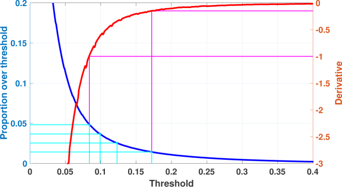
Selecting the values for the filtering threshold. The blue curve shows the proportion of the voxels passing the filtering as a function of the intensity values. The red curve is the estimated derivative of the blue curve. The magenta lines show how to determine the limit threshold values by the given derivative values of −1 and −0.15. The cyan lines show the uniformly distributed proportion values and define the filtering threshold intensities.

It should be noted that the intensity of the photoacoustic image may vary depending on the distance to the ultrasound sensor, especially if one is examining large imaging volumes using a limited-view set-up. In those cases, one may need to apply a spatially varying threshold to distinguish all the features in the images or apply an intensity correction based on light attenuation model to the image before filtering.

2.3. Clustering

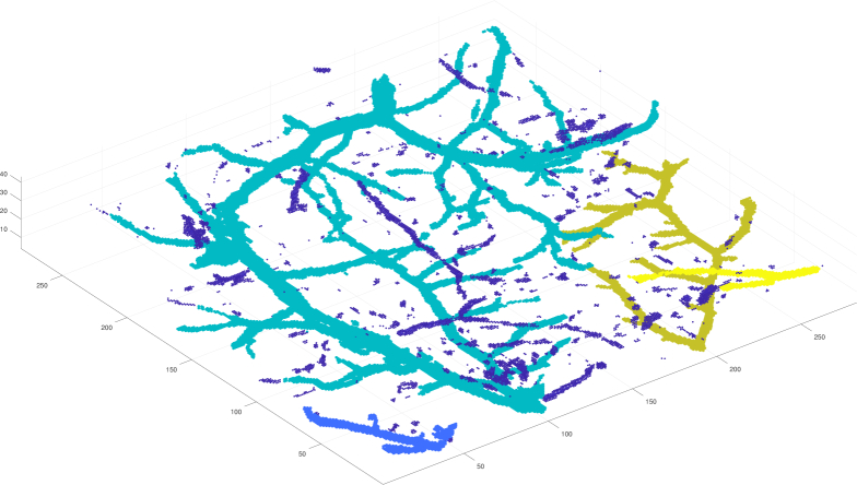
After the filtering, most of the voxels of the image are zero, and therefore it makes sense to represent the non-zero data as a point cloud (subset of ℝ³), where the coordinates of the points are their array indices and the intensity value is assigned to each point. Point clouds are also better for visualisation and they inherit the neighbourhood structure from the 3D-array. See an example of a point cloud in Fig. 4.

Fig. 4.

Clustering point cloud based on intensity. There are four clusters shown with different colours. The dark blue points scattered around are the points not assigned to any cluster because of too low intensity values.

Next we separate likely vessel structures from the point cloud as clusters. We use simple intensity-based region growing to form the clusters with the idea that a point that has relatively high intensity and is connected to a high-intensity point is likely from the same cluster. The starting point of the first cluster is the point with the highest intensity, and the possible following starting point is always the highest intensity point not yet assigned to any cluster. Then a neighbour point is added to a growing cluster if its intensity is high enough compared to the intensity of the starting point. The minimum acceptable size of the cluster can be controlled and in this paper it is fixed to 20 points. Usually a resulting cluster is a connected network of many small and large vessels as seen in Fig. 4.

The clustering procedure contains two parameter that are varied in the reliability assessment: the minimum acceptable intensity for a starting point and the minimum relative intensity (compared to the minimum acceptable intensity) of an acceptable neighbour. We propose that the minimum acceptable intensities for a starting point are determined by a user given uniformly distributed proportions. That is, a given proportion value, say 90%, defines the intensity value below which 90% of the non-zero intensities are. Fig. 5 shows an example of this parameter value determination. The values of the the minimum relative intensity of the acceptable neighbour are uniformly distributed and given by the user.

Fig. 5.

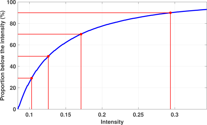
Selecting the values for the minimum intensity of the region growing starting points. The blue curve shows the proportion of the points below the given intensity value. The red dots on the curve correspond to the user given uniformly distributed proportion values, here [30 50 70 90]%, and define the minimum intensities.

2.4. Vessel-segmentation of the clusters

The clusters usually correspond to a connected network of many different size vessels where smaller vessels branches off from bigger vessels. In order to locate the tips of the vessels so that possible gaps/breaks in the vessel structure can be filled, we next segment the clusters into vessels. For this vessel-segmentation we use the method presented in [40] which was first developed for branch-segmentation of LiDAR point clouds from trees. The idea of the method is to use small connected subsets (’sets’) of the point cloud and use their neighbour-relation for locating bifurcation points in the vessel structure: Starting from some collection of sets (’base’), we select a collection of sets consisting of few layers of neighbouring sets (’section’) and check the connectedness of this section. We proceed iteratively by moving the section one layer of neighbours forward and at each step check the connectivity of the section. If there is a bifurcation, then the section becomes disconnected at some point and all or all but one of the components of the section start a new vessel and in most cases the biggest component continues the current segment. We segment each cluster twice: first segmentation with bigger subsets and with heuristic base determines the base of the second and final segmentation which is processed with smaller subsets to achieve more accurate segmentation.

First, we partition the clusters into small connected subsets, whose diameter varies between 3 and 6 units for the first segmentation and between 1.5 and 3 units for the second segmentation, using random Voronoi tessellations (Fig. 6 shows an example of the tessellation). The tessellation method is presented in [40] and it also defines naturally possible neighbours for every set. Next, we select for each cluster the base for the first segmentation: We select the set that has the least number of neighbours as the base because it is likely from a vessel tip. Then we start the vessel-segmentation from these bases and use the following rule when there is a bifurcation point: always continue the current segment with the section component that has the most sets. The vessel tips of the first segmentation provide a reliable way to select the bases for the second segmentation: We select the widest tip to be the base and we estimate the widths by the number of the sets in the three set-layers forming the tip. For the second segmentation we use the different rule when there is a bifurcation point: continue the current segment with the section component that has the most sets and has at least 1.5 times the number of sets compared to the second largest section component. Fig. 6 shows an example of the final vessel-segmentation.

Fig. 6.

Segmentation of the clusters based on tessellations. Left: Tessellation of the clusters into connected subsets. Right: Vessel-segmentation.

2.5. Closing gaps in the data

The segments obtained from the vessel-segmentation are connected regions of relatively high intensity points. However, due to limitations of sensor configurations, there can be gaps in the segmentations or other limited-view artefacts. For example, parts of some vessels, that are behind other vessels when seen from sensors, may not be visible in photoacoustic images. The next step in the classification procedure is to find likely gaps and close them by adding new points.

First, we select all the vessel tips from the vessel-segmentation and estimate their direction. The next step is to find suitable tip pairs from different clusters to be connected by filling the gap between them. The idea is to use pairs whose tips are close to each other and whose directions are almost parallel. The closer and the more parallel the pairs are, the more confident we can be that they should be connected. The gap between a suitable pair is closed by joining the points in the tips with lines and then points on those lines define a small set of new unique vessel points with integer coordinates.

We have two parameters that control the search of tip pairs and whose values are varied for the reliability assessment: the maximum distance between pairs and the maximum angle between the direction lines of the pairs. For the reliability assessment, the user defines uniformly distributed set of distance and angle values. If a gap is closed by with the smallest distance and angle values, it is also closed by all the other distance and angle values, and thus gets counted more times and is estimated to be more reliably closed than gaps with larger distances or angles.

2.6. Reliability assessment

The classification procedure explained above gives the voxels that are classified as vessels. The procedure has five parameters that control the outcome, and thus changing the values of these parameters may result in different classifications. Instead of trying to find the optimal values for these parameters, we define quite broad ranges of values for each parameter and then apply the classification procedure with every possible combination of the parameter values. Then, we count the relative frequency of vessel classification for every voxel and this relative frequency is our quantified reliability for vessel classification.

The five parameters and their potential values used for iterative classification are:

• Fil = Threshold intensity for filtering. Determined from the user given boundary derivative values of the proportions of voxels passing the filtering. Using derivative values of approximately −1 and −0.05 could result in thresholds such as [0.07, 0.09, 0.12, 0.27].

• Sta = The minimum intensity for starting points of clusters. Determined from the user given proportions that specify the proportion of points below the starting intensity. Reasonable values for the proportions could be e.g. [90, 70, 50, 30]%, which could result in minimum intensities such as [0.60, 0.45, 0.38, 0.32]

• Nei = Relative intensity of the acceptable neighbour for neighbourhood growing. Reasonable values could be e.g. [0.6, 0.5, 0.4, 0.3].

• Dis = The maximum distance between the vessel tips that can be combined. Reasonable values could be e.g. [5, 10, 15, 20] voxels.

• Ang = The maximum angle between directions of the vessel tips that can be combined. Reasonable values could be e.g. [20, 30, 40, 50] degrees.

There are many things to observe here. First, with this selection of parameter values there are 5⁴ or 625 different parameter combinations that are used for classification procedure. However, this does not mean that e.g. the smoothing and filtering must be done 625 times but only 4 times and each smoothed and filtered data is then clustered and vessel-segmented 16 times since these steps are done in series. Furthermore, the gap filling for the vessel-segmented data can be done only once and the classification count is updated based on the distances and angles. Second, the values of these parameters could be selected differently, and in fact we will make a sensitivity analysis for the choice of the values in Section 4.2. Third, there could be additional parameters in our procedure such as the diameter of the ball used in the smoothing (now fixed to three voxels) or the minimum acceptable component size for the clustering (now fixed to 20 voxels). However, adding parameters, particularly ones that are not very important, only increases the computation time without necessarily giving much interesting or useful information. Fourth, the number of values each parameter has may affect the solution, i.e. the quantified reliability. This is basically about weighting different aspects of the classification, e.g. filtering over the clustering. However, this is closely related to parameter sensitivity and parameter selection in general. In this paper we keep the number of values for each parameter the same, i.e. equal weights, and do not study this aspect of parameter selection any further. Finally, the reliability assessment procedure based on iterative classification is not limited to the four-step classification procedure proposed in this work but it can be applied to other segmentation procedures, particularly if their parameters have approximately monotonic tendency in the reliability. We have implemented the segmentation method in MATLAB following the details described in the above subsections and it is available as an open-source software package [ Code 1, [41]].

3. Materials

3.1. Real data

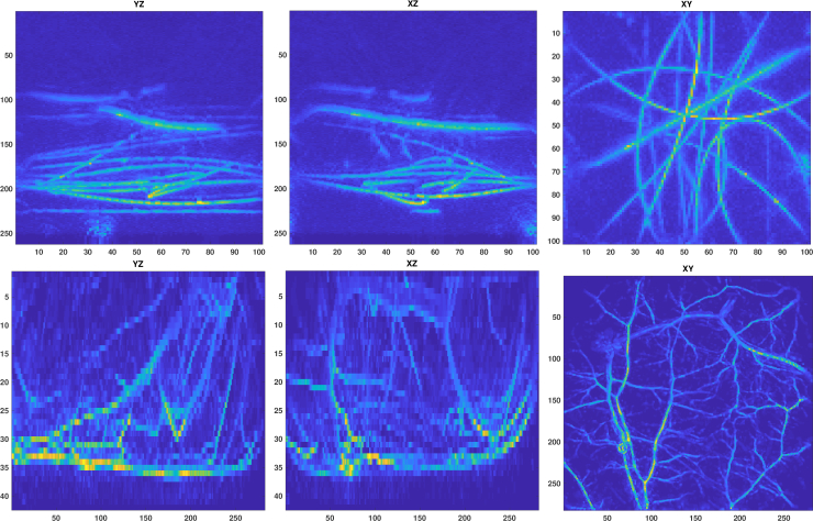
Two 3D photoacoustic images were used to test the vessel segmentation with reliability procedure. The images were obtained from phantom and in vivo photoacoustic experiments performed with a photoacoustic measurement system of the Photoacoustic Imaging Group of University College London with a planar Fabry-Pérot sensor head [42]. The phantom experiment was performed with a tissue mimicking phantom design to present a network of blood vessels [42]. It comprised an arrangement of polymer tubes filled with blood which were immersed in a turbid liquid. The in vivo data set represents skin vasculature and subcutaneous anatomy near the right flank of a nude mouse [43]. For more information on the experiments and the photoacoustic imaging system, see e.g. [42, 43]. The photoacoustic images were reconstructed from the measured experimental data using a time-reversal method implemented with the k-Wave MATLAB toolbox [44]. The maximum intensity projections of the photoacoustic images are shown in Fig. 7.

Fig. 7.

Two 3D-photoacoustic images from phantom (top row) and in vivo (bottom row) experiments. Images from left to right are maximum intensity projections into x-, y- and z-directions.

3.2. Synthetic data

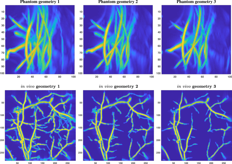
The synthetic data was generated from the photoacoustic images obtained with the real experiments. The synthetic photoacoustic images were generated to perform assessments of the method and quantitative comparisons with known true values. The parameter sensitivity was tested and complete quantitative assessment was performed with these synthetic photoacoustic images.

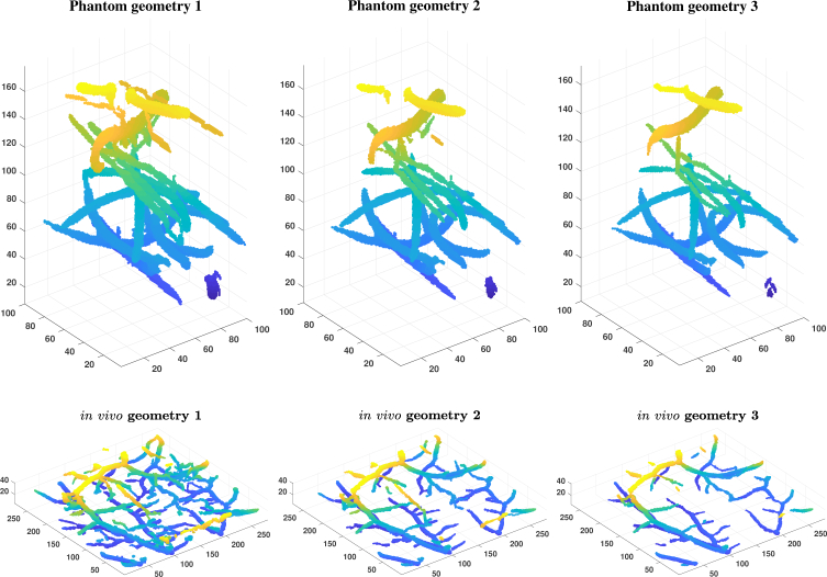
We generated six different synthetic images, three images from the phantom experiment which we will refer as phantom geometries 1, 2, and 3 and three images from the in vivo vasculature experiment which we will refer as in vivo geometries 1, 2 and 3, as follows. First, we applied modified version of our segmentation procedure with a small set of parameters. Instead of using the our neighbourhood smoothing and filtering, we used the vessel filtering by Oruganti et al. [38] where the Gaussians had [0.5, 1.0, 1.5, 2.0, 2.5, 3.0] voxels for standard deviation and then applied threshold filtering with 0.05, 0.1 and 0.15 as the thresholds. After the vessel filtering, we applied the last three steps of our classification procedure with the following parameters: Sta = 0.2, Nei = 0.3, Dis = 25 voxels and Ang = 30 degrees. The resulting segmentations were then turned into binary models of vessel geometries by changing every non-zero voxel into one and this binary model formed our vessel geometry. The prevalence or the relative portion of the vessel points are 1.21%, 0.80% and 0.59% in the phantom geometries 1, 2 and 3 and 2.21%, 1.31% and 0.93% in the in vivo geometries 1, 2 and 3. The synthetic vessel geometries are shown in Fig. 8.

Fig. 8.

Vessel geometries used for production of synthetic photoacoustic images. The colour of the images denotes the z-coordinate.

After the geometries were generated, we simulated photoacoustic measurements and reconstructed photoacoustic images in the simulated geometries using the k-Wave toolbox as follows. Each voxel was given a side length 0.1 mm. The geometries phantom 1, 2 and 3 consisted of 101, 101 and 262 voxels into x- y- and z-directions, respectively, and the size of the geometry was 10.1 mm × 10.1 mm × 26.2 mm. The in vivo geometries 1, 2 and 3 consisted of 282, 282 and 42 voxels into x- y- and z-directions, respectively, and the size of the geometry was 28.2 mm × 28.2 mm × 4.2 mm. The vessels were given an initial pressure of 10 and the background initial pressure was set to zero. The speed of sound was set c = 1500 m/s and the medium was assumed to acoustically be non-attenuating. The sensors were modelled to locate on each grid coordinate on the boundary of the geometry. This corresponds to a somewhat idealistic measurement geometry in which one is able to capture the photoacoustic time series on each side of the target with a large number of detectors. The propagation of pressure wave was simulated using a k-space method implemented with the k-Wave toolbox. Normally distributed random noise with standard deviation corresponding to 1% of the peak amplitude of the simulated pressure signal was added to the data to simulate noise in measurement data. Then, the initial pressure was reconstructed using a time-reversal method implemented with the k-Wave toolbox. In the reconstruction, the same voxel discretisation was used. This corresponds to an inverse crime which can lead to unrealistic good reconstructions if one is developing inverse problem solution methods. However, in this case, the purpose was to produce ’idealistic’ photoacoustic image that could be used to investigate the performance of the segmentation procedure and using the same discretisation enabled that.

The simulated photoacoustic images are shown in Fig. 9. In the synthetic photoacoustic images the relative portion of non-zero intensity points is about 56% for phantom geometries 1, 2 and 3 and about 65% for in vivo geometries 1, 2 and 3. Notice that there are tens of times more non-zero intensity points in the simulated photoacoustic images than there are vessel points in the synthetic vessel geometries. It should be also noted that a more realistic photoacoustic simulation would include simulating light propagation and absorption in a heterogeneous target. In this work, that was not considered with simulations since we had real experimental data to test the proposed methodology.

Fig. 9.

The synthetic photoacoustic images reconstructed from the vessel geometries shown in Fig. 8. The images are maximum intensity projections into z-direction.

4. Numerical experiments

4.1. Quantitative analysis

We use the synthetic data presented in Section 3.2 to quantitatively analyse the sensitivity of the methodology on selected parameter values. We use the following standard measures to quantify the segmentation success and errors:

• True positive rate (a.k.a. recal or probability of detection), i.e. the number of correctly classified vessel points divided by the number of vessel points.

• False positive rate (a.k.a. fall-out or probability of false alarm), the number of points incorrectly classified as vessels divided by the number of non-vessel points.

• True negative rate (a.k.a. specificity), the number of correctly classified non-vessel points divided by the number of non-vessel points.

• False negative rate (a.k.a. miss rate), the number of points incorrectly classified as non-vessels divided by the number of vessel points.

• Accuracy, the sum of correctly classified vessel and non-vessel points divided by the number of all points.

Because our segmentation comes with the reliability, the above measures can be given as functions of the minimum reliability level such that the measures are computed for all the voxels with equal or higher than a given reliability. Moreover, the results can be summarized compactly as graphs of the functions.

4.2. Sensitivity analysis

A useful segmentation method should be robust, which in our case means that the resulting classification reliability of voxels should not be too sensitive to the choices of the parameter values used for the segmentation. In other words, if we change the parameter values a little, the results should be almost the same. As described in Section 2.6, the parameter values that can be varied in the segmentation are the threshold intensity for filtering (Fil), the minimum intensity for a starting point of a region growing (Sta), the relative intensity of the acceptable neighbour for neighbourhood growing (Nei), the maximum distance between the vessel tips that can be combined (Dis) and the maximum angle between directions of the vessel tips that can be combined (Ang). In this section, we use the synthetic data to analyse how sensitive our method is for changes in these parameters. We use narrower and wider ranges and cover different parts of the parameter spaces. We use the same number of values for each parameter, i.e. we have the same weights for each parameter.

First, we analyse all five parameters separately to see which parameters are the most sensitive. Then, we analyse all the parameters simultaneously to see if the sensitivities add up. Table 1 shows the values used for the separate analyses.

Table 1.

Parameter values used for the sensitivity analysis. Notice that the values given for Fil and Sta are not the actual intensities but derivative and proportion values that determine the intensities.

Parameter	Range 1	Range 2	Range 3
Fil	[−0.8 −0.07]	[−0.9 −0.03]	[−0.7 −0.05]
Sta	[90 70 50 30]	[93 70.33 47.67 25]	[92 72 52 32]
Nei	[0.6 0.5 0.4 0.3]	[0.65 0.5 0.35 0.2]	[0.65 0.55 0.45 0.35]
Dis	[10 15 20 25]	[5 13.33 21.66 30]	[5 10 15 20]
Ang	[20 30 40 50]	[15 28.33 41.67 55]	[15 25 35 55]

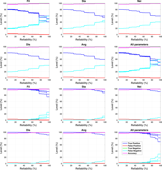
The results for the synthetic photoacoustic data sets, phantom geometry 1 and in vivo geometry 3, evaluated with all parameters are shown in Fig. 10. The results for the other geometries are very similar. If a parameter is sensitive for the choice of the range, then we should see three different lines (one for each range) for each colours (metrics). As we can see, Fil is by far the most sensitive of the parameters but it is not that sensitive either and mostly in the high end of the reliability (over 75%). Sta has very small sensitivity in the highest reliabilities (over 90%). The other parameters are practically indifferent to the choice of these ranges.

Fig. 10.

Parameter sensitivity analysis for phantom geometry 1 (top two rows) and in vivo geometry 3 (bottom two rows). The parameters have three ranges, Range 1 (solid lines), Range 2 (dashdot lines) and Range 3 (dashed lines), which are given in Table 1. The parameters Fil, Sta, Nei, Dis, and Ang are defined in Sec. 2.6. In the horizontal axis “Reliability (%)” indicates the smallest reliability level, and thus all the voxels with a higher reliability are included in the calculated measures. In the vertical axis “Level (%)” indicates the different measures shown in the legend and which are defined in Sec. 4.1. Notice that True Negative (green line) is hardly visible because it has practically the same level as Accuracy (magenta line).

5. Application to photoacoustic images

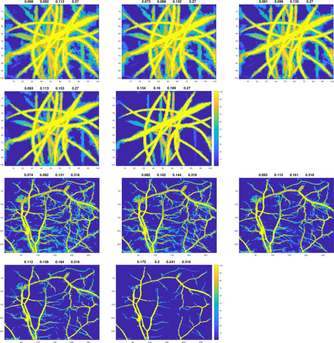
We applied the segmentation to the real photoacoustic images shown in Fig. 7. We tried five different ranges for filtering thresholds Fil which are given in Table 2. For the other parameters we used only the Range 1 from Table 1. The results are shown in Fig. 11.

Table 2.

Testing the segmentation method for real photoacoustic. Derivative values used for determination of the filtering thresholds and the realised thresholds.

Range	Derivative	Fil(phantom)	Fil(in vivo)
1	[−1.35 −0.03]	[.068 .082 .113 .270]	[.074 .092 .131 .316]
2	[−1.05 −0.03]	[.073 .088 .122 .270]	[.082 .102 .144 .316]
3	[−0.75 −0.03]	[.081 .099 .135 .270]	[.093 .115 .161 .316]
4	[−0.45 −0.03]	[.093 .113 .153 .270]	[.112 .138 .184 .316]
5	[−0.15 −0.03]	[.134 .160 .199 .270]	[.172 .200 .241 .316]

Fig. 11.

The real photoacoustic images shown in Fig. 7 segmented with reliability. The images on the two top rows show segmentations from the phantom experiment and the images on the two bottom rows show segmentations from the in vivo experiment. The values above the images are the applied filtering thresholds. The images are maximum reliability projections into z-direction.

These examples show how the segmentation method can segment the main vessels close to 100% reliability and clearly highlight them. On the other hand, the smaller and less clear vessels are segmented distinctly less than 100% reliability but still be clearly highlighted.

These examples show also that the same range of Fil-parameter values do not work for both cases. For the first case, which is the phantom experiment, the fourth range is perhaps the best as it does not include too much but still retains most clear vessel points. For the second case, the in vivo mouse vasculature experiment, the first two ranges (the largest ranges) seems to work best. It should be noted that these two examples are photoacoustic images from very different targets, and thus it cannot be expected that the same thresholds would be suitable for both. Thus, this example can help us to think how the important Fil-parameter values should be selected.

6. Discussion and conclusion

The parameter sensitivity analysis with synthetic photoacoustic images showed that the segmentation procedure is robust to the choice of the parameters (range). It was not surprising that the filtering threshold had the most influence on the reliabilities as it determines how many non-zero points there are for segmentation into vessels.

For phantom geometries 1, 2, and 3 the true positive rate is lower and it is more dependent on the reliability. It particularly has lower rates for high-reliability range. That is, only a little over half of the vessel mimicking voxels were segmented as vessels with very high reliability from the synthetic photoacoustic images simulated for the phantom experiment. On the other hand, the true positive rate for in vivo geometries 1, 2 and 3 are generally very high up to mid reliability range and then decreases down to about 80 − 90% with the highest reliabilities. This indicates that most of the real vessel points were segmented with a high reliability from the synthetic photoacoustic images simulated from the in vivo vasculature experiments.

False positive rate for all geometries was very low with high-reliability and was only a few percentages for low-reliability range. On the other hand, with high-reliability the false positive rate approaches zero, indicating that there are not many points that were incorrectly classified as vessels with high reliability. The true negative rate was close to 100% with any reliability.

The results from the real photoacoustic experiments show that the method is capable of segmenting real photoacoustic images with reliability assessment. However, perhaps the widths and volumes of the vessels were overly estimated, at least for the phantom experiment. This could be due to noise in photoacoustic data, artefacts due to photoacoustic image inversion that can cause image artefacts which can be hard to separate from real vessels and the size of the ball used in the smoothing.

The reliability values obtained as the solution of the vessel segmentation values are more quantitative and comparable than the original photoacoustic intensity images which contain lot of noise, artefacts, and adjustments. However, what reliability values constitute “good” or “high” or “acceptable” values depends on the application and its requirements. In some applications e.g. 75% reliability might be considered “high” but in another application not until 95% reliability is considered “high”. In addition, the reliabilities can further be utilised in quantitative PAT as prior information on tissue structure, and thus will ease the ill-posedness of the estimation problem. For example in Bayesian framework for quantitative PAT, this anatomic information could be combined with tissue specific optical properties [31, 45].

The presented segmentation with reliability assessment, based on repeated classification procedure, is not the definite way to do segmentation with reliability. Neither is the way the reliability was estimated. We can modify the segmentation process or use some other completely different approach and we can modify how the reliability is defined. Thus, segmentation with reliability can be realised in multiple ways and this needs further study.

We only used vessel-segmentation of the clusters as a tool for locating the tips of vessels. But we could also use the segmentation for further analysis and quantification of the vessel structure such as the topology of vessel networks and the geometry of vessels (lengths, diameters and volumes).

We used synthetic photoacoustic images for accurate quantitative analysis of the results. The further step in this regard could be to analyse how well the reconstruction was locally instead of global count of correct and incorrect classifications. This kind of local analysis requires different metrics that might be application specific. We could also analyse how well gaps in the data were closed and how to recognise artefacts. However, the gaps and the artefacts in photoacoustic images are different depending on the measurement procedure, for example number and location of ultrasound sensors, their frequency response, method used for reconstructing the photoacoustic images, etc. Thus, the further analysis and the selection of parameter ranges for the segmentation are most likely dependent on the photoacoustic imaging system.

There might be different types of medical imaging data that needs similar segmentation processing. Our segmentation process might work, with little modification, for some other data, for example magnetic resonance imaging (MRI) or computerized tomography (CT). The approach could be utilised, in addition to monitoring and diagnostics, for example in generating numerical phantoms similarly as in [46]. Moreover, it should be possible to apply the reliability estimation for cases where there are more than two classes.

Funding

Academy of Finland (projects 314411, 312342, 312120, Finnish Centre of Excellence of Inverse Modelling and Imaging); Jane and Aatos Erkko Foundation.

Disclosures

The authors declare that there are no conflicts of interest related to this article.