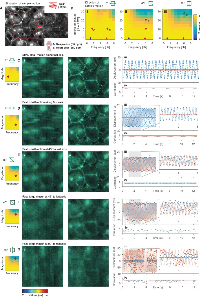
Figure 2. Evaluation of motion correction performance with simulated data.
(A) Illustration of generation of a frame in a simulated TTTR dataset. Main image shows high SNR intensity image used as the reference sample intensity. Red lines indicate the sample motion during the illustrated frame. Inset image shows the resultant simulated frame. (B) Average correlation coefficient over a range of magnitudes and frequencies of sinusoidal sample motion along an axis (i) 0°, (ii) 45° and (iii) 90°, respectively, from the fast axis. For comparison, indicative average values for the heart rate (red arrow, 350 bpm, 5.8 Hz) and respiration rate (blue arrow, 60 bpm, 1 Hz) of an adult mouse anaesthetized under ~1% isoflurane are shown. Black dots indicate results illustrated in the following panels. (C–G) Exemplar simulation results showing intensity merged lifetime images (i) without and (ii) with motion compensation. (iii) Estimated displacement traces in (blue) x and (red) y directions over time. In D-Giii, inset panels show expanded views of displacements between 1 and 3 s. (iv) Correlation between reference frame and (red) uncorrected and (blue) corrected images over time. Examples shown in C–E were corrected successfully, while the motion in examples F and G was too large to effectively compensate. (C) Motion parallel to fast axis with frequency 1.5 Hz and magnitude 10% of FOV. (D) Motion parallel to fast axis with frequency 6 Hz and magnitude 10% of FOV. (E) Motion at 45° to fast axis with frequency 6 Hz and magnitude 10% of FOV. (F) Motion at 45° to fast axis with frequency 6 Hz and magnitude 20% of FOV. (G) Motion at 90° to fast axis with frequency 6 Hz and magnitude 28% of FOV.


