Inverse Biomechanical Modeling of the Tongue via Machine Learning and Synthetic Training Data

Abstract

The tongue’s deformation during speech can be measured using tagged magnetic resonance imaging, but there is no current method to directly measure the pattern of muscles that activate to produce a given motion. In this paper, the activation pattern of the tongue’s muscles is estimated by solving an inverse problem using a random forest. Examples describing different activation patterns and the resulting deformations are generated using a finite-element model of the tongue. These examples form training data for a random forest comprising 30 decision trees to estimate contractions in 262 contractile elements. The method was evaluated on data from tagged magnetic resonance data from actual speech and on simulated data mimicking flaps that might have resulted from glossectomy surgery. The estimation accuracy was modest (5.6% error), but it surpassed a semi-manual approach (8.1% error). The results suggest that a machine learning approach to contraction pattern estimation in the tongue is feasible, even in the presence of flaps.

1. INTRODUCTION

Muscular contraction elicits tissue motion, which is necessary for a number of vital processes—for instance, cardiac contraction enables blood pressurization and tongue movement enables speech generation.^1,2 In the tongue, muscular activation patterns correspond to the spatial distribution of active tone (among several intrinsic and extrinsic muscles³), which generates the internal forces necessary to produce motion.² Activation patterns are sensitive to voluntary motion and reflexes, and can be affected by disease progression and procedures; thus, activation pattern characterization is of interest for improving our understanding of the processes on which the tongue is involved.^4–6

In the absence of methods for direct characterization, activation patterns can be estimated from electrical activity in the muscles, or inferred from tissue deformation extracted via tagged magnetic resonance imaging (MRI).^7,8 Imaging methods are considered less invasive and more reliable.⁸ The deformation-based estimation process comprises a forward biomechanical simulator and an iterative law that applies changes to the input of the simulations.⁹ The forward simulations output a deformation field given a candidate activation pattern, while the iterative law updates candidate patterns until there is agreement between the simulated and experimentally measured deformation. The process generally uses numerical optimization according to an objective metric.⁹ Because the update component makes deformation the input and contraction the output, this approach is known as inverse modeling.

Optimization-based inverse modeling must also require regularization to achieve a stable solution.⁹ For instance, the muscular mass can be subdivided into regions, which are assumed to contract uniformly and smoothly with respect to time.⁴ Regularization limits the number of possible activation patterns from which an estimated can be generated (the solution space); for instance, if muscular subdivisions are imposed, the output is limited to specific regions. Since accurate subdivisions are difficult to achieve in abnormal anatomy, there is a need for methods that can handle larger solution spaces, yielding more accurate solutions.⁹,¹⁵

In principle, machine learning approaches can enable the analysis of abnormal anatomy by including examples of abnormal activation patterns (and deformations) as training data.¹⁰ In lieu of direct observations of activation (not yet possible) and tongue deformation in patients, these data can be synthesized using a forward biomechanical model. That said, the set of contractions used for the training should be in some way feasible—and this requirement results in a constraint of the solution space similar to regularization in numerical optimization. However, unlike optimization (where regularization is necessary to achieve a stable solution), machine learning methods can be expanded almost arbitrarily. Although biomechanical model inversion via machine learning is promising, there are very few testing architectures that incorporate modeling, machine learning, and experimental data for training and regression.

In this paper, we illustrate a machine-learning pipeline for inverse simulation of tongue dynamics. The goal of the study is to present the basic concepts used to build the pipeline, demonstrating their compatibility with experimental data. Intuitively, given the number of muscles in the tongue at different contraction levels,³ the possible contraction configurations give rise to a massive solution space. For this reason, we also explore strategies for expanding the training database to eventually identify areas with contractile deficiencies (flaps).

2. METHODS

2.1 Inversion Pipeline

The proposed inverse modeling pipeline contains a machine-learning regression engine, a forward model, and a contractile pattern generator. Depending on its immediate use, these components can be configured for prediction or training, as shown in Fig. 1.

Figure 1.

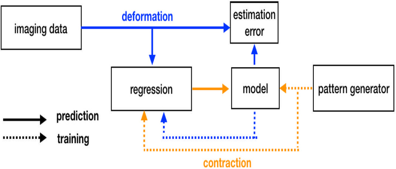
Inverse modeling pipeline. During regression, deformation information is extracted from imaging data to obtain contraction patterns. During training, contraction-deformation data pairs are generated by the contraction pattern generator in conjunction with the forward model.

In its prediction state, the pipeline outputs a contraction pattern based on a deformation field. Contractions are defined as forces along the local fiber orientation (i.e. projections of the stress tensor); these forces are normalized as a percentage of the maximum theoretical sarcomertic force.^11,12 Deformation fields consist of the local strain tensor (which is a tensorial measure of deformation) projected in the line of actions of local tissue fibers. Unlike contractile forces, strains and fiber orientations can be obtained experimentally from medical imaging via motion estimation and diffusion tensor MR, irrespectively.^7,8 Note also that strain patterns can be obtained from a simulation to verify accuracy. Predictions are generated using random forest (RF) regression,¹⁰ and was deployed via MATLAB scripts (v2005a, Mathworks, Natick, MA, USA) using the Statistics and Machine Learning Toolbox. The RF consisted of 30 decision trees with a depth of 5 observations, which operate independently on features corresponding to 262 contractile elements in Fig. 2. Since most elements contained two orthogonal fiber orientations the length of the strain-activation feature array was 524-by-2.

Figure 2.

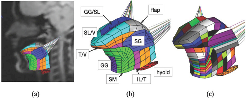
(a) In-vivo orientation of forward tongue model with 8 functional groups; (b) the forward tongue model with 8 uniformly-contracting groups modeled contraction of the superior longitudinal (SL), transversalis (T), verticalis (V), inferior longitudinal (IL), genioglossus (GG), styloglossus (SG), and support material (SM), while also designating some elements as non-contractile flaps; (c) tongue model with 262 independent functional elements (each colored uniquely).

During training, contraction data is used as an input to the forward simulator to obtain simulated deformation, and thus creating a contraction-simulation pair. The forward model was constructed using the FEBio Software suite.¹³ More information about tongue modeling including geometry, material directionality, material parameters, can be obtained in the literature.?^,9,15 Contraction data is generated using the contractile pattern generator, which can contain different application-specific synthesis approaches, which are referred henceforth as training schedules. Depending of the experiment detailed in the next Section, training schedules were designed based on a priori knowledge anatomical knowledge, arbitrary synthesis rules, or a combination of the two. Construction of training datasets is iterative, and termination is achieved by completion of a given number of training samples, or by approximating the amount of new information provided by each sample when compared to existing data.

2.3 Contraction Patterns from Tagged MRI

The goal of this experiment was estimating contraction patterns based on experimental data. Displacement information was obtained from a stack of tagged MRI images from a healthy volunteer using regularized harmonicbased analysis.^7,16 Tagged MRI images were acquired in a 3T scanner using a complementary spatial modulation of magnetization (CSPAMM) sequence, and comprised 10 coronal slices, 7 sagittal slices, 256 × 256 pixels at a resolution of 1.9×1.9 mm per pixel. The images were acquired as the volunteer pronounced the utterance ə-suk (“a-souk”). The time frames corresponding to each sound were identified by the timing of the acquisition.

The RF regression training schedule assumed a healthy muscle positioning and fiber orientations according to the literature.^3,17 Training was performed with a generic model based on a tongue atlas,¹⁸ which was later registered to the subject’s anatomy. The pattern generator was programmed to produce uniform contraction of 8 functional groups associated with 6 tongue muscles (Fig. 2b). The training data consisted of randomly sampling 50% of an equally spaced, 6-dimensional lattice, which represented combinatorial contraction of the muscles at 4 levels (4096 simulations). Data generation which took approximately 10 hours, and training took roughly 5 minutes.

The first step of the analysis was calibration to account for size differences between the generic and subject-specific model. Calibration focused on two time frames corresponding to /ə/ (the sound “uh” as in “hut”), which was the reference configuration, and /s/ (the “s” as in ‘sierra’)—the deformed configuration. Experimentally observed strains S_exp were fed to the RF regression assemble, and the resulting contractions were simulated using the forward model, which produced S_test. Error was calculated using

$$\epsilon =100\times \frac{\Vert \widehat{S}-S\Vert }{\Vert S\Vert },$$ (1)

where Ŝ is the estimate and S is the reference. Error, and the correlation between S_test and S_exp (with S_exp being the reference) were calculated to produce a scaling factor. This factor was obtained with and without averaging per muscle groups (i.e., using either of the models in Figs. 2b–c). The factor yielding the lowest error was kept for other time frames after calibration. For comparison, an additional simulation S_m of the calibration time frame was obtained using a semi-manual approximation of contraction as described in previous work.¹⁶

2.4 Activation Estimation with Contractile Deficiencies

The goal of this experiment was to test different training schedules for predicting contraction patterns with areas exhibiting contractile deficiency. These areas may be tissue grafts (flaps) introduced after tumor removal, or may arise from changes in innervation.¹⁹ It is assumed that either of these cases result in areas where no contraction occurs; thus, for simplicity, they are henceforth referred as flaps. It is also assumed that flaps are a subset of contraction patterns arising from those introduced in the previous section; Hence, the experiments were based on one seed contraction pattern without any flaps. The idea is that, in practice, the method in Section 2.3 can be used to achieve a coarse approximation of the overall contraction pattern (the seed), and the subset of data (versions of the seed containing flaps) can be used to refine the approximation in a second regression.

We aimed at characterizing prediction error as a function of the size of training datasets constructed following the training schedules described below. Initially, the training datasets contained the seed contraction pattern replicated a total of 50 times, which allowed setting up the minimum number of decision trees in the regressors (30) without any errors. The seed contraction pattern consisted of 32% contraction in the transversalis muscle, and 27% contraction in the verticalis muscle. The model shown in Fig. 2c was then used to generate training data according to the following training schedules (Fig. 3):

Figure 3.

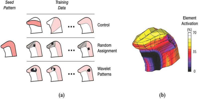
Training schedules for activation estimation with contractile deficiencies. The training approach schematic (a) shows the three training schedules. In the Control schedule, training data was added from patterns fundamentally different from the seed pattern. In Random Assignment, training data was generated from variations of the seed pattern, in which a flap was placed at random, either within a focused region (hashed area), or anywhere within the general seed pattern. Training using Wavelet Patterns were generated either focusing on a given region (white square), or the entire seed pattern (general variation). In the actual seed activation pattern (b), activation intensity varies with location.

1. Control

Data was added at random directly from the training dataset in Section 2.3. These data are largely dissimilar to the seed. The control dataset represents a type of worse-case scenario, since additional training data would not increase the accuracy of the regressor in cases with flaps.

2. Random Assignment

Training data was generated by modifying the seed contraction pattern by randomly selecting a group of neighboring elements within the tongue model and rendering it inactive. In other words, each discrete set of inactive elements models a discrete flap placed at random. This training schedule had two variations: random assignment of flaps within the middle third of the tongue, which is one of the most common location of tumors,²¹ and across all active muscles. These variations are respectively referred as focused and general.

3. Wavelet Patterns

The seed was projected from the FE model onto a grid, forming a pseudo-image of the seed contraction pattern. Then, the pseudo-image underwent a third-order wavelet decomposition, isolating geometrical features at different length scales. Wavelet coefficients associated with the size of the flap were modified using a random distribution. The resulting contraction pattern (a modification of the seed) was used to generate training data. This training schedule had the same (focused and general) variations described previously, which were implemented by applying wavelet transformations directly to the seed (general), or to a version of the seed with a flap (focused).

Training was terminated after a fixed number of new feature arrays were added to training data sets. Data generation ranged from 1–2 hours, and including time require for regressions on each iteration of new feature addition to the training data sets, the experiments ranged from 4–10 hours.

The training schedules were used to approximate contractions of five focused test cases. The focused test cases were kept separate from the training data, and represented versions of the seed contraction pattern with flaps. Percentage error was calculated using (1) applied across the entire tongue model. The Random Assignment training schedule was also tested using randomly assigned general test cases, since it is more useful for the regression to work in the general, rather than just the focused cases.

3. RESULTS AND DISCUSSION

3.1 Contraction Patterns from Tagged MRI

Preliminary activation estimates based on displacements from tagged images are illustrated in Fig. 4.

Figure 4.

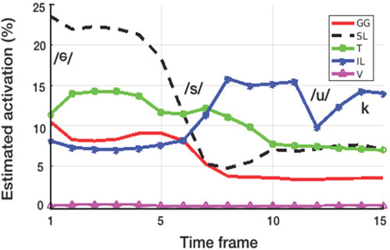
Regression output from imaging-based deformation measurements. The traces show activation percentages for the genioglossus (GG), superior longitudinalis (SL), transversalis (T), inferior longitudinalis (IL), verticalis (V) muscles. The first datapoint corresponds to the reference time frame.

The initial calibration error between S_exp and S_test was 6.3%—an improvement over the semi-manual approach, which yielded 8.1% error. Linear comparison between these solutions resulted in a slope of 1.3 (Pearson coefficient = 0.92), which suggests the activations were overestimated. After rescaling the activations and comparing to the experimental data, the calibration error was reduced to 5.6% (with a slope Pearson coefficient of 0.98 and 0.92, respectively). The approximation obtained without averaging muscular groups (Fig. 2c), resulted in 5.7% error—the lack of improvement was likely due to the training data itself, which originated form a model with eight independent muscles (Fig. 2b).

With the exception of the plot for the inferior longitudinalis, transition between sounds appeared smooth. Since no smoothness criteria was specified in the regression, this is likely a result of the image data. Earlier time frames suggest activity in the superior longitudinalins and transverse muscles, perhaps associated with extending the tongue into the “s” sound. The latter part of the utterance, appears to be dominated by activation of the inferior longitudinalis, which may play a role in the retraction needed for the “uk” sounds. The verticalis muscle appears to be inactive during the utterance; this result was unexpected as the tongue is expected to flatten during the “s” sound. Activation varyed from 0 to 24%. Altogether, it is still early to determine the precision and accuracy of the measurement, particularly because the prediction approach could compound error in motion estimation as well as in modeling. Therefore, it is difficult to describe the effectiveness of the regression pipeline in certain terms (other than predicting simulated states, which disregard modeling error). Nevertheless, this preliminary results show that it is possible to obtain an estimate of activation on which future work can build upon.

3.2 Flap Detection

3.2.1 Via Random Assignment Training

Fig. 5 shows how error changes as a function of the training data size. As expected, the control training schedule does not improve regression accuracy. In focused test cases, adding activation-contraction data from general flaps resulted in only marginal improvement in regression accuracy. Adding training data from focused flaps, however, resulted in more significant improvements in regression accuracy. This last approach caused approximately a 20% reduction in error. This result is expected, as the focused training data are more likely to have similarities with the focused test cases.

Figure 5.

Performance of the Random Assignment training schedule for predicting focused test cases.

When calculating error against general test cases, both the Control training schedule and the focused version of the Random Assignment training do not result in error improvement trends. With each random set of test cases, there is little likelihood for focused training data to coincide with the test cases. That said, after a somewhat long initial learning period (as general Random Assignment yields a large number of configurations), error estimation began to improve dramatically, decreasing by approximately 50% (Fig. 6). These results show that adding randomly-placed flaps to training data, being a more general approach, results in increased capability of approximating contractile deficiencies in a broader set of locations.

Figure 6.

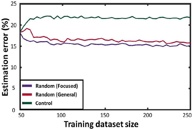
Performance of the Random Assignment training schedule for predicting general test cases.

3.2.2 Via Wavelet Pattern Training

Fig. 7a shows the evolution of error as a function of the relative size of the training database using both versions of the Wavelet Pattern training schedule. Unsurprisingly, control data did not result in any improvement on regression accuracy, and focused training was effective in detecting focused flaps with a trend showing improvement in approximation accuracy (20% error reduction). This suggests that perturbation of one of the test flaps can increase regression accuracy in other flap cases. The general training had no effect on the error trends. These results suggest that wavelet-based training can expand the overall regression capability, only if adequate seed patterns are carefully chosen to synthesize new data.

Figure 7.

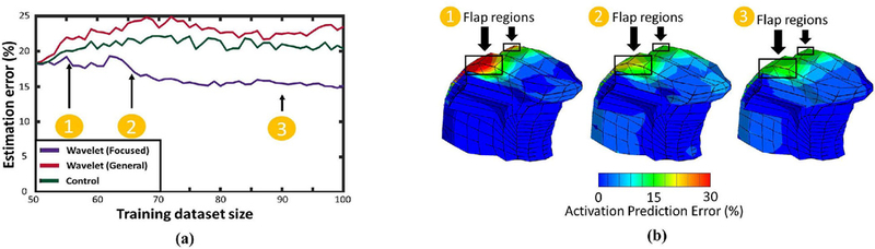
Regression accuracy under different training regimes. Augmenting the training data with perturbed flaps improves regression accuracy (a). This trend does not occur when adding perturbations of the original data, or random contraction-deformation pairs. The improvement is present in all 5 test cases, resulting in reduced error near the flap (b).

In general, we found that finding a randomly located flap in the most general case requires a colossal amount of training data. For instance, attaining a 50% error reduction from an initial guess (provided by the method in Section 2.3) would require augmenting each of the 2048 training samples from Section 2.3 with 72 additional data entries, resulting in a training data set of 149,504 entries! More research is necessary to determine precisely whether the error reductions justify these databases, how they relate to regularized optimization, and how can it be optimized. It is also possible that other machine learning methods, such as convolutional neural networks (CNNs),²⁰ are more effective. This is provided that CNNs are developed for FE kernels, which were not available at the time of this research. Nevertheless, this research shows that machine learning offers a relatively modular and expandable framework, which has potential for dealing with abnormal anatomical configurations.

4. CONCLUSION

This work described and demonstrated a pipeline for inverse biomechancial modeling using machine learning. Instead of assuming an explicit regularization scheme for stabilizing numerical optimization, the proposed approach can include a larger number of samples in the contraction-deformation space. However, as these samples ought to be feasible, the data must be subject to a form of implicit regularization. Our results indicate that the method is compatible with experimental data, and could be used in diseased states.

REFERENCES

- 1.Axel L, Montillo A, Kim D. Tagged magnetic resonance imaging of the heart: a survey. (2005) Medical Imaging Analysis 9(4):376-93. [DOI] [PubMed] [Google Scholar]
- 2.Gilbert RJ, Napadow VJ, Gaige TA, Wedeen VJ. Anatomical basis of lingual hydrostatic deformation.(2007) Journal of Experimental Biology 210(23):4069-82. [DOI] [PubMed] [Google Scholar]
- 3.Sanders I, Mu L. A three-dimensional atlas of human tongue muscles. (2013) Anatomical Record (Hoboken) 296(7):1102-14. [DOI] [PMC free article] [PubMed] [Google Scholar]
- 4.Harandi NM, Woo J, Stone ML, Abugharbieh R, Fels S. Variability in muscle activation of simple speech motions: A biomechanical modeling approach. (2017) Journal of the Acoustical Society of America 141:2579-2590. [DOI] [PMC free article] [PubMed] [Google Scholar]
- 5.Buchaillard S, Perrier P, Payan Y. A biomechanical model of cardinal vowel production: muscle activations and the impact of gravity on tongue positioning. (2009) Journal of the Acoustical Society of America 126(4):2033-51. [DOI] [PubMed] [Google Scholar]
- 6.Xing F, Ye C, Woo J, Stone M, Prince JL. Relating Speech Production to Tongue Muscle Compressions Using Tagged and High-resolution Magnetic Resonance Imaging. (2015) Proceedings of the International Society of Photo-Optical Instrumentation Engineers (SPIE) February;9413:94131L. [DOI] [PMC free article] [PubMed] [Google Scholar]
- 7.Osman NF, McVeigh ER, Prince JL. Imaging heart motion using harmonic phase MRI. (2000) IEEE Transactions on Medical Imaging 19:186202. [DOI] [PubMed] [Google Scholar]
- 8.Parthasarathy V, Prince JL, Stone ML, Murano EZ, Nessaiver M. Measuring tongue motion from tagged cine-MRI using harmonic phase (HARP) processing. (2007) Journal of the Acoustical Society of America 121(1):491-504. [DOI] [PubMed] [Google Scholar]
- 9.Stavness I, Lloyd JE, Fels S. Automatic prediction of tongue muscle activations using a finite element model. (2012) Journal of Biomechanics 45(16):2841-2848. [DOI] [PubMed] [Google Scholar]
- 10.Breiman L Random Forests. (2001) Machine Learning 45(1):5-32. [Google Scholar]
- 11.Guccione JM, McCulloch AD. Mechanics of active contraction in cardiac muscle: Part I-Constitutive relations for fiber stress that describe deactivation. (1993) Journal of Biomechanical Engineering 115(1):7281. [DOI] [PubMed] [Google Scholar]
- 12.Guccione JM, Waldman LK, McCulloch AD. Mechanics of active contraction in cardiac muscle: Part II-Cylindrical models of the systolic left ventricle. (1993) Journal of Biomechanical Engineering 115(1):8290. [DOI] [PubMed] [Google Scholar]
- 13.Maas SA, Ellis BJ, Ateshian GA, Weiss JA. FEBio: Finite elements for biomechanics. (2011) Journal of Biomechanical Engineering 134(1):011005. [DOI] [PMC free article] [PubMed] [Google Scholar]
- 14.Sanguineti V, Laboissiere R, Payan Y. A control model of human tongue movements in speech. (1997) Biological Cybernetics 77(1):11-22. [DOI] [PubMed] [Google Scholar]
- 15.Fujita S, Dang J, Suzuki N, Honda K. A computational tongue model and its clinical application. (2007) Oral Science International 4(2):97-109. [Google Scholar]
- 16.Gomez AD, Xing F, Chan D, Pham D, Bayly PV, Prince JL. Motion estimation with finite-element biomechanical models and tracking constraints from tagged MRI. (2017) Computational Biomechanics for Medicine: Algorithms Models and Applications 2017:81-90 [DOI] [PMC free article] [PubMed] [Google Scholar]
- 17.Takemoto H Morphological analyses of the human tongue musculature for three-dimensional modeling.(2001) Journal of Speech Language and Hearing Research 44(1):95-107. [DOI] [PubMed] [Google Scholar]
- 18.Woo J, Xing F, Lee J, Stone M, Prince JL. Construction of an unbiased spatio-temporal atlas of the tongue during speech. (2015) Information Processing in Medical Imaging 2015;24:723-32. [DOI] [PMC free article] [PubMed] [Google Scholar]
- 19.Edge SB, Compton CC. The american joint committee on cancer: the 7th edition of the AJCC cancer staging manual and the future of TNM. (2010) Annals of Surgical Oncology 17(6):1471-1474. [DOI] [PubMed] [Google Scholar]
- 20.Akkus Z, Galimzianova A, Hoogi A, Rubin DL, Erickson BJ. Deep learning for brain MRI segmentation: state of the art and future directions. (2017) Journal of Digital Imaging 30(4):449-459. [DOI] [PMC free article] [PubMed] [Google Scholar]
- 21.Goldenberg D, Ardekian L, Rachmiel A, Peled M, Joachims HZ, Laufer D. Carcinoma of the dorsum of thetongue. (2000) Head Neck 22(2):190-4. [DOI] [PubMed] [Google Scholar]