Standardized effect sizes for preventive mobile health interventions in micro-randomized trials

Abstract

Mobile Health (mHealth) interventions are behavioral interventions that are accessible to individuals in their daily lives via a mobile device. Most mHealth interventions consist of multiple intervention components. Some of the components are “pull” components, which require individuals to access the component on their mobile device at moments when they decide they need help. Other intervention components are “push” components, which are initiated by the intervention, not the individual, and are delivered via notifications or text messages. Micro-randomized trials (MRTs) have been developed to provide data to assess the effects of push intervention components on subsequent emotions and behavior. In this paper we review the micro-randomized trial design and provide an approach to computing a standardized effect size for these intervention components. This effect size can be used to compare different push intervention components that may be included in an mHealth intervention. In addition, a standardized effect size can be used to inform sample size calculations for future MRTs. Here the standardized effect size is a function of time because the push notifications can occur repeatedly over time. We illustrate this methodology using data from an MRT involving HeartSteps, an mHealth intervention for physical activity as part of the secondary prevention of heart disease.

Introduction

This paper addresses precision prevention through the development of a type of mobile health (mHealth) interventions called just-in-time adaptive interventions (JITAIs), which use an individual’s current mood, stress level, context, or behavior to provide tailored interventions that support positive behavior change. Mobile health interventions typically consist of several intervention components, such as tools for self-monitoring (e.g., graphs), reminders, educational materials, and so on. Some of these intervention components are “pull” components, in that they are accessed at will when the user decides that the component would be helpful. Pull components leave the user in control of the treatment, but their effectiveness depends on the user’s ability to determine when a particular component would be most useful and to remember to access intervention components at the times of need. Other intervention components are “push” components, which are sent by the intervention, not requested by the individual. Push components are usually provided as notifications or text messages, and common examples include reminders to perform self-care behaviors (e.g. to take medications), feedback on goal progress, and motivational messages. In traditional mHealth interventions, push components are typically provided based on a relatively simple set of decision rules. For instance, a medication reminder might be sent at the same time each day, or the intervention might send the user a motivational message if she missed her physical activity goal, measured in steps, three days in a row.

One problem with push components such as these is that they can be delivered in different contexts (e.g. in different locations or at different times of day), but they may not work equally well in all circumstances. For example, a reminder to take a medication might be ineffective if the individual is not at home and does not have the medication with her. Similarly, a message to help a person manage his nicotine craving that is intended to prevent smoking relapse might be more or less effective depending on whether the person is in a car, commuting home from work, or is at home on a weekend. In addition, push intervention components can interrupt and aggravate individuals during their daily lives, especially if the components arrive at inappropriate times or when they are not actionable (Smith et al., 2017). In response, individuals may disengage from the intervention over time, or delete the mHealth application altogether. Ideally, then, push components should be delivered with precision, at moments when they are most needed by the individual and when the individual is receptive to treatment (Nahum-Shani et al., 2016).

JITAIs are a class of mHealth interventions that attempt to tailor push intervention components to the individual’s current context, behavior, and physiological and psychological states in order to maximize their effectiveness and minimize user burden. To design these precise interventions, prevention scientists need to understand how the effectiveness of specific push components varies among individuals, across different contexts and treatment histories, and over time. The micro-randomized trial (MRT) is a new trial design that provides data to answer these questions and to inform decisions about whether and in which contexts push intervention components should be provided (Klasnja et al., 2015). This trial design provides data for investigating whether a push intervention component has an effect, how that effect changes across a series of treatment occasions, and how that effect is influenced by the “state” (the individual’s stress level, context, etc.) in which the intervention component is delivered. In this way, evidence from MRTs can help prevention scientists decide precisely when and where a particular intervention component should be delivered (or not delivered) to maximize its effectiveness and minimize user burden.

One statistical tool for evaluating intervention components using data from an MRT is the standardized effect size. A standardized effect size estimate can help scientists compare and select intervention components that might be included in a preventive mHealth intervention. In addition, standardized effect sizes can facilitate sample size calculations, meta-analyses, and rules of thumb for “small” and “large” effect sizes in mobile health. Indeed, standardized effect size estimates have been recommended as part of statistical analyses for decades (e.g. Wilkinson, 1999). Here we develop a method for using MRT data to form a standardized effect size estimate for mHealth intervention components that can be delivered repeatedly and may have varying effects over time.

This paper reviews the MRT design, motivates and describes a standardized effect size calculation for MRTs, and illustrates the MRT design and standardized effect size using a study of HeartSteps, a mobile intervention designed to improve physical activity as part of the secondary prevention of heart disease. For clarity we begin with a description of HeartSteps.

Example: HeartSteps

We are developing a mobile health intervention, HeartSteps, that encourages individuals to be physically active. The final version of HeartSteps will be a secondary prevention intervention to decrease the likelihood of subsequent adverse cardiac events among individuals with cardiovascular disease. In this paper we focus on the first of three micro-randomized trials designed to inform the development of HeartSteps.

The first trial for HeartSteps was a 42-day study involving 44 sedentary adults. The participants were provided Android smartphones and wore a Jawbone Up Move wristband that recorded their step count every minute. Sensors on the smartphones collected contextual information including each participant’s location (classified as home, work, or “other”), current weather, and current activity classification (sedentary, walking, running, or potentially operating a vehicle). In addition, each evening, participants were asked to reflect on their day with questions about how stressful, typical, and hectic the day was.

One of the intervention components tested in this initial trial of HeartSteps was daily planning of physical activity. Each evening, as part of the evening reflection questions, participants might be prompted to create a plan for how they would be active during the following day. This intervention component embodied the construct of implementation intentions (Gollwitzer, 1999), which are specific plans for when, where, and how an activity will be performed. Implementation intentions have previously been used to support physical activity habits during cardiac rehabilitation (Luszczynska, 2006) and have been shown to be effective at initiating a range of health-promoting behaviors (Gollwitzer, 1999). We are interested in the effect that creating an activity plan has on the following day’s step count. This planning intervention component will be discussed at greater length below, when we describe the micro-randomized trial design and illustrate our standardized effect size calculation using data from the HeartSteps trial.

Micro-randomized trials

The micro-randomized trial (MRT) is a randomized trial design for use in estimating the effects of push intervention components that might be delivered repeatedly over time. Examples of push intervention components include motivational messages, behavioral suggestions to take one’s mind off a craving and prevent relapse, or messages that help reframe a lapse to a health-risk behavior. In an MRT, participants are randomly assigned to different options for a given intervention component at each of many decision points. The decision points are times at which it might be appropriate to deliver the intervention component. At each decision point in an MRT, each participant is randomized to receive a specific version of an intervention component, such as different framings for motivational messages, or to receive no treatment.

In HeartSteps the decision points for the activity planning component occurred once per day: each evening as part of the daily reflection questions. At each decision point, that is, each evening, participants were randomly assigned to receive or not receive (each with probability 0.5) the prompt to create an activity plan for the following day. Those receiving this intervention component were asked to plan their physical activity for the following day in either an unstructured or a structured format (each with probability 0.5). Unstructured planning required free text entry of a plan for the next day’s activity while structured planning required the participant to select from a tailored menu of options (see Figure 1).

Figure 1.

Screenshot of the unstructured daily planning component (left panel) and the structured daily planning component (right panel) in the study of HeartSteps.

By randomizing participants many times over the course of a study, MRTs enhance scientists’ ability to estimate the causal effects of time-varying mobile health intervention components as well as moderated effects of these time-varying components. Data from an MRT can reveal whether an intervention component is effective as well as the circumstances or context under which it is effective. The micro-randomized trial is thus a powerful experimental tool for developing precision-based, preventive JITAIs, as it provides an empirical basis for decisions about when intervention components should and should not be delivered. For example, using data from the HeartSteps MRT, we can estimate the effect of each type of planning activity (unstructured or structured) on the following day’s step count and determine whether this effect depends on whether the plan is created for a weekday or a weekend, the number of steps taken on the current day, and individual characteristics such as gender.

The causal effects estimated in an MRT, and hence the evidence an MRT provides about the efficacy of mobile health intervention components, rely on the notion of a proximal outcome. A proximal outcome reflects the short-term desired effect of a single administration of an intervention component. Often, proximal outcomes are postulated mediators on the path from the component to a distal outcome of interest. For example, an mHealth intervention for adolescents at high risk of substance abuse might involve reminders to practice stress-reducing mindfulness exercises, with the long-term goal of preventing substance use. In this case a proximal outcome might be the fraction of time the participant is stressed in the two hours following the decision point, while the distal outcome might be the time until substance use. For the daily planning component in HeartSteps, the proximal outcome is the following day’s step count and the distal outcome is the average daily step count. Thus, in HeartSteps, the proximal outcome directly contributes to the distal outcome. Data from an MRT are used to estimate the causal effects of specific intervention components on proximal outcomes. For further discussion of MRTs see Klasnja et al. (2015), Liao, Klasnja, Tewari, and Murphy (2016), and Dempsey, Liao, Klasnja, Nahum-Shani, and Murphy (2015).

In the following two sections, we will describe a standardized effect size estimate for the effect of an mHealth intervention component on a proximal outcome in an MRT. Since participants in an MRT are repeatedly randomized, that is, delivery of the mHealth intervention component is time-varying, this standardized effect size is a function of time describing how the effect of an intervention component changes across a sequence of decision points when that component might be delivered.

Treatment effects and standardized treatment effects

In this section we provide a conceptual description of the treatment effects investigated in a micro-randomized trial and discuss changes in these effects over the course of a study. We then introduce our standardized effect size calculation. For clarity, we consider only two treatment options at each decision point (receiving an intervention component versus not receiving the component) and a continuous proximal outcome. At each decision point, the effect of treatment (an intervention component) is the mean difference in a proximal outcome between treated and untreated participants at that decision point. Technically, let t = 1, …, T index decision points with A_t = 1 if the participant was treated and A_t = 0 if not. Denote the proximal outcome following decision point t as Y_t+1. In HeartSteps, for example, the decision points for the planning component occurred each evening and Y_t+1 is the following day’s step count. The effect of treatment at decision point t is the expected difference in Y_t+1 between treated and untreated participants, namely,

$$\beta (t)=\mathrm{E}[Y_{t+1}|A_t=1]-\mathrm{E}[Y_{t+1}|A_t=0].$$ (1)

See Liao et al. (2016) for a full derivation of β(t) using causal inference notation. Notice that β(t) is the proximal effect of delivering a treatment at decision point t, as opposed to a time-varying, longitudinal, effect of a single treatment administered at baseline. The decision point index t represents time since the first randomization.

There are several reasons why the treatment effect, β(t), might change across the repeated randomizations in an MRT. Since intervention components in an MRT are provided on many occasions over days or weeks, participants might start to habituate (ignore) those components. Or their enthusiasm for improving physical activity might be high at the start of the trial and diminish over time. In these cases it is plausible that the treatment effect for intervention components provided at earlier decision points would be higher than the treatment effect at later decision points. Seasonal changes during the study period could also moderate the effects of the intervention components, especially in a study like HeartSteps, where the health behavior of interest (physical activity) likely depends on the weather.

Effect sizes for micro-randomized trials

A standardized effect size for the micro-randomized trial is the magnitude of the effect of an intervention component on the proximal outcome relative to the variability in the proximal outcome. Since the effect of receiving an intervention component may differ at each decision point in an MRT, a single standardized effect size statistic is an inadequate description of treatment efficacy. Here we provide a standardized effect size expressed as a function of time so as to reflect changes in the magnitude of the proximal treatment effect across the sequence of decision points in an MRT.

A natural effect size measure at a single decision point t is the standardized mean difference

$$d(t)=\frac{\beta (t)}{\sigma (t)}$$ (2)

where σ(t) is the population standard deviation of Y_t+1. This is Cohen’s d (Cohen, 1988) and measures the magnitude of the treatment effect in standard deviation units. Typically, the standard deviation estimate in Cohen’s d is a pooled estimate calculated assuming the two treatment groups have the same standard deviation. In this discussion we will use the pooled standard deviation as the denominator of d(t) (see Olejnik and Algina (2000) for other methods of standardizing a mean difference effect size).

Estimating the standardized effect size as a function of time

First we review how to estimate the standardized effect, d(t), at a single decision point. The standardized effect size for an intervention component in an MRT, expressed as a function of time, will be computed using estimates of d(t) from all decision points. A straightforward estimate of d(t) at decision point t is

$$d_{\mathrm{s}}(t)=\frac{b(t)}{s_{\text{pool}}(t)}$$ (3)

with

$$b(t)={\overline{Y}}_{t+1,1}-{\overline{Y}}_{t+1,0}$$

$$s_{\text{pool}}^2(t)=\frac{(n_{t,0}-1)s_0^2(t)+(n_{t,1}-1)s_1^2(t)}{n_{t,0}+n_{t,1}-2}$$

$${\overline{Y}}_{t+1,a}=\text{sample}\text{mean}\text{of}{Y}_{t+1}\text{for}\text{participants}\text{with}{A}_t=a$$

$$s_a^2(t)=\text{sample}\text{variance}\text{of}{Y}_{t+1}\text{for}\text{participants}\text{with}{A}_t=a$$

$$n_{t,a}=\text{number}\text{of}\text{participants}\text{with}{A}_t=a$$

Other choices are possible for b(t), an estimate of β(t). It is typical to adjust for pre-decision point covariates when estimating β(t) instead of using the unadjusted sample mean ${\overline{Y}}_{t+1,1}-{\overline{Y}}_{t+1,0}$. In a micro-randomized trial, one natural pre-decision point covariate is the prior decision point’s proximal outcome. Denote the prior decision point’s proximal outcome measurement as Z_t. Consecutive proximal outcomes in an MRT are within-person measurements within relatively short time intervals, so one expects a high degree of correlation between Z_t and Y_t+1. We therefore adjust for Z_t by using as our estimate of β(t) the coefficient for A_t from a regression model with response variable Y_t+1 and covariates A_t and Z_t. Note that this regression model uses the cross-sectional data from decision point t, where A_t is the treatment variable and Z_t is a covariate measured before the decision point.

Once standardized effect sizes are computed at every decision point, we combine these estimates to obtain a standardized effect size that can be displayed as a smooth function of time. Smoothing techniques such as LOESS, smoothing splines, and kernel smoothers (e.g. Friedman, Hastie, & Tibshirani, 2009) are well suited to this task. With dozens or hundreds of decision points in an MRT, these smoothing techniques will produce similar function estimates for the standardized effect size. Here we use LOESS with degree-1 polynomials (Cleveland & Devlin, 1988). For additional technical discussion of these smoothing techniques, see the supplemental materials (available online). To obtain the standardized effect size as a smooth function of time, we apply LOESS separately to b(t), the estimated treatment effect, and to s_pool(t), the pooled standard deviation, across all decision points. This produces estimates of these quantities as functions of time since the first decision point, and the final standardized effect size function is the ratio of these two function estimates. We apply LOESS separately to b(t) and s_pool(t) because simulation results (available online) suggest that this procedure has less bias and greater precision than applying LOESS to the ratios d_s(t).

To describe the uncertainty in this standardized effect size function, we compute bootstrap confidence intervals (Efron & Tibshirani, 1994, Chapter 13) at each point for which the effect size function is displayed. This is done by repeatedly sampling the participants to create many bootstrap samples. For each bootstrap sample, the same standardized effect size function is computed. The 90% confidence limits at a decision point are the sample 95th and 5th percentiles from this set of bootstrap effect size functions evaluated at that decision point.

Example: standardized effect sizes for activity planning in HeartSteps

In this section we illustrate the calculation of standardized effects sizes using HeartSteps. We also illustrate how these standardized effects sizes can be used in a subsequent study to further develop HeartSteps. Recall that participants in the HeartSteps trial received the planning component each evening with probability 0.5. There were two formats for the planning component. In unstructured planning, participants were given an example activity plan and then asked to enter their plan for the following day in an open text box. In addition, at the start of the study, participants were instructed to be specific when writing their activity plans, including the time and location when they would complete the physical activity. In the structured planning format, participants were asked to choose from a list of plans they had entered in the text box on prior days. See Figure 1 for examples of these two formats. We were interested in investigating these two planning formats because they both target the same construct—implementation intentions—but with different potential benefits and drawbacks. Unstructured planning is flexible, as it enables participants to devise plans that are tailored to their upcoming day and to be mindful while they are planning, but it is also laborious. Structured planning, on the other hand, is much less work for participants, since they can simply pick a planning option from a list. Insofar as participants’ daily lives are often routine, this planning format should still allow them to pick plans that are relevant and actionable. However, choosing a predefined plan requires less attention compared to creating a new plan. We were thus interested in studying how these differences between the two planning formats influence their effectiveness and influence participants’ experience of the intervention. For participants assigned to receive the planning component, a single planning format (unstructured or structured) was assigned with probability 0.5. In evaluating the unstructured and structured planning components, we were primarily interested in their effect on the following day’s step count. We were also interested in the effect of creating an activity plan when the following day is a weekday, since individuals’ activity patterns are often different between weekdays and weekends.

Computing the standardized effect size function

Recall that the decision points, t, for the activity planning components occurred during the evening of each study day. The daily step counts were square-root transformed to obtain a more symmetric distribution, so the proximal outcome, Y_t+1, for the planning component is the square-root daily step count on the following day. The prior decision point’s proximal outcome, Z_t, is the square-root daily step count for the same study day (the day before the plan is meant to be carried out). As an example, consider a participant who is randomly assigned to create an activity plan on Tuesday evening, so that A_t = 1 and t is the index value for Tuesday evening’s decision point. For this participant, Y_t+1 is her square-root step count on Wednesday and Z_t is her square-root step count on Tuesday.

In the following standardized effect size calculations, data from 7 of the 44 participants in the HeartSteps trial were excluded: 3 participants used phones set to a non-English locale, resulting in corrupted data; 2 participants dropped out within 4 days due to unfamiliarity with the Android phones provided in the trial; and the final 2 participants dropped out within 2 weeks. The remaining 37 participants were enrolled in the study for a combined 1,529 days (at most 42 days per participant). In the following calculations, we only include the decision points t for which Z_t, the prior decision point’s proximal outcome, and Y_t+1, the proximal outcome, are not missing. This eliminates 415 decision points that occurred while the participants were traveling or experiencing technical problems with their phones or wristbands as well as 37 decision points from each participant’s first study day, when there is no prior decision point and hence no value for Z_t. Finally, we exclude the 37 decision points from the second study day because only partial step counts were recorded on the first study day. This leaves a total of 1,040 decision points across the 37 participants included in this illustrative analysis.

First we will compute standardized effect sizes for two contrasts: unstructured planning versus no planning treatment; and structured planning versus no planning treatment. Second, because the unstructured planning component shows promise in improving physical activity (see below), we computed the standardized effect size for unstructured planning for weekdays versus no planning treatment for weekdays. We omit standardized effect sizes for activity plans created for weekends because in the pilot study there were few weekends per participant and thus we have very little data concerning the effect of the activity plans on weekend step counts.

To demonstrate the intermediate calculations required to obtain the standardized effect size function, the left panel of Figure 2 displays estimates of the effect of the unstructured planning component on the square-root daily step count for each decision point t. Recall that the estimate b(t) at each decision point is the coefficient for A_t from an ordinary least squares regression model with response variable Y_t+1 and covariates Z_t and A_t. In this case, A_t = 1 if the participant received the unstructured planning component and A_t = 0 if the participant received no planning treatment. The right panel of Figure 2 displays the pooled standard deviation of Y_t+1 for each decision point. All of the estimates in Figure 2 are separately computed using the cross-sectional data from each decision point. The curves in Figure 2 are LOESS regression functions for the estimates b(t) and s_pool(t), and the standardized effect size function for the unstructured planning component is the ratio of these two curves.

Figure 2.

Estimates of β(t) (left panel) and pooled standard deviations (right panel) for the unstructured planning component for each decision point in the study of HeartSteps. The curves are degree-1 LOESS regression functions.

Figure 3 displays standardized effect size functions for the unstructured and structured planning components. These effect sizes suggest little or no effect of creating a structured plan on the next day’s physical activity and a small, positive effect of creating an unstructured plan, which becomes somewhat larger near the end of the study period. The estimated treatment effect for the unstructured planning component on study day 40 seems unusually high, so we recomputed this standardized effect size without the estimated treatment effect on study day 40; the qualitative results of the computation did not change. Sensitivity analyses such as this one, along with confidence intervals, can ensure an appropriately cautious interpretation of these standardized effect size functions.

Figure 3.

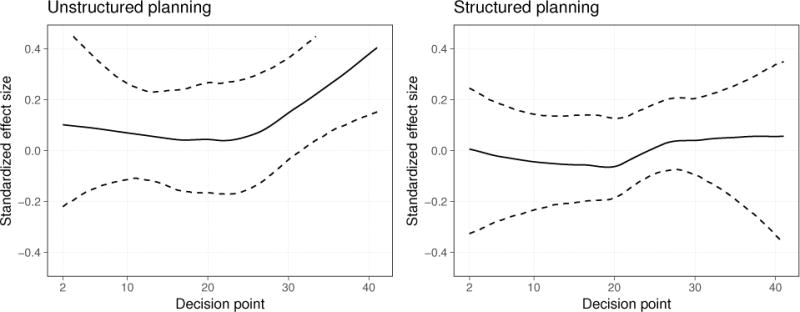
Time-varying standardized effect size for the unstructured planning component (left panel) and the structured planning component (right panel) in the study of HeartSteps. The dashed lines are 90% bootstrap confidence intervals computed with 5,000 bootstrap samples from the 37 participants in this analysis.

We were also interested in whether the activity plans had an effect specifically when the plans were created for a weekday. Figure 4 illustrates a standardized effect size function motivated by this interest, namely, that of the unstructured planning component using only decision points for which the next day is a weekday. This effect size is larger than those of the unstructured and structured planning components computed using all decision points (Figure 3), remaining roughly constant near 0.2 for the duration of the study.

Figure 4.

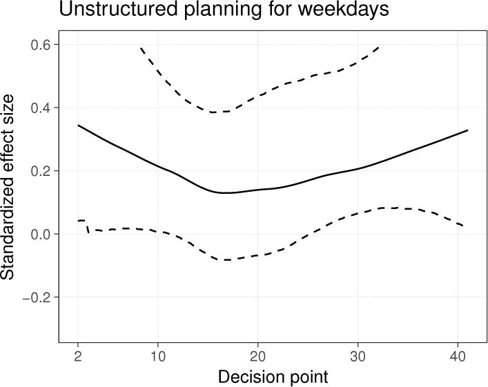
Time-varying standardized effect size for the unstructured planning component in the study of HeartSteps, using only the decision points for which the next day is a weekday. The dashed lines are 90% bootstrap confidence intervals computed with 5,000 bootstrap samples.

These standardized effect size functions are intended to accompany main effects analyses for each intervention component. Statistical hypothesis tests for the unstructured planning component in this pilot study suggested that it may have a marginal proximal effect on participants’ step counts and prompted further investigation of its marginal effect on weekdays. These standardized effect sizes complement main effects analyses for the unstructured planning component by estimating the magnitude of its proximal treatment effect over time. As illustrated in the following two sections, this provides empirical support for intervention design and the planning of future MRTs. The confidence intervals for all three of the standardized effect size functions are quite wide, with interval widths close to 0.4. This is not surprising, since just 37 participants were included in this study, and suggests that we have limited information on small fluctuations in the standardized effect over time and that we should use a conservative estimate of the standardized effect when conducting power analyses.

Using standardized effect size functions to inform future development of HeartSteps

The above calculations are useful in furthering the development of an mHealth intervention such as HeartSteps as well as in the design of future MRTs. First, the effect size calculation does not provide evidence that the structured planning component is useful. However, the unstructured planning component does appear useful in improving physical activity, particularly on weekdays. This motivates including only unstructured planning in future versions of HeartSteps. Furthermore, suppose that participants report in exit interviews that creating the unstructured activity plans is onerous even though the above results indicate that these unstructured plans hold promise for improving physical activity on weekdays. Suppose further that a follow-up trial will last three months and we wish to reduce participant burden while still providing the unstructured planning component. In the follow-up study, we could prompt participants, on evenings that precede a weekday, to create an unstructured plan with probability 0.4, leading to an average of two unstructured plans per week for each participant (since there are five weekdays per week). With these design considerations in mind, we can now use the methodology developed in Liao et al. (2016) and Seewald, Sun, and Liao (2016) to compute the sample size required to detect a given standardized treatment effect for the unstructured planning component in such a follow-up study.

For this sample size calculation, we need to specify the following: the study duration in days; the number of decision points per day; the randomization probability for the intervention component; and an average (across time) standardized treatment effect with a time-varying pattern (e.g. constant or linearly decreasing) for this treatment effect. The standardized effect size developed in this paper provides an empirical method for specifying the standardized treatment effect, and its time-varying pattern, to size future MRTs. Note that many time-varying patterns are possible for a given average standardized treatment effect; refer to Liao et al. (2016) for further illustration. (We also require a quantity called the expected availability of participants for treatment, expressed as a probability. Since the evening planning component is scheduled at a participant-specified time, the expected availability is 1. See Klasnja et al. (2015) and Liao et al. (2016) for a discussion of participant availability.) Continuing our example, we refer to the graph of the effect size for unstructured planning on weekdays (Figure 4) to specify an average standardized treatment effect. In this case, the average standardized treatment effect is roughly 0.2 with a constant pattern over time (in describing this effect as constant over time, we have incorporated our uncertainty about this effect size as measured by the confidence intervals in Figure 4). In a three-month study, there will be 60 decision points that occur on evenings that precede a weekday. With a randomization probability of 0.4, the sample size required to detect a constant treatment effect of 0.2 with 80 percent power at significance level 0.05 is 17 participants. If instead we specify a constant standardized effect size of 0.15 and 90 percent power, the required sample size is 35 participants. Alternatively, to obtain an average of one activity plan (for weekdays) per week, we would randomize the planning component with probability 0.2. Then, with a constant standardized treatment effect of 0.15 and 90 percent power, the required sample size is 51 participants. These calculations were performed using the software described in Seewald et al. (2016), which can be accessed at https://pengliao.shinyapps.io/mrt-calculator/.

Discussion

The micro-randomized trial allows behavioral scientists to investigate the causal effects of time-varying push intervention components in an mHealth intervention and the contextual moderators of those effects, thus enabling the construction of precision JITAIs for positive behavior change and prevention of adverse health outcomes. The standardized effect size developed in this paper displays, as a function of time, the magnitude of proximal treatment effects for intervention components that can be delivered at each of many decision points in an MRT. In addition to enabling sample size calculations based on empirical estimates of standardized treatment effects over time, as we illustrated above with HeartSteps, this standardized effect size will help scientists decide which intervention components should be included in an mHealth intervention and when those components should be provided to specific people.

The MRT of HeartSteps illustrates this point. In this trial, the standardized effect size for the structured planning component was very small throughout the study period (Figure 3), suggesting that this component is ineffective for helping individuals increase their physical activity. For this reason, the next version of HeartSteps will not include a structured planning component. The standardized effect sizes for the unstructured planning component (Figures 3 and 4), on the other hand, along with primary analyses for this component (omitted here for brevity), suggested that unstructured planning might be an effective treatment, especially when it asks individuals to plan their physical activity for a weekday. These findings motivated retention of unstructured activity planning in the next version of HeartSteps, as well as the decision to only provide this component on evenings that precede a weekday.

What is important to note, however, is that effect size estimates from MRTs do not automatically translate into selection of intervention components or the decision rules for their provision. Inclusion of any intervention component in a JITAI presents a set of trade-offs, and effect sizes form just one of many factors that have to be considered when designing a JITAI. Again consider HeartSteps as an example. The next HeartSteps trial will last three months, and the trial after that will last one year. In such studies where a JITAI has to be used over an extended period of time, inclusion of intervention components, even if they have a statistically “significant” proximal treatment effect, must be weighed against their potential for producing clinically meaningful improvements in health behaviors and for inflicting excessive burden on users of the intervention. For instance, the standardized effect size for another intervention component in HeartSteps, which provided contextually tailored suggestions for physical activity up to five times each day, indicated that the effect of this component was strong initially but deteriorated over the course of the study. Even though a hypothesis test for the marginal effect of this component had a p-value below 0.05, including the component in a longer study without modification would almost certainly fail. This is because the beneficial effects of this component would likely disappear early in the study and because repeated provision of suggestion messages would increasingly annoy participants, risking their disengagement with the intervention as a whole. For these reasons, for the next HeartSteps trial, we will reduce the frequency of activity suggestions and schedule week-long periods with very few suggestion messages so that the beneficial effect of the intervention component might be sustained over a longer period of time. The standardized effect size calculation presented here can provide empirical evidence for such considerations about intervention design.

Returning to our example of daily planning in HeartSteps, we expected prior to conducting this trial that the standardized effect sizes for this component would decrease over time due to participant burden and habituation to the planning activities. Somewhat surprisingly, this did not occur based on the effect sizes presented here. However, the bootstrap confidence intervals for the planning effect sizes lead us to believe that the apparent increase in the effect of this component near the end of the study is due to sampling variability. Standardized effect sizes presented as a function of time can assist in assessing possible changes in the effect of intervention components over time.

Another potential use of standardized effect sizes from MRTs is to begin to establish rules of thumb for small or large effects in mobile health and, thus, to provide guidance for which intervention components are worth investigating further. To make this possible, however, more studies are needed to assess the connection between standardized effect sizes for proximal outcomes and their impact on distal clinical outcomes. Our expectation prior to computing standardized effect sizes for the study of HeartSteps was that the suggested magnitudes for small and large effect sizes provided by Cohen (1992) would be far too large for treatment effects for proximal outcomes in mobile health. This is because, at each decision point, the standardized effect size function for MRTs describes the effect on a proximal outcome of a single administration of an intervention component, such as a single session of activity planning. However, the results presented here suggest that standardized effect sizes in MRTs may be similar in magnitude to standardized effect sizes for traditional trial designs. Whether this also means that Cohen’s heuristic standards for small, medium, and large effects will hold for MRTs is unclear, however. Additional data are needed before rules of thumb can be developed to evaluate results from micro-randomized trials and to predict clinical usefulness of individual intervention components. It might be that a standardized effect size of 0.4 or 0.5 for a single proximal outcome can be observed alongside minimal changes in distal clinical outcomes. On the other hand, since the standardized effect size function for an MRT describes the proximal effect of an intervention component that is delivered many times, a small effect size that is consistent over time, like the one observed for the unstructured planning component in HeartSteps, might produce a clinically meaningful impact on a distal outcome. More data are needed to understand the relationship between proximal effect sizes observed over time and their impact on clinical outcomes.

The JITAI framework holds a great deal of promise for designing effective prevention interventions that provide highly tailored support when the individual most needs it and is most likely to benefit from it. For instance, the mobile intervention BASICS-MOBILE (Witkiewitz et al., 2014) sought to reduce heavy drinking and smoking among college students. The intervention prompted participants to assess, among other measures, their smoking urge and affect three times per day and sent an urge-surfing (Bowen & Marlatt, 2009) component when participants reported an urge to smoke. A JITAI following this approach might use geofencing to detect that a college student is approaching a store where he has regularly purchased cigarettes in the past, or detect, using wearable sensors, that he is stressed and hence may have an urge to smoke. The JITAI could then send him a reminder of his goals for reducing tobacco use and a tailored message to help him avoid the temptation to smoke. Similarly, the cStress model for detecting stress episodes (Hovsepian et al., 2015), during which there may be increased risk of relapse, is being used in a smoking cessation JITAI to trigger stress-reducing intervention components (Kumar et al., 2017).

Construction of such precise, preventive JITAIs will require investigators to efficiently identify effective intervention components and determine the contexts in which they are most effective for specific individuals. As illustrated by our discussion of the HeartSteps trial, micro-randomized trials can help assess the causal moderated effects of intervention components and, through the use of standardized effect sizes, can describe the magnitude of those effects across a series of treatment occasions. This enables investigators to identify promising intervention components and to formulate decision rules for their optimal provision. The work we presented here further extends the usefulness of the micro-randomized trial design by enabling comparisons of the effectiveness of different intervention components and investigation of the relationships between the proximal effects of push interventions and distal health outcomes.

References

- Bowen S, Marlatt A. Surfing the urge: brief mindfulness-based intervention for college student smokers. Psychology of Addictive Behaviors. 2009;23(4):666. doi: 10.1037/a0017127. [DOI] [PubMed] [Google Scholar]
- Cleveland WS, Devlin SJ. Locally weighted regression: An approach to regression analysis by local fitting. Journal of the American Statistical Association. 1988;83(403):596–610. [Google Scholar]
- Cohen J. Statistical power analysis for the social sciences. Hillsdale, NJ: Erlbaum; 1988. [Google Scholar]
- Cohen J. A power primer. Psychological bulletin. 1992;112(1):155. doi: 10.1037//0033-2909.112.1.155. [DOI] [PubMed] [Google Scholar]
- Dempsey W, Liao P, Klasnja P, Nahum-Shani I, Murphy SA. Randomised trials for the fitbit generation. Significance. 2015;12(6):20–23. doi: 10.1111/j.1740-9713.2015.00863.x. [DOI] [PMC free article] [PubMed] [Google Scholar]
- Efron B, Tibshirani R. An introduction to the bootstrap. Taylor & Francis; 1994. [Google Scholar]
- Friedman J, Hastie T, Tibshirani R. The elements of statistical learning. Springer-Verlag; New York: 2009. [Google Scholar]
- Gollwitzer PM. Implementation intentions: strong effects of simple plans. American psychologist. 1999;54(7):493. [Google Scholar]
- Hovsepian K, al’Absi M, Ertin E, Kamarck T, Nakajima M, Kumar S. cstress: towards a gold standard for continuous stress assessment in the mobile environment. Proceedings of the 2015 acm international joint conference on pervasive and ubiquitous computing. 2015:493–504. doi: 10.1145/2750858.2807526. [DOI] [PMC free article] [PubMed] [Google Scholar]
- Klasnja P, Hekler EB, Shiffman S, Boruvka A, Almirall D, Tewari A, Murphy SA. Microrandomized trials: An experimental design for developing just-in-time adaptive interventions. Health Psychology. 2015;34(S):1220. doi: 10.1037/hea0000305. [DOI] [PMC free article] [PubMed] [Google Scholar]
- Kumar S, Abowd G, Abraham WT, al’Absi M, Chau DH, Ertin E, Wetter D. Center of excellence for mobile sensor data-to-knowledge (md2k) IEEE Pervasive Computing. 2017;16(2):18–22. doi: 10.1109/MPRV.2017.29. [DOI] [PMC free article] [PubMed] [Google Scholar]
- Liao P, Klasnja P, Tewari A, Murphy SA. Sample size calculations for micro-randomized trials in mhealth. Statistics in Medicine. 2016;35(12):1944–1971. doi: 10.1002/sim.6847. [DOI] [PMC free article] [PubMed] [Google Scholar]
- Luszczynska A. An implementation intentions intervention, the use of a planning strategy, and physical activity after myocardial infarction. Social science & medicine. 2006;62(4):900–908. doi: 10.1016/j.socscimed.2005.06.043. [DOI] [PubMed] [Google Scholar]
- Nahum-Shani I, Smith SN, Spring BJ, Collins LM, Witkiewitz K, Tewari A, Murphy SA. Just-in-time adaptive interventions (JITAIs) in mobile health: Key components and design principles for ongoing health behavior support. Annals of Behavioral Medicine. 2016:1–17. doi: 10.1007/s12160-016-9830-8. [DOI] [PMC free article] [PubMed] [Google Scholar]
- Olejnik S, Algina J. Measures of effect size for comparative studies: Applications, interpretations, and limitations. Contemporary educational psychology. 2000;25(3):241–286. doi: 10.1006/ceps.2000.1040. [DOI] [PubMed] [Google Scholar]
- Seewald NJ, Sun J, Liao P. MRT-SS Calculator: An R Shiny Application for Sample Size Calculation in Micro-Randomized Trials. ArXiv e-prints. 2016 Retrieved February 18, 2017, from https://arxiv.org/abs/1609.00695.
- Smith SN, Lee A, Kelly H, Seewald N, Boruvka A, Murphy SA, Klasnja P. Design lessons from a micro-randomized pilot study in mobile health. In: Rehg JM, Murphy SA, Kumar S, editors. Mobile health: Sensors, analytic methods, and applications. Springer International Publishing; 2017. In press. [Google Scholar]
- Wilkinson L. Statistical methods in psychology journals: Guidelines and explanations. American psychologist. 1999;54(8):594. [Google Scholar]
- Witkiewitz K, Desai SA, Bowen S, Leigh BC, Kirouac M, Larimer ME. Development and evaluation of a mobile intervention for heavy drinking and smoking among college students. Psychology of Addictive Behaviors. 2014;28(3):639. doi: 10.1037/a0034747. [DOI] [PMC free article] [PubMed] [Google Scholar]