Can Graphics Tell Lies? A Tutorial on How To Visualize Your Data

Abstract

Visualizations are a powerful tool for telling a story about a data set or analysis. If done correctly, visualizations not only display data but also help the audience digest key information. However, if done haphazardly, visualization has the potential to confuse the audience and, in the most extreme circumstances, deceive. In this tutorial, we provide a set of general principles for creating informative visualizations that tell a complete and accurate story of the data.

Drugs. Criminal Investigations. A $600 million fine. Although this may sound like a fictional drama, it is a true story of a data visualization gone wrong. In 2007, Purdue Pharma, the maker of OxyContin, pled guilty and agreed to pay $600 million in fines for misleading doctors and patients about the addictive power of its pain medication.1, 2 The case centered around a data visualization2 promoted by Purdue that showed OxyContin levels remain stable in patients’ blood over time. This information was used to convince physicians that OxyContin does not lead to symptoms withdrawal or addiction, which are often caused by sharp drops in drug concentration in a patient's blood. Unfortunately, this interpretation of the data is not true. What went wrong? The figure plotted the data on the logarithmic scale instead of a linear scale; when plotted on a linear scale, it becomes clear that there is, in fact, a sharp drop in OxyContin levels over time.

Even if you are not personally afraid that your next data visualization will cause controversy and a multimillion dollar fine, there are multiple reasons why improving your graphing techniques can help advance your career. It is difficult to name a situation in which graphics are not an important aspect of spreading scientific information. Every conference poster, journal article, grant submission, or oral presentation typically contains at least a few figures. However, many scientists receive no formal training in how to develop effective visualizations. To make matters more difficult, creating effective visualizations is often more of an art than a science, and several iterations are often required to accurately describe the data. In fact, even those with substantial experience can at times struggle with how to best visualize our data. This tutorial aims to provide a set of guidelines that will help you create the most informative data displays, ultimately providing greater clarity to your next presentation, journal article, or grant proposal.

PRINCIPLE 1: FOCUS ON THE MESSAGE

“The purpose of a graph is to get someone to say ‘a‐ha’ and to see something the way you do.” – Seth Godin3

The purpose of any visualization should not be to report every single piece of information, or to impress your audience with its beauty, or because everyone else in your field displays this type of graph when presenting their results. It is critical that the purpose of every figure is to use the data that were collected to support the story that you are trying to tell.

It should be obvious to the audience, whether they are experts in your field or novices, what the main point (“the substance”) of the figure is without someone having to talk through its details. The primary challenge in making sure that your figure conveys the correct message is choosing the appropriate plot type, such as a bar plot, scatter plot, line plot, etc. It is important to not blindly follow the precedence set by other researchers in your field. Taking the time to think about the message you are trying to convey can significantly improve how the data are ultimately presented. Figures that act as simple “data dumps” that do not provide insight should be avoided. Although these “data dump” figures may be helpful when exploring a data set for the first time, they should not be presented to an audience unless their inclusion provides insight.

As an example, the same toy data set is displayed in three different ways in Figure 1, with each panel resulting in a different conclusion. If the patient identifications are sorted in chronological order, as in panel A, the audience may conclude that the main take‐away point should be that there are no obvious time‐dependent effects (e.g., run‐order or assay batch effects), inherent in the data. Panel B compares the distribution of genes A and B with box plots. The audience will likely conclude that the main story is that gene B has a slightly higher median than gene A, and that gene B has a much larger spread than gene A. (As an important if not pedantic aside, it is worth noting that the potential difference in medians and the dynamic ranges of the measurements from gene A and gene B are masked in panel A due to the use of different limits on the y‐axes between the two subplots, and that the larger spread of gene B is only revealed once the values for each gene are plotted side‐by‐side on the same scale as in panel B.) Panel C shows the association between genes A and B using a scatterplot and displaying the correlation. This display allows the audience to conclude that genes A and B are strongly correlated. This simple example illustrates how important it is to choose the correct visualization that appropriately illustrates the message you want your audience to absorb.

Figure 1.

Three different visualization for genes A and B. The same toy data set displayed as (a) line plots where the x‐axis is the patient's identification, (b) box plots with the individual points overlaid, and (c) a scatter plot with the Pearson correlation coefficient (r). This demonstrates how the same data set, when visualized in different ways, can cause the audience to draw different conclusions.

If you are unsure whether your display is accurately depicting your story, one suggestion is to provide the figure to a colleague and, without your guidance, have him/her describe the main take‐away items. If they draw the same conclusions as you, great! However, if your colleague tells a different story than your intended message, then you should make another attempt at summarizing the data. Especially with large, complex data sets, it is very common for even the most sophisticated visualization experts to take several iterations before settling on a final display.

PRINCIPLE 2: DISPLAYS MUST BE FIT‐FOR‐PURPOSE

“Graphical displays should induce the viewer to think about the substance rather than about methodology, graphic design, the tech or graphic production, or something else.” – Edward Tufte4

Not only does the message dictate which type of graphical display that should be used, but so does the audience and forum. It is important to keep the larger context of why and for whom you are visualizing the data. The “why” describes the reason for creating the visualization: exploratory analysis, laboratory meeting, journal publication, presentation at a conference, blog post, etc. The “who” pertains to your audience; for example, colleagues in your laboratory or department, experts in your field, a nontechnical audience, etc. It is easy to fall into the trap where you create one type of display for a certain audience, then recycle the same display for a different audience. However, this may not always be the best approach if the audience changes.

Graphical displays for journal publications are often the least innovative due to restrictions by the journal. Authors are limited to a fixed number of static graphics, which can lead to figures that try to compensate by packing in too much information. For example, flip through any recent Science or Nature issue, and we bet that within a minute you will be able to find a figure that contains at least 10 different subpanels. In addition, because many journals still charge extra for color figures, some authors choose to circumvent the additional cost by creating a black and white figure where color should have been used. For example, figures where readers need to distinguish between eight different line types or 12 different plot symbols are much easier to distinguish between groups when using color. Therefore, when creating figures for publication, it is critical to focus on the key message you are trying to make. Relegate unnecessary or repetitive data displays to the appendix of supplementary material or exclude them all together.

Oral presentations provide much more flexibility on how to display the data and provide a great opportunity to innovate. Below are some questions to consider the next time you are creating a presentation and want to provide the best experience for your audience:

• Is the figure presenting too much information at once? Would it help to “build” the figure over multiple slides, adding a little more data to each iteration of the plot?

• Is a movie or animation more appropriate than a static figure?

• Will modifying the color, symbol, or line type make it easier for the audience members in the back row to read? Is the text large enough?

When creating displays for publications or presentations, it is critical that as many graphical elements are consistent between different figures as possible. This includes consistent color schemes, line types, and point symbols across all figures. For example, one of the easiest ways to confuse your audience is by coloring the control group black in one figure and red in another.

PRINCIPLE 3: SIMPLIFY

“A person who is gifted sees the essential point and leaves the rest as surplus.” – Thomas Carlyle

There is a growing trend that more experimental data and meta‐analyses are required to get a journal article published.5 This increased amount of data and analysis makes it tempting to pack as much information into a single display as possible. However, creating complex and dense figures often comes at the expense of presenting a clear and focused message. Thus, our third principle: use the simplest plot that is appropriate to convey your message. Distilling down a large data set into a simple figure is not easy. It is important to question whether every feature of the display is necessary. You should question whether each variable and data point are necessary, or if you can tell the same story with fewer dimensions. Each additional use of ink should add value.

Even when the amount of data is small, it is still important to minimize the amount of superfluous, and often distracting, information that is displayed. This principle is often referred to as “maximizing the data‐to‐ink ratio,”3 in which the goal is to make the data the main focus of the graph by minimizing the amount of ink dedicated to other graphical aspects. The following is a nonexhaustive list of common features that are often unnecessary and minimize the data‐to‐ink ratio. Many of the features listed below are often included by default in off‐the‐shelf graphing programs, and so extra work may be required to correct these items.

• Three‐dimensional bar plots or pie charts

• Shaded background

• Grid lines

• Borders around the plot area or legend

• Redundant labels or text

• Lengthy titles or axis labels

• Inclusion of too many significant digits (e.g., consider replacing “0.00008” with “< 0.001”)

• Plots with two separate x‐axes or y‐axes, one shown on each side of the graph.

Figure 2 a 6 shows an example of a plot that is more complicated than necessary. In addition to showing the points, density curves (lines) are also shown for each of the axes. Two different x‐axis scales are shown on the top and bottom of the plot, and two different y‐axis scales are shown on the left and right sides. These “double axis scales” make it difficult to determine which axis labels to look at for the points and which to look at for the lines. The plot is also divided into nine different areas, with the total population of each area shown in the inset matrix. The various shades of pink are also distracting, especially because it is not clear whether the shading is arbitrary or corresponds to a variable, such as population density.

Figure 2.

(a) Example of an overly complicated plot. Scatter plot of population distance to water and water availability per person. Analysis scale is the food producing units (FPU) level. Total population in the matrix's nine areas is presented in the top right corner of the plot, and the percentage of the world's total population is in brackets. The lines represent population distributions for the distance to water (lower x‐axis, right y‐axis) and for water availability (left y‐axis and upper x‐axis). These lines represent where large concentrations of people are present. Note: The left and lower axes have a logarithmic scale. This figure and legend were reproduced from ref. 6. (b) Example of simplified plot. Scatter plot of population distance to water and water availability per person. This figure was generated using dummy data for illustration purposes.

Suggestions for simplifying Figure 2 a include removing the density curves (lines) on the left side of the plot, the axis scales on the top and right sides of the plot, and the shaded background. The authors should have also considered removing the dividing lines from the main plot and moving the inset plot to its own panel or re‐creating as a table. An example using dummy data is provided in Figure 2 b.

PRINCIPLE 4: EVERY GRAPH SHOULD STAND ON ITS OWN

“A good data visualization is captivating and immersive. It makes you forget about time.” – Moritz Stefaner7

Plots similar to Figure 3 a 8 are some of the most popular displays seen in publications today. The challenge with this plot is that it is impossible to draw conclusions without additional context. Specifically, without details of the experiment, we do not know if the displayed P values were adjusted for multiple testing. It is also not clear what statistical tests are being used (and if these tests are appropriate). The legend fails to describe the corresponding P value thresholds for the stars. The data‐to‐ink ratio is also pretty high, with unnecessary background shading and the bar colors contributing no information. Further, the ink used for the bars of this (admittedly fairly standard) plot draws your eye specifically away from the true information being presented to regions of the figure where there are likely no actual data observed. The bulk of the results presumably reside in the area nearer the range of the bars, but as we move to the right of the figure, most of the ink is used to simply create a higher bar. This presentation of data may seem harmless (as higher bars are “good”), but it can be somewhat misleading in its own right. Depending on the amount of data being summarized, boxplots or dot plots, such as the graphic in Figure 3 b, may be more appropriate alternatives. Finally, none of the abbreviations (pre‐HD, RT, Acc, v_exec, UHDRS) are defined in the figure legend. Your audience will become frustrated very quickly if they are forced to dig through the text in your article or poster to find all of the necessary details to interpret a figure; many may not wish to put in this work and instead choose to proceed to the next article or poster. This is why it is critical that every graph be able to stand on its own. You should always (and we mean always!) include a title and label every axis. The title should be clear, succinct, and written in an active rather than passive voice. The title can be either a complete sentence or a descriptive phrase. The title can either be displayed at the top of the plot or as the first sentence of the figure legend. If the figure contains multiple panels, then the figure title should explain how all of the panels fit together. The axis labels should not only describe the variable that is plotted, but also include units and any transformations applied to the data, if appropriate.

Figure 3.

(a) Bar‐plot comparing area under the ROC curve (AUC) of a logistic regression classifier trained to differentiate pre‐HD subjects from controls, evaluated specifically here on its performance predicting pre‐HD‐B. Error‐bars represent standard deviation. This figure and legend were reproduced from ref. 8. (b) Dot‐plot comparing contributions of behavioral parameters to a classifier trained to differentiate pre‐HD subjects from controls. Classifier is trained using logistic regression with L2‐regularization, with the model fit evaluated on test data using 10‐fold stratified cross‐validation. Black dots and error‐bars represent means and SD. The P values for all models < .0001 on test data. This figure was generated using dummy data for illustration purposes and is not based on ref. 8. Abbreviations: pre‐HD, presymptomatic gene carriers of Huntington's Disease; v_exec, deficit in executive control; ROC, receiver‐operator‐characteristic; RT, reaction time; UHDRS, unified Huntington's Disease Rating Scale.

If the graph contains multiple groups that are distinguished by colors or line types, then a symbol key (sometimes referred to as a legend) should be included within the plot area that defines what the different colors and line types represent. In addition to the symbol key, the colors and line types should also be described in the figure legend text.

Figure legends should contain: (i) an explanation of the graph components; (ii) a very brief overview of relevant methods; and (iii) a short summary of results. The explanation of graph components should include descriptions of the variables plotted; a symbol key of colors, plot symbols, and line types; whether error bars are displaying SEs, SDs, or confidence intervals; definitions of abbreviations (although their use should be minimal); and descriptions of any nonstandard graph elements. All relevant methods required for the audience to be able to interpret the results should be briefly stated. This may include sample sizes, the number of biological replicates, descriptions of data sets, assays, or subpopulations that are plotted, and whether any of the variables were transformed to a different scale. If P values are included, the testing method should be described (e.g., t test), including whether P values were adjusted for multiplicity. In‐depth details, such as covariate adjustments or data pre‐processing, are more appropriate for the Methods section. Finally, all legends should include a one‐sentence summary of the results. The summary of results is the element most often missing from figure legends but is critical in ensuring that the audience is drawing the expected conclusion.

Figure 4 is reproduced from an article that proposed a new statistic, the SWISS score,9 for measuring how well a data set clusters into predefined classes. We have included this figure here to demonstrate how a great figure is able to stand on its own without needing to read the article text. The figure contains a concise title and, although there is still a bit of ambiguity about what exactly is shown in the figure after only reading the title, the first sentence of the legend provides this additional context (“Comparison of SWISS scores of three different normalization techniques for the single channel of data set II.”). All axes are appropriately labeled and the x‐axis clearly indicates that the number of genes is shown on the log10 scale. The symbol key defines the three lines that are included, and these lines are distinguished not only using color but also line type. Using both different colors and line types makes it easier to see that the blue and green lines lie on top of each other.

Figure 4.

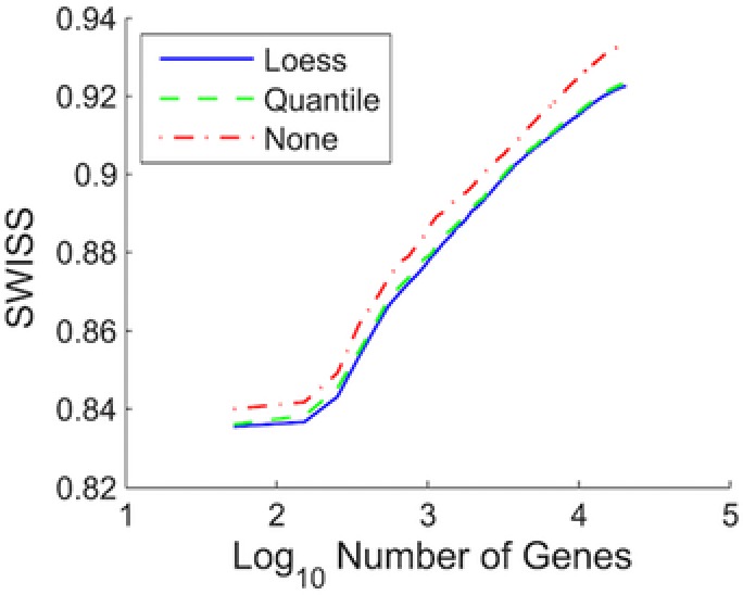
Normalization of a single channel design, data set II. Comparison of SWISS scores of three different normalization techniques for the single channel of data set II. The number of genes was varied, as shown by the x‐axis. Genes were filtered for each normalization method based on gene variation, keeping the genes with the largest variation. The normalization techniques being compared are loess (solid blue), quantile (dashed green), and no normalization (dot‐dashed red). This shows that for each fixed number of genes, quantile and loess normalization are both superior to no normalization, and that loess normalization performs slightly better than quantile normalization. This figure and legend were reproduced from ref. 9. Normalization of a single channel design, data set II. Comparison of SWISS scores of three different normalization techniques for the single channel of data set II: loess (solid blue), quantile (dashed green), and no normalization (dot‐dashed red).

The legend of Figure 4 contains all three critical elements:

1. An explanation of the graph elements (“The normalization techniques being compared are loess (solid blue), quantile (dashed green), and no normalization (dot‐dashed red).”);

2. A brief overview of the methods (“The number of genes was varied, as shown by the x‐axis. Genes were filtered for each normalization method based on gene variation, keeping the genes with the largest variation.”); and

3. A short summary of results (“This shows that for each fixed number of genes, quantile and loess normalization are both superior to no normalization, and that loess normalization performs slightly better than quantile normalization.”).

Without knowing anything about the SWISS score, the sentence summarizing results helps the audience understand that lower SWISS scores must be better because it states that quantile and loess normalization, which have lower SWISS scores, are both superior to no normalization.

Now compare the Figure 4 legend with this condensed version that is representative of most figure legends that appear in journal articles: Figure 4 : Normalization of a single channel design, data set II. Comparison of SWISS scores of three different normalization techniques for the single channel of data set II: loess (solid blue), quantile (dashed green), and no normalization (dot‐dashed red).

Notice how this condensed legend fails to provide a description of the methods and a summary of results. Which of the two figure legends do you find more informative?

PRINCIPLE 5: AVOID DECEPTION

“It is a capital mistake to theorize before one has data. Insensibly one begins to twist facts to suit theories, instead of theories to suit facts.” – Sherlock Holmes10

There are many ways that plots can be used to deceive an audience, whether intentional or not. This is especially important if you transform the data or axes, or only show summary statistics without the raw data.

Axis labels should always be appropriately scaled. When the goal is to compare data shown on two separate graphs, such as different subgroups, it is critical that the same scales are used for the axes on both graphs. For longitudinal data, time should be represented on a continuous scale, rather than a categorical scale, such as visit number, particularly when there may be different lengths of time between visits. You should also give careful consideration to including zero on each axis; if excluded, ensure its absence is clear. Finally, any transformations to the data or axes, such as square root or logarithmic transformations, should be clearly labeled both on the graph, in the legend, and when interpreting the results. This is especially critical when plotting lines on a transformed scale and concluding that there is a linear relationship or interpreting the slope. This was the sin that Purdue Pharma made in their figure of OxyContin drug levels: influencing health authorities and prescribers to believe that drug concentrations were relatively stable over time, but this was only true on the logarithmic scale and not on the linear scale.

Only displaying summary statistics or models, such as a least‐squares line, can be misleading, particularly if the model is wrong or somehow fundamentally flawed from the outset. You should make every effort to show the raw data. For example, Figure 5 displays nine data sets (a subset of the “Datasaurus Dozen”11) that have the same summary statistics (x and y mean, x and y SD, and correlation) to two decimal places of accuracy, while being drastically different in appearance.

Figure 5.

Nine data sets with equivalent summary statistics. Each data set has the same x mean (54.26), y mean (47.83), x SD (16.76), y SD (26.93), and Pearson correlation coefficient ( −0.06). The nine distinct patterns show the importance of plotting the raw data rather than only displaying summary statistics or models.

Displaying all data points instead of solely a summary statistic or model makes it easier to identify trends that are otherwise obvious, or are not well characterized by the model that was chosen, or are simply driven by outliers. We have observed numerous examples in which an apparent treatment effect is driven by a small number of outliers. Finding the appropriate summary statistic to account for outliers can be difficult but transparency is needed to tell the full story.

Including P values on a graph, either as text or symbols (such as *), can be misleading without context. Without this context, it is difficult for a graph to stand on its own. Examples of information that may be required include the test used to calculate the P values and whether the P values were adjusted for multiplicity. For journal articles, most of this detail can be provided in the Methods section, although the major highlights should be contained within the figure legend. For other medium, such as oral presentations, high‐level details should be provided alongside the graphic.

Colors, symbols, and line types should be easily distinguishable. When possible, try to use distinct colors rather than shades of a single color. Colors that are difficult to distinguish, that may not translate to gray scale, or that simply may not print well, such as certain yellows on white backgrounds, should also be avoided. It can also be helpful to use a colorblind‐friendly palette so that everyone in your audience can equally enjoy your graphics. Decisions around colorblind‐friendly palettes could include the selection of a red‐blue or blue‐green palette instead of a red‐green one. Preferred plotting symbols include the circle, square, triangle, plus (+), and “X.” It is important to ensure that the plotting symbols are large enough and the figure resolution is high enough that the different symbols can be distinguished. We recommend using as few line types as possible and instead to designate different groups by another medium, such as color. It is easy to distinguish between solid and a dashed line, but that distinction begins to become much more difficult when also adding dotted, dash‐dot, and other line types. Colors that are difficult to distinguish or those that may not print well, such as certain yellows, should also be avoided.

Occasionally, you may create a plot in which there is significant overlap in the data. This may occur when creating a scatterplot, or when you are plotting confidence intervals of two treatment groups for longitudinal data. In these instances, it may help to add some “jitter” to the points so that more of the data can be more easily seen. In other settings, alpha blending may also be a suitable alternative.

SUMMARY

We provided a set of five principles that will help you create the most informative data displays and provide greater clarity to your next journal article, grant proposal, or presentation.

Conflict of Interest

The authors declared no competing interests for this work.

References

- 1. Meier, B . Narcotic Maker Guilty of Deceit Over Marketing. The New York Times. May 11, 2007. A1 (2007).
- 2. Edwards, J . How Purdue Used Misleading Charts to Hide OxyContin's Addictive Power. CBS MoneyWatch [Internet]. https://www.cbsnews.com/news/how-purdue-used-misleading-charts-to-hide-oxycontins-addictive-power/ (2011). [Google Scholar]
- 3. Godin, S . Before you design a chart or infographic. Seth Godin. http://sethgodin.typepad.com/seths_blog/2018/01/before-you-design-a-chart-or-infographic.html. (2018). Accessed 15 January 2018.
- 4. Tufte, E . The Visual Display of Quantitative Information. (Graphics Press, Cheshire, CT, 1983).
- 5. Vale, R.D . Accelerating scientific publication in biology. Proc. Natl. Acad. Sci. USA 112, 13439–13446 (2015). [DOI] [PMC free article] [PubMed] [Google Scholar]
- 6. Kummu, M. , de Moel, H. , Ward, P.J. & Varis, O . How close do we live to water? A global analysis of population distance to freshwater bodies. PLoS One 6, e20578 (2011). [DOI] [PMC free article] [PubMed] [Google Scholar]
- 7. Stefaner, M . Talking with … Moritz Stefaner. Visualoop. http://visualoop.com/blog/19269/talking-with-moritz-stefaner. (2014). Accessed 15 January 2018.
- 8. Wiecki, T.V . et al A computational cognitive biomarker for early‐stage Huntington's disease. PLoS One 11, e0148409 (2016). [DOI] [PMC free article] [PubMed] [Google Scholar]
- 9. Cabanski, C.R . et al SWISS MADE: standardized within class sum of squares to evaluate methodologies and dataset elements. PLoS One 5, e9905 (2010). [DOI] [PMC free article] [PubMed] [Google Scholar]
- 10. Doyle, A.C. The Adventures of Sherlock Holmes. (George Newnes, London, UK, 1892).
- 11. Matejka, J. & Fitzmaurice, G. Same stats, different graphs: generating datasets with varied appearance and identical statistics through simulated annealing. Proceedings of the 2017 CHI Conference on Human Factors in Computing Systems, 1290–1294 (2017).