A multi-resolution approach for spinal metastasis detection using deep Siamese neural networks

Abstract

Spinal metastasis, a metastatic cancer of the spine, is the most common malignant disease in the spine. In this study, we investigate the feasibility of automated spinal metastasis detection in magnetic resonance imaging (MRI) by using deep learning methods. To accommodate the large variability in metastatic lesion sizes, we develop a Siamese deep neural network approach comprising three identical subnetworks for multi-resolution analysis and detection of spinal metastasis. At each location of interest, three image patches at three different resolutions are extracted and used as the input to the networks. To further reduce the false positives (FPs), we leverage the similarity between neighboring MRI slices, and adopt a weighted averaging strategy to aggregate the results obtained by the Siamese neural networks. The detection performance is evaluated on a set of 26 cases using a free-response receiver operating characteristic (FROC) analysis. The results show that the proposed approach correctly detects all the spinal metastatic lesions while producing only 0.40 FPs per case. At a true positive (TP) rate of 90%, the use of the aggregation reduces the FPs from 0.375 FPs per case to 0.207 FPs per case, a nearly 44.8% reduction. The results indicate that the proposed Siamese neural network method, combined with the aggregation strategy, provide a viable strategy for the automated detection of spinal metastasis in MRI images.

1. Introduction

Spinal metastasis, a metastatic cancer to the spine, is a malignant process in the spine. It is 25–35 times more common than any other malignant diseases in the spine [1] and affects more than 100,000 individuals in the U.S. annually [2]. The spine is the third most common site for cancer cells to metastasize [3], following the lung and the liver [4]. More than 80% of spinal metastasis in adults came from the primary tumors, including breast (72%), prostate (84%), lung (31%), thyroid (50%), kidney (37%), and pancreas (33%) [5]; and 30–90% of cancer patients who die are found to have spinal metastasis in cadaver studies [6]. In addition, spinal metastases can also have a huge impact on quality of life, with complications including pain, fracture, and spinal cord and nerve root compression [7]. Therefore, the detection, diagnosis, and treatment of spinal metastases are clinically important both to save patients’ lives and to improve their quality of life.

Due to its excellent soft tissue resolution, magnetic resonance imaging (MRI) is the most sensitive imaging modality for evaluating spinal lesions [8,9]. Various studies have shown that early stages of spinal metastasis in the bone marrow can be detected with MRI before any bone deterioration [5]. In MRI images, neoplastic involvement in the vertebral body typically shows focal bone marrow replacement with tumorous tissue, resulting in lower T1 signal than adjacent skeletal muscle and accompanying high T2 signal. Therefore, MRI images acquired with different pulse sequences (denoted as MRI sequences) can be used to locate lesions and evaluate the extent of the disease (e.g. involving single or multiple segments). However, despite the advantages mentioned above, the manual detection of spinal metastasis in MRI is time-consuming and tedious considering the large number of slices in each MRI sequence, as well as the large number of MRI sequences usually acquired for each patient. Therefore, it is now becoming essential to develop computerized algorithms for automated detection of spinal metastases in MRI sequences.

Especially, as image acquisition speed improves, many more images with a higher spatial resolution can be acquired during an examination, and as such developing computer-aided analysis methods is essential to assist radiologists in making a thorough evaluation of the entire image set within a reasonable reading time. This is a trend for all imaging modalities (and all pathologies), and particularly true for MRI because of the multiple sets of images acquired using different sequences. Although at the present time computer-aided analysis cannot yet replace visual inspection by trained radiologists, nonetheless it can already provide an important tool for displaying the most critical information from hundreds of images, in a convenient way, to assist radiologists during diagnosis. In time, computerized methods may become as good, or even better than human experts and lead to significant economies of scale and accuracy. Thus, in short, it is important to develop computerized methods to analyze MRI and other imaging modalities in medicine.

Given the importance of automated spinal metastasis detection, a few approaches have been developed in the literature. For example, Roth et al. [10] used a deep convolutional neural network (CNN) as the 2nd tier of a two-tiered, coarse-to-fine, cascade framework to refine the candidate lesions from the first tier for sclerotic spine metastasis detection in computer tomography (CT) images. Wiese et al. [11] developed an automatic method based on a watershed algorithm and graph cut for detecting sclerotic spine metastases in CT images. And Yao et al. [12] applied a support vector machine to refine the initial detections produced with a watershed algorithm for lytic bone metastasis detection in CT images. However, as can be seen, these studies are based on CT images and do not use spinal MRI sequences.

On the MRI side, efforts for analyzing MRI sequences have focused on different problems. For example, Carballido-Gamio et al. [13] developed a normalized cut method for vertebra segmentation in spinal MRI. Huang et al. [14] proposed an AdaBoost method for vertebra detection and an iterative normalized cut algorithm for vertebra segmentation in spinal MRI. Neubert et al. [15] designed an automatic method using statistical shape analysis and registration of gray level intensity profiles for 3D intervertebral disc and vertebral body segmentation in MRI. However, in spite of these efforts and to the best of our knowledge, there is no study in the literature that is focused on detecting spinal metastases in MRI sequences.

Automated and accurate spinal metastasis detection in MRI is a difficult task, in large part because of the considerable variability in the size of vertebrae. Spinal metastases usually grow in the vertebrae, which are divided into five regions: cervical, thoracic, lumbar, sacrum, and coccyx. The size of the vertebrae varies considerably both within an individual, as well as across individuals. For example, Zhou et al. [16] investigated the lumbar vertebrae from 126 CT images and found that the upper vertebral width is 40.9 ± 3.6 mm in females and 46.1 ± 3.2 mm in males at L3, 46.7 ± 4.7 mm in females and 50.8 ± 3.7 mm in males at L4, and 50.4 ± 4.4 mm in females and 54.5 ± 4.9 mm in males at L5.

In recent years [17], neural networks and deep learning have been used to successfully tackle a variety of problems in engineering, ranging from computer vision [18–20] to speech recognition [21], as well as in the natural sciences, in areas ranging from high energy physics [22,23], to chemistry [24,25], and to biology [26,27]. Thus it is natural to consider applying deep learning methods also to biomedical images. For example, Ciresan et al. applied a deep learning architecture to each pixel for addressing problems of membrane segmentation in electron microscopy images [28]; Shen et al. developed multi-scale convolutional neural network for lung nodule detection in CT images [29]; Wang et al. adopted a GoogLeNet-based method for automated detection and diagnosis of metastatic breast cancer in whole slide images of sentinel lymph node biopsies [30]; and Wang et al. devised a 12-layer convolutional neural network for cardiovascular disease detection in mammograms [31]. Therefore it is natural to hypothesize that neural networks and deep learning methods can be harnessed for the effective detection of spinal metastases in MRI sequences.

Thus, in short, the purpose of this study is to develop an accurate computerized method to locate metastatic cancer in the spine using deep learning methods. Specifically, a multi-resolution analysis is proposed to deal with the large variability of vertebral sizes, and a Siamese neural network [32,33] is developed to incorporate the multi-resolution representation of each MRI slice. More precisely, for each location under consideration, a set of image patches centered at this location and at different resolutions are extracted from the MRI slice, resulting in a multi-resolution representation of the input. Then the multi-resolution image patches are fed into a Siamese neural network to predict the probability that the corresponding location corresponds to a metastatic lesion. The Siamese neural network is composed of several identical networks, each dealing with patches of a different resolution. To further remove false positives (FPs) in spinal metastasis detection, we consider the structural similarity of neighboring slices in MRI sequences and aggregate the outputs of the Siamese neural networks using a weighted averaging approach.

The rest of paper is organized as follows. The proposed Siamese neural network and slice-based aggregation methods for spinal metastasis detection are descried in Section 2 together with other methodological aspects. The data collection and experiments are described in Section 3. Finally, the results are presented in Section 4 and discussed in Section 5.

2. Methods

2.1. Motivation

As previously mentioned in Section 1, there is considerable variability in vertebral size. Such variability results in great variations in the sizes of the metastatic lesions, thus yielding the difficulty in the metastatic lesion detection. In Fig. 1, we provide examples of metastatic lesions with different sizes, in which each image window represents a region of 55 × 79 mm². As can be seen, the size of the metastatic lesion varies hugely, in which the first lesions cover almost 55 mm in width, while the last lesions only has less than half of 55 mm in width.

Fig. 1.

Example of the variability of the lesion size. Each image window represents a region of 55 × 79 mm².

In real application, such variability as mentioned above poses a major challenge for metastatic lesion detection. This is because most detectors (if not all) are usually designed to examine only a relatively small image patch around the location under consideration. Having local detectors can be computationally efficient. However, in our case, if the local image patch is too small and the vertebra is large, then the detector sees only a fraction of the vertebra and cannot accurately distinguish between lesion and normal. In contrast, if the local image patch is big and the vertebra is small, then most of the information contained in the patch is not relevant for the discrimination. Therefore, to accommodate for large variations in vertebral size, we propose a multi-resolution approach for spinal metastasis detection. Specifically, for each location of interest, we extract three image patches with same size in pixels from each MRI slice, corresponding to three different resolutions, yielding three different local representations of the location under consideration. The goal is to make sure that when metastatic lesions are present, they are salient in at least two image patches. Furthermore, in order to control the number of parameters and regularize the overall model, we use the same parameters in the networks associated with each resolution.

More precisely, to incorporate the input of the three image patches into a unified classification framework, we use a Siamese neural network. The Siamese neural network consists of three identical subnetworks, one for each image patch. Each subnetwork is a multilayer convolutional neural network, where the lower convolutional layers are used to learn and extract features which in turn are used to produce a classification by several the higher, fully connected (FC) layers. The output of the Siamese neural network can be interpreted as the probability of a metastatic lesion being associated with the central pixel in the input patch. The advantages of such an architecture are the ability to automatically learn and extract relevant features, and the combination of multi-resolution features for classification. In addition, by the Siamese neural network design, the three subnetworks share the same weight parameters. Thus the number of trainable parameters remains manageable and independent of the number of resolution patches.

2.2. Siamese neural network architecture

The subnetworks of the overall Siamese architecture comprise stacks of convolutional layers (Conv), batch normalization layers, nonlinearity layers, and max-pooling layers (Pooling). Each convolutional layer is followed by a batch normalization layer and a non-linear transformation. The convolutional layers are feature extractors, and the max-pooling layers enable the combination of low-level features into high-level features. In Fig. 2, we display the Siamese neural network architecture used in this study. Each subnetwork includes five convolutional layers. To avoid cluttering the figure, the batch normalization layer and the non-linearity layer, associated with each convolutional layer, are not shown. Finally, the features learned by the subnetworks are concatenated and fed into two fully connected layers for the final classification. The details of each layer are as follows.

Fig. 2.

Diagram of the Siamese architecture used in this study. There are three identical subnetworks, each comprising five convolutional layers, five batch normalization layers, five nonlinearity layers, and four max-pooling layers for feature learning. The combination of the resulting features is subsequently input into two fully connected layers for classification. Each convolutional layer is followed by a batch normalization layer and a nonlinearity layer (not shown).

In the development phase, we experimented with subnetworks by using many other architectures and in Fig. 2 we only report the one with the best performance. The architecture of the subnetworks has a sequence of 1, 2, and 2 convolutional layers before the first three max-pooling layers, respectively. In one experiment, for instance, we started from an architecture with a sequence of 1, 1, and 1 convolutional layers for subnetworks, and then we gradually increased the number of convolutional layers and stopped when no further improvement was observed.

Convolutional layers are the core layers for feature learning and extraction. Each convolutional layer produces a feature map by convolving its input with a set of convolutional kernels. Mathematically, let x be the input, y_k be the kth feature map in output, and w_k (k = 1, 2, …, K, where K is the number of convolutional kernels) be the kth convolutional kernel, then the convolutional layer can be described by:

$${\mathbf{y}}_k=\mathbf{x}\ast {\mathbf{w}}_k+b_k$$ (1)

where * denotes the convolution operation and b_k is the bias. Usually, there are several convolutional kernels in each convolutional layer (i.e. K > 1). In Fig. 2, the number of convolutional kernels corresponds to the number preceding the symbol “@” in the line at the top. For example, 16 convolutional kernels are used in the first convolutional layer in Fig. 2. In this study, the size of all of the convolutional kernels is set as 3×3.

Batch normalization layers independently normalize the feature values to zero mean and unit standard deviation in each training batch. These are introduced to deal with the internal covariate shift, which refers to the phenomenon that the distribution of each layer’s inputs changes during training when the parameters of the previous layers change [34]. This normalization step can speed up learning and improve classification accuracy [34]. Batch normalization layers preserve both the number and the size of the feature maps; to save space, they are omitted in Fig. 2.

Nonlinearity layers consist of units which apply a non-linear activation function to their input, producing in the end a non-linear classifier. In this study, we use rectified linear units (ReLU), with a non-linear activation function:

$$f(x)=max(0,x)$$ (2)

While similar results could be obtained with sigmoidal transfer functions, ReLU units can lead to faster training [18,35] and yield sparse representations [35]. Just like the batch normalization layers, the nonlinearity layers also preserve both the number and the size of the feature maps; to save space, they are omitted in Fig. 2.

Max-pooling layers serve as a method of non-linear down-sampling, by providing a summary of the outputs of a set of neighboring elements in the corresponding feature maps, simply by retaining the maximum value of the elements in each pool [36]. In this study, two types of max-pooling layers are considered. The first type of max-pooling layer generates its output by considering the 3×3 neighborhood region of the same feature map, thus reducing the size of the feature maps by nearly 50%; the second type of max-pooling layer produces its output by considering a feature map and its next feature map at the same location, thus reducing the number of feature maps by half. In this study, the first type is used for the first three max-pooling layers, and the second type is used for the last max-pooling layer. In Fig. 2, the size of the feature maps is displayed in the top line, right after the “@” sign. By comparing the number and size of the feature maps between the input and the output at each stage, one can determine the type of max-pooling layer in Fig. 2. For example, it can be seen that for the first max-pooling layer, the number of feature maps does not change from input to output, but the size of the feature maps decreased from 55×79 to 27×39, thus it is the first type of max-pooling layer.

Fully connected layers correspond to pairs of consecutive layers with full connectivity between their units. The input of the first fully connected layers is concatenation of all of the features from the three subnetworks.

After the last fully connected layer, a softmax activation function [19] is introduced, the output of which can be interpreted as the probability that the central pixel in the input image patch is associated with a metastatic lesion.

2.3. Model training

In total, the Siamese neural network in Fig. 2 has around 733.4K trainable parameters. The parameters are learnt by stochastic gradient descent in order to minimize the cross entropy between true class labels and predicted outputs, together with standard L2 regularization. Let (x_i, y_i), i = 1, 2, …, M (M is the number of training samples) be the input and true label training pairs, and p_i the corresponding predicted output for input x_i, then the objective function can written as:

$$J(\mathbf{w})=-\sum _{i=1}^m[y_{i}log{p}_i+(1-y_i)log(1-p_i)]+\lambda {\Vert \mathbf{w}\Vert }_2^2$$ (3)

where w denotes all the weight parameters in the model and λ is a constant which controls the trade-off between the classification error on the training samples and the complexity of the model.

To further reduce the potential for overfitting, we use dropout [37,38], which can be viewed as a regularization technique. Dropout randomly drops neural units during training to prevent any unit from being too reliant on any other unit (unit co-adaptation). In this study, dropout with probability 0.5 is applied to the first fully connected layer.

2.4. Training samples extraction

As input to the proposed Siamese neural network architecture, we choose image patches with size of 55×79 pixels from the MRI slices at three different resolutions, i.e. 0.5 mm/pixel, 1 mm/pixel, and 2 mm/pixel, as shown for the input layers in Fig. 2. Such choice ensures that at least two out of the three image patches cover more than one vertebra. It is based on two observations: (1) vertebrae have roughly a square shape, and the width of the majority of the lumbar vertebrae is in the range of 37.3–59.4 mm [16]; and (2) during the diagnostic process, radiologists usually compare the vertebra under consideration with other vertebrae in the same MRI slice. More importantly, when single image resolution is considered, the image patch size 55×79 achieves the best detection performance at the resolution of 1 mm/pixel.

As examples, in the first column of Fig. 3(a), we show the multi-resolution image patches from a big metastatic lesion. The image resolutions for the image patches in the first, second, and third rows are 0.5 mm/pixel, 1 mm/pixel and 2 mm/pixel, respectively. As can be seen, the metastatic lesion is salient in the image patches with resolutions of 1 mm/pixel and 2 mm/pixel. Similarly, in the first column of Fig. 3(b), we also show the multi-resolution image patches from a small metastatic lesion. It can be seen that the metastatic lesion is salient in the image patches with resolutions of 1 mm/pixel and 0.5 mm/pixel.

Fig. 3.

Examples of multi-resolution image patches from a big metastatic lesion (a) and those from a small metastatic lesion (b). The resolutions of the image patches from the first to the third rows are 0.5 mm/pixel, 1 mm/pixel, and 2 mm/pixel. In each image patch, the boundary of the metastatic lesion is marked by a red contour. For demonstration purposes, the image patches after data augmentation are shown as well. (For interpretation of the references to color in this figure caption, the reader is referred to the web version of this paper.)

The training of the Siamese neural network requires a large number of training samples. For this purpose, we extracted training samples from the MRI sequences in the training set, described in Section 3.1, as follows: for an MRI slice under consideration, to maximize the number of metastatic lesion samples, we extract image patches from each pixel in the spinal metastatic region. Then to obtain corresponding normal samples, we randomly extract the same number of image patches from the normal region in the slice, to prevent imbalance between the two classes. To reduce the variation among the samples, a z-score normalization is applied to each image patch such that each component has zero mean and unit standard deviation.

Note the samples associated with the normal class mainly include two types of samples, the ones from the normal vertebral regions, and the ones from the non-vertebral background regions. For spinal metastasis detection, it is much more difficult to discriminate between metastatic lesions and normal vertebrae than to discriminate between metastatic lesions and background. For this reason, we select more normal samples from the normal vertebral regions. In this study, 70% of the normal samples are randomly selected from the normal vertebral regions, while the remaining 30% normal samples are randomly selected from the background regions.

In Fig. 4, we show an MRI slice and its spinal metastatic region marked by a radiologist with a red contour together with vertebral regions marked with blue contours. Specially, for this MRI slice, all of the spinal metastasis samples are extracted from the region indicated by the red contour, 70% of normal samples are extracted from the region outside the red contour but inside the blue contours, and 30% of normal samples are extracted from the region outside the blue and red contours. It has to be noted that both the spinal metastatic and vertebral regions are only used for sample extraction, they are unknown at test time.

Fig. 4.

Example of lesion region, denoted by the red contour, and vertebral region, denoted by the blue contour in an MRI slice. (For interpretation of the references to color in this figure caption, the reader is referred to the web version of this paper.)

Finally, to increase the number of training samples, we use a data augmentation strategy. Data augmentation has been shown to be effective in many cases [18,39]. To preserve the resolution of the image patches, we consider the following two data augmentation strategies for the samples in the training set: (1) flipping image windows from left to right and (2) flipping image windows from top to bottom. In combinations, these strategies can lead to a four-fold increase in the size of the training set. Examples of augmented data are shown in the second to fourth columns of Fig. 3 for two representative metastatic lesions.

2.5. Testing

2.5.1. Likelihood map

During testing, the trained model is applied to each pixel of an MRI slice in the testing set. The output is a likelihood map, denoted by l, with the same size as the MRI slice under consideration. The value of each pixel in the likelihood map is the estimated probability, according to the network, that the pixel corresponds to a metastatic lesion. When the locations are close to the boundary of the slice, the image patches extend beyond the slice boundaries and symmetric padding is used to fill any region of the patches falling outside the boundaries.

2.5.2. Slice-based aggregation

Spinal metastases can be recovered by processing the likelihood map of each MRI slice and finding regions of high probability. However, using a single likelihood map tends to yield many FPs when all the true positives (TPs) are detected. To further reduce the number of FPs, we take advantage of the 3D information associated with MRI sequence and generate an aggregated likelihood map, denoted by L, for each slice.

Examination of MRI sequences reveals that slice may vary greatly but neighboring slices tend to be very similar. Based on this observation, for the ith slice and location (x, y) in an MRI sequence, we generate an aggregated likelihood using a weighted convex combination as follows:

$$L_i(x,y)=\sum _{j\in \mathcal{N}(i)}{\alpha }_j{l}_j(x,y)$$ (4)

where 𝒩(i) denotes the neighboring slices of the ith slice and α_j is the weight of the jth slice. The weights must be positive and satisfy Σ_j∈𝒩(i) α_j = 1 and α_i > α_j, j ≠ i. The constraint α_i > α_j, j ≠ i, indicates that when obtaining the aggregated likelihood map for the ith slice, more emphasis should be put on its likelihood map l_i as compared to the likelihood maps l_j of its neighbors. In this study, for a slice under consideration, we consider its previous and next slices as neighboring slices used for aggregation. When the slice is the first or last slice in the MRI sequence, its next two slices or previous two slices are considered as its neighboring slices. In the experiments, we considered identical weights for both of the neighboring slices. We did a grid search on the weights of the slice on the values 1/3, 0.4, 0.5, and 0.6. In the end, the best performance was obtained at 0.4, thus the weight of the slice and its two neighboring slices were set to be 0.4, 0.3, and 0.3 respectively.

Finally, a threshold is applied to the aggregated likelihood map for spinal metastasis detection. To further reduce the number of FPs, detected regions of size smaller than 5 cm² are considered to be FPs and are removed from the list of positives. The use of 5 cm² is based on two observations: (1) the average abnormal segment area in the dataset is 5.07 cm², as described in Section 3.1 and (2) the proposed method tends to produce detected regions that are larger than those marked by radiologists, as shown in Figs. 6 and 8.

Fig. 6.

Examples of three consecutive slices in an MRI sequence (top) and their corresponding aggregated likelihood maps (bottom). The spinal metastasis boundaries provided by the radiologist are marked by red contours, while the boundaries of the detections obtained with a threshold of 0.6 are marked by blue contours. (For interpretation of the references to color in this figure caption, the reader is referred to the web version of this paper.)

Fig. 8.

Example of three consecutive slices in an MRI sequence (top) and their corresponding aggregated likelihood maps (below). The spinal metastasis boundaries provided by the radiologist are marked by red contours, while the boundaries of the detections obtained with a threshold of 0.6 are marked by blue contours. In this case, there is a false-positive contour in the right slide associated with the cerebellum. (For interpretation of the references to color in this figure caption, the reader is referred to the web version of this paper.)

3. Experiments

3.1. Dataset

In this study we made use of sagittal MRI images of the spines from 26 cases, including 14 males and 12 females, with an age range of 58 ± 14 years (mean ± standard deviation). They were obtained from the clinical database of the Peking University Third Hospital. MR scans were performed on a 3.0 T Siemens Trio scanner. Only the set of sagittal images acquired by using the fat-suppressed T2-weighted inversion recovery pulse sequence, in which the metastatic cancer was most clearly visible, was analyzed. The imaging parameters were: TR=4780 ms, TE=64 ms, TI=200 ms, Echo Train length=9, Field of View=340 mm × 340 mm, slice thickness=3 mm. The resolution of the images is 0.88 mm/pixel, 0.94 mm/pixel, or 1.13 mm/pixel.

In this dataset, the primary cancers were 15 lung, 5 thyroid, two liver, one breast, one prostate, one esophagus, one urinary tract. All patients were symptomatic with spinal pain but without any known cause; thus they were referred for diagnosis by MRI. Biopsies were subsequently taken from all patients and the diagnosis of metastatic cancer was confirmed through pathological examination of all biopsy specimens. For this initial study, all the cases under consideration were carefully selected based on confined disease in only one or two vertebral body segments. Among these cases, the area of the smallest abnormal segment was 1.65 cm², the area of the largest abnormal segment was 9.54 cm², and the average area of the abnormal segments was 5.07 cm².

The metastatic lesions in each MRI slice were identified and manually traced by an experienced radiologist, and the boundary of the vertebral bodies was marked manually by two of the authors of this study. In each case there are a total of 13 sagittal images covering the entire spine and, depending on the size of the lesion, the radiologist selected 3–7 slices that contained the lesion and manually outlined the metastatic lesions.

To facilitate the spinal metastasis detection, all the MRI slices are transformed into resolutions of 0.5 mm/pixel, 1 mm/pixel, and 2 mm/pixel for multi-resolution analysis. In the development phase, we also considered the multi-resolution analysis in the resolutions of 0.25 mm/pixel, 1 mm/pixel, and 1.25 mm/pixel and the resolutions of 0.5 mm/pixel, 1 mm/pixel, and 1.5 pixel, but got worse detection performance. The detection performance is evaluated at the resolution of 1 mm/pixel. To speed up the spinal metastasis detection, only the half center of the MRI slices along the x-axis of the images, containing the vertebral bodies, are considered [13].

3.2. Experimental setup

In our experiments, to get an overall evaluation performance for the whole dataset, we applied a case-based 10-fold cross-validation procedure as follows. The dataset was first randomly divided into 10 equally sized subsets; in each run, a subset is hold out for performance evaluation (i.e. “testing subset”) and the remaining data is randomly partitioned into two subsets, one containing 75% of the examples for training (i.e. “training subset”) and the other containing 25% of the examples for validation (i.e. “validation subset”). To avoid any potential bias, the MRI slices from one case were always assigned together to either the training subset, or the validation subset, or the testing subset, but never spread across multiple subsets.

The Siamese neural network model was implemented by a Theano-based deep learning framework – Lasagne. It was trained by stochastic gradient descent (SGD) [40], with a batch size of 128, momentum of 0.9, and learning rate of 0.06. On average, there were 85,503 training examples in each run based on the sample extraction procedure described in Section 2.4.

λ in (3) is an important parameter for controlling model complexity and the risk of overfitting during training. To determine the optimal parameter λ, a grid search procedure was considered by evaluating the classification error on the samples in the validation set. Values of 0.001, 0.01, and 0.1 were considered for λ in the grid search and a value of 0.01 is used in the final system. To obtain the samples for validation, the sample extraction procedure described in Section 2.4 was applied to the MRI slices in the validation set (described in Section 3.1).

3.3. Performance evaluation

For performance evaluation, we conduct a free-response receiver operating characteristic (FROC) analysis on the detection results. FROC analysis is widely used for detection performance evaluation in medical imaging [10,41], and it provides an overall spinal metastasis detection performance evaluation with respect to the ground truth provided by the radiologists across all possible decision thresholds. In particular, we compute and plot the FROC curve corresponding to the true-positive (TP) rate on the y-axis versus the number of FPs per case on the x-axis, in which the TP rate is calculated as the ratio of the number of TPs over the number of true spinal metastatic regions.

Very often we find cases where the cancer has spread outside the vertebrae resulting in soft tissue lesions with similar signal intensity as the cancer lesions inside the vertebrae. In this case, the automatic detection method developed in this work would segment the entire lesion, both inside and outside the vertebrae. Therefore, in the FROC analysis, a detection is considered to be a TP if its center of gravity falls within 20 mm from the center of gravity of the region outlined by the radiologist; otherwise, it is considered to be a FP.

While the spinal metastasis detection is conducted for each MRI slice, the FROC analysis is done on a per-case basis as follows. For each case, its TP rate and the number of FPs is obtained as the average of the TP rate and the average of the number of FPs, computed over the corresponding MRI sequence. For each MRI sequence, its TP rate and the number of FPs are obtained by averaging the TP rate and the number of FPs of all its slices. The purpose of such case-based FROC analysis is to accommodate for the fact that it is the same lesions that are under evaluation for the different slices of the different MRI sequences associated with a given case. The case-based analysis is used in general to avoid any potential bias introduced by differences in the number of MRI slices and MRI sequences, although in this particular study, only one MRI sequence is available for each case.

To accommodate for the variations associated with the distribution of the cases and to facilitate statistical comparison, we apply a bootstrapping procedure in the FROC analysis [41]. In our experiments, a total of 20,000 bootstrap samples were used, based on which the p-value was reported on the detection results.

4. Results

In Fig. 5, we show the FROC curve obtained by the proposed approach, both with and without the aggregation procedure for comparison purpose. As can be seen, the FROC curve is noticeably improved when information from neighboring slides is aggregated. A statistical comparison between the proposed approach with and without the use of aggregation yields p-value of 0.0014 for FPs over the range of [0, 0.5] per case. Specifically, at TP rate of 90%, the FP rate is reduced from 0.375 per case without aggregation to 0.207 per case with aggregation, nearly a 44.8% reduction. Moreover, with a FP rate of 0.20 per case, the sensitivity is improved from 72.7% without aggregation to 89.1% with aggregation. Finally, it can be seen that the proposed approach yields only 0.40 FPs per case when correctly detecting all the spinal metastasis.

Fig. 5.

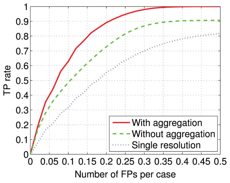
The detection performance achieved by the proposed approach (with aggregation). To demonstrate the effectiveness of the aggregation, the detection performance without the use of the aggregation is shown for comparison (without aggregation). To demonstrate the effectiveness of the multi-resolution method, the detection performance achieved by using only one resolution (i.e. 1 mm/pixel) is shown as well.

In Fig. 6, we show an example of three consecutive slices from an MRI sequence (top) and their corresponding aggregated likelihood maps (bottom). To demonstrate the corresponding detections, we apply a threshold of 0.6, and the detection boundaries are marked by blue contours. For comparison purposes, the boundaries of the metastatic lesions provided by the radiologist are marked by red contours. As can be seen, the proposed approach using the aggregated likelihood map correctly detects all the metastatic lesions.

For comparison, in Fig. 7, we show the same example of three consecutive slices, as in Fig. 6 (top) and the corresponding likelihood maps without using the aggregation strategy (bottom). As in Fig. 6, the boundaries of the metastatic lesions provided by the radiologist are marked by red contours, while the boundaries of the regions detected using a threshold of 0.6 are marked by blue contours. Compared with Fig. 6, one FP contour appears in the middle slice, clearly exemplifying how the aggregation procedure can indeed reduce the FP rate in spinal metastasis detection.

Fig. 7.

Example of three consecutive slices in an MRI sequence (top) and their corresponding likelihood maps without the use of aggregation (bottom). The spinal metastasis boundaries provided by the radiologist are marked by red contours, while the boundaries of the detections obtained with a threshold of 0.6 are marked by blue contours. In this case, the lack of aggregation results in the false-positive blue contour detection in the middle slide. (For interpretation of the references to color in this figure caption, the reader is referred to the web version of this paper.)

Finally, to demonstrate the effectiveness of the multi-resolution approach, in Fig. 5, for comparison purposes, we also show the best detection performance achieved by the single resolution method, using the patch size 55×79 at image resolution 1 mm/pixel. The slice-based aggregation method was applied as well. As can be seen, the FROC curve of the proposed multi-resolution approach is noticeably higher than the single resolution method. A statistical comparison between them yields p-value of 0.0083 for FPs over the range of [0, 0.5] per case. Specifically, with a FP rate of 0.20 per case, the sensitivity is improved from 55.4% for single resolution method to 89.1% for multi-resolution approach.

5. Discussion

5.1. FP analysis

To better understand the occurrence of FPs in spinal metastasis detection, in Fig. 8 we show another example of three consecutive slices from an MRI sequence (top) and the corresponding aggregated likelihood maps (bottom). In these plots, the boundaries of the spinal metastatic lesions provided by the radiologist are marked by red contours, while the boundaries of the regions detected using a threshold of 0.6 are marked by blue contours. As can be seen, there is one FP contour in the right slice of Fig. 8. This FP corresponds to the cerebellum which typically has a moderate T2 signal intensity similar to that of a spinal lesion. Based on this example, we manually examined all the FPs detected at a threshold of 0.6, and found that most FPs (6 out of 8 cases) occur in the cerebellum. Such FPs which have nothing to do with the spine can easily be removed if an algorithm for vertebral region detection is applied before spinal metastasis detection. Indeed, we found that only one FP in one slice of one MRI sequence happens at the vertebral region, indicating that the proposed approach is indeed accurate in spinal metastasis detection.

5.2. Limitations

The results from this study indicate that the proposed approach can detect spinal metastasis in MRI accurately. It has to be noted that all the cases considered in this study contain metastatic lesions. In the future, it might be desirable to include some normal cases (i.e. cases without metastatic lesions) as well. However, we note that in our dataset, the majority of local regions in the MRI sequences do not have any metastatic lesions, thus can be viewed as substitutes for normal cases in terms of FP detection. Therefore, the reported number of FPs per case will likely remain very similar when normal cases are included. Nevertheless, the inclusion of normal cases should be helpful for more comprehensive evaluations, in particular for estimating positive predictive values (PPV) and negative predictive values (NPV) in image screening.

The dataset used in this study consisted of only 26 cases. Although it is labor intensive, it would be obviously desirable in the future to curate larger data sets, containing more cases, to evaluate the proposed method more comprehensively. Furthermore, having larger training sets may also allow one to train more accurate Siamese networks with similar, or even more complex, architectures which may ultimately improve detection performance.

From the results in Section 4, the proposed method can accurately detect spinal metastases in MRI sequences. However, from Figs. 6 to 8, it can be seen that the boundaries of the regions detected by the proposed approach tend to be less accurate. Nevertheless, if the need were to arise in applications for accurate metastatic boundary segmentation, any semi-automatic segmentation method – such as level set segmentation [42] or active contour model [43,44] – could be included, as a post-processing step for refining the segmentation of the spinal metastatic lesions. These segmentation methods would benefit from the initialization of seed points provided by the proposed approach. It must be noted, however, that the development and evaluation of accurate segmentation methods would face even greater data challenges, as not only it would require more curated data, but also the curation process itself would pose great challenges (e.g. a reader study). This is because different radiologists may easily agree on the presence or absence of a lesion but, when present, may disagree on its precise boundaries.

6. Conclusion

In this study, we have investigated the feasibility of automatic spinal metastasis detection in MRI by using deep learning methods. For this purpose, we developed and implemented a multi-resolution approach using a Siamese convolutional neural network to accommodate for the large variability in vertebral body size. The output of the Siamese neural network is further aggregated across neighboring slices in an MRI sequence to further reduce the FP rate. We have evaluated the detection performance on a set of 26 cases by FROC analysis. The results show that the proposed approach is effective and can correctly detect all the spinal metastatic lesions while obtaining only 0.40 FPs per case. At TP rate of 90%, the use of the aggregation reduces the FPs from 0.375 FPs per case to 0.207 FPs per case, a nearly 44.8% reduction. Taken together, these results show that the proposed Siamese neural network with the aggregation strategy has the potential for providing the basis for an automated accurate spinal metastasis detection system that can be clinically deployed. The approach and its evaluation will greatly benefit in the future from the aggregation and curation of larger datasets.

References

- 1.Mundy GR. Metastasis to bone: causes, consequences and therapeutic opportunities. Nat Rev Cancer. 2002;2(8):584–593. doi: 10.1038/nrc867. [DOI] [PubMed] [Google Scholar]
- 2.Murphy MJ, Chang S, Gibbs I, Le QT, Martin D, Kim D. Image-guided radiosurgery in the treatment of spinal metastases. Neurosurg Focus. 2001;11(6):1–7. doi: 10.3171/foc.2001.11.6.7. [DOI] [PubMed] [Google Scholar]
- 3.Witham TF, Khavkin YA, Gallia GL, Wolinsky JP, Gokaslan ZL. Surgery insight: current management of epidural spinal cord compression from metastatic spine disease. Nat Clin Pract Neurol. 2006;2(2):87–94. doi: 10.1038/ncpneuro0116. [DOI] [PubMed] [Google Scholar]
- 4.Klimo P, Schmidt MH. Surgical management of spinal metastases. Oncologist. 2004;9(2):188–196. doi: 10.1634/theoncologist.9-2-188. [DOI] [PubMed] [Google Scholar]
- 5.Shah LM, Salzman KL. Imaging of spinal metastatic disease. Int J Surg Oncol. 2011 doi: 10.1155/2011/769753. [DOI] [PMC free article] [PubMed] [Google Scholar]
- 6.Sciubba DM, Petteys RJ, Dekutoski MB, Fisher CG, Fehlings MG, Ondra SL, Rhines LD, Gokaslan ZL. Diagnosis and management of metastatic spine disease: a review. J Neurosurg: Spine. 2010;13(1):94–108. doi: 10.3171/2010.3.SPINE09202. [DOI] [PubMed] [Google Scholar]
- 7.Pope T, Bloem HL, Beltran J, Morrison WB, Wilson DJ. Musculoskeletal Imaging. Elsevier Health Sciences; Philadelphia, US: 2014. [Google Scholar]
- 8.Algra PR, Bloem JL, Tissing H, Falke T, Arndt J, Verboom L. Detection of vertebral metastases: comparison between MR imaging and bone scintigraphy. Radiographics. 1991;11(2):219–232. doi: 10.1148/radiographics.11.2.2028061. [DOI] [PubMed] [Google Scholar]
- 9.O’Sullivan GJ, Carty FL, Cronin CG. Imaging of bone metastasis: an update. World J Radiol. 2015;7(8):202. doi: 10.4329/wjr.v7.i8.202. [DOI] [PMC free article] [PubMed] [Google Scholar]
- 10.Roth HR, Yao J, Lu L, Stieger J, Burns JE, Summers RM. Recent Advances in Computational Methods and Clinical Applications for Spine Imaging. Springer International Publishing; Switzerland: 2015. Detection of sclerotic spine metastases via random aggregation of deep convolutional neural network classifications; pp. 3–12. [Google Scholar]
- 11.Wiese T, Yao J, Burns JE, Summers RM. Detection of sclerotic bone metastases in the spine using watershed algorithm and graph cut. SPIE Medical Imaging, International Society for Optics and Photonics, Medical Imaging: Computer-Aided Diagnosis; San Diego, CA, USA. 2012; p. 831512. [Google Scholar]
- 12.Yao J, O’Connor SD, Summers R. Computer aided lytic bone metastasis detection using regular CT images. Medical Imaging, International Society for Optics and Photonics, Medical Imaging: Image Processing; San Diego, CA, USA. 2006; p. 614459. [Google Scholar]
- 13.Carballido-Gamio J, Belongie SJ, Majumdar S. Normalized cuts in 3-d for spinal MRI segmentation. IEEE Trans Med Imaging. 2004;23(1):36–44. doi: 10.1109/TMI.2003.819929. [DOI] [PubMed] [Google Scholar]
- 14.Huang SH, Chu YH, Lai SH, Novak CL. Learning-based vertebra detection and iterative normalized-cut segmentation for spinal mri. IEEE Trans Med Imaging. 2009;28(10):1595–1605. doi: 10.1109/TMI.2009.2023362. [DOI] [PubMed] [Google Scholar]
- 15.Neubert A, Fripp J, Engstrom C, Schwarz R, Lauer L, Salvado O, Crozier S. Automated detection, 3D segmentation and analysis of high resolution spine MR images using statistical shape models. Phys Med Biol. 2012;57(24):8357. doi: 10.1088/0031-9155/57/24/8357. [DOI] [PubMed] [Google Scholar]
- 16.Zhou SH, Mccarthy ID, Mcgregor AH, Coombs RR, Hughes SP. Geometrical dimensions of the lower lumbar vertebrae – analysis of data from digitised CT images. Eur Spine J. 2000;9(3):242–248. doi: 10.1007/s005860000140. [DOI] [PMC free article] [PubMed] [Google Scholar]
- 17.Schmidhuber J. Deep learning in neural networks: an overview. Neural Netw. 2015;61:85–117. doi: 10.1016/j.neunet.2014.09.003. [DOI] [PubMed] [Google Scholar]
- 18.Krizhevsky A, Sutskever I, Hinton GE. Imagenet classification with deep convolutional neural networks. Advances in Neural Information Processing Systems. 2012:1097–1105. [Google Scholar]
- 19.Szegedy C, Liu W, Jia Y, Sermanet P, Reed S, Anguelov D, Erhan D, Vanhoucke V, Rabinovich A. Going deeper with convolutions. Proceedings of the IEEE Conference on Computer Vision and Pattern Recognition. 2015:1–9. [Google Scholar]
- 20.He K, Zhang X, Ren S, Sun J. Deep residual learning for image recognition. arXiv preprint arxiv:1512.03385. [Google Scholar]
- 21.Graves A, Mohamed A-R, Hinton G. Speech recognition with deep recurrent neural networks. 2013 IEEE International Conference on Acoustics, Speech and Signal Processing (ICASSP), IEEE; Vancouver, BC, Canada. 2013; pp. 6645–6649. [Google Scholar]
- 22.Baldi P, Sadowski P, Whiteson D. Searching for exotic particles in high-energy physics with deep learning. Nat Commun. 2014;5 doi: 10.1038/ncomms5308. [DOI] [PubMed] [Google Scholar]
- 23.Sadowski P, Collado J, Whiteson D, Baldi P. Deep learning, dark knowledge, and dark matter. J Mach Learn Res: Workshop and Conference Proceedings. 2015;42:81–97. [Google Scholar]
- 24.Kayala MA, Baldi P. Reactionpredictor: prediction of complex chemical reactions at the mechanistic level using machine learning. J Chem Inf Model. 2012;52(10):2526–2540. doi: 10.1021/ci3003039. [DOI] [PubMed] [Google Scholar]
- 25.Lusci A, Pollastri G, Baldi P. Deep architectures and deep learning in chemoin-formatics: the prediction of aqueous solubility for drug-like molecules. J Chem Inf Model. 2013;53(7):1563–1575. doi: 10.1021/ci400187y. [DOI] [PMC free article] [PubMed] [Google Scholar]
- 26.di Lena P, Nagata K, Baldi P. Deep architectures for protein contact map prediction. Bioinformatics. 2012;28(19):2449–2457. doi: 10.1093/bioinformatics/bts475. [DOI] [PMC free article] [PubMed] [Google Scholar]
- 27.Zhou J, Troyanskaya OG. Predicting effects of noncoding variants with deep learning-based sequence model. Nat Methods. 2015;12(10):931–934. doi: 10.1038/nmeth.3547. [DOI] [PMC free article] [PubMed] [Google Scholar]
- 28.Cireşan D, Giusti A, Gambardella LM, Schmidhuber J. Deep neural networks segment neuronal membranes in electron microscopy images. Advances in Neural Information Processing Systems. 2012:2843–2851. [Google Scholar]
- 29.Shen W, Zhou M, Yang F, Yang C, Tian J. Multi-scale convolutional neural networks for lung nodule classification. International Conference on Information Processing in Medical Imaging; Lake Tahoe, Nevada, US: Springer; 2015. pp. 588–599. [DOI] [PubMed] [Google Scholar]
- 30.Wang D, Khosla A, Gargeya R, Irshad H, Beck AH. Deep learning for identifying metastatic breast cancer. arXiv preprint arxiv:1606.05718. [Google Scholar]
- 31.Wang J, Ding H, Azamian F, Zhou B, Iribarren C, Molloi S, Baldi P. Detecting cardiovascular disease from mammograms with deep learning. IEEE Trans Med Imaging. 2017 doi: 10.1109/TMI.2017.2655486. [DOI] [PMC free article] [PubMed]
- 32.Bromley J, Bentz JW, Bottou L, Guyon I, LeCun Y, Moore C, Säckinger E, Shah R. Signature verification using a “Siamese” time delay neural network. Int J Pattern Recognit Artif Intell. 1993;7(04):669–688. [Google Scholar]
- 33.Baldi P, Chauvin Y. Neural networks for fingerprint recognition. Neural Comput. 1993;5(3):402–418. [Google Scholar]
- 34.Ioffe S, Szegedy C. Batch normalization: accelerating deep network training by reducing internal covariate shift. arXiv preprint arxiv:1502.03167. [Google Scholar]
- 35.Glorot X, Bordes A, Bengio Y. Deep sparse rectifier neural networks. Aistats. 2011;15:275. [Google Scholar]
- 36.Graham B. Fractional max-pooling. arXiv preprint arxiv:1412.6071. [Google Scholar]
- 37.Srivastava N, Hinton GE, Krizhevsky A, Sutskever I, Salakhutdinov R. Dropout: a simple way to prevent neural networks from overfitting. J Mach Learn Res. 2014;15(1):1929–1958. [Google Scholar]
- 38.Baldi P, Sadowski P. The dropout learning algorithm. Artif Intell. 2014;210:78–122. doi: 10.1016/j.artint.2014.02.004. [DOI] [PMC free article] [PubMed] [Google Scholar]
- 39.Chatfield K, Simonyan K, Vedaldi A, Zisserman A. Return of the devil in the details: delving deep into convolutional nets. arXiv preprint arxiv:1405.3531. [Google Scholar]
- 40.Bottou L. Neural Networks: Tricks of the Trade, Springer. Springer; Berlin Heidelberg: 2012. Stochastic gradient descent tricks; pp. 421–436. [Google Scholar]
- 41.Wang J, Nishikawa RM, Yang Y. Improving the accuracy in detection of clustered microcalcifications with a context-sensitive classification model. Med Phys. 2016;43(1):159–170. doi: 10.1118/1.4938059. [DOI] [PMC free article] [PubMed] [Google Scholar]
- 42.Li C, Xu C, Gui C, Fox MD. Distance regularized level set evolution and its application to image segmentation. IEEE Trans Image Process. 2010;19(12):3243–3254. doi: 10.1109/TIP.2010.2069690. [DOI] [PubMed] [Google Scholar]
- 43.Kass M, Witkin A, Terzopoulos D. Snakes: active contour models. Int J Comput Vis. 1988;1(4):321–331. [Google Scholar]
- 44.Lankton S, Tannenbaum A. Localizing region-based active contours. IEEE Trans Image Process. 2008;17(11):2029–2039. doi: 10.1109/TIP.2008.2004611. [DOI] [PMC free article] [PubMed] [Google Scholar]