Longitudinally Guided Super-Resolution of Neonatal Brain Magnetic Resonance Images

Abstract

Neonatal magnetic resonance (MR) images typically have low spatial resolution and insufficient tissue contrast. Interpolation methods are commonly used to upsample the images for the subsequent analysis. However, the resulting images are often blurry and susceptible to partial volume effects. In this paper, we propose a novel longitudinally guided super-resolution (SR) algorithm for neonatal images. This is motivated by the fact that anatomical structures evolve slowly and smoothly as the brain develops after birth. We propose a strategy involving longitudinal regularization, similar to bilateral filtering, in combination with low-rank and total variation constraints to solve the ill-posed inverse problem associated with image SR. Experimental results on neonatal MR images demonstrate that the proposed algorithm recovers clear structural details and outperforms state-of-the-art methods both qualitatively and quantitatively.

I. Introduction

AS a non-invasive imaging technology without damaging radiation, magnetic resonance imaging (MRI) is particularly suitable for imaging soft tissues. Although MRI technologies have progressed greatly over the past decades in terms of spatial resolution, signal-to-noise ratio (SNR), and acquisition speed, practical challenges still persist when it comes to neonatal imaging. Neonates have smaller brains that are developing dynamically. Given the limited acquisition time, very often only low-resolution (LR) [1] images can be acquired, despite the fact that high-resolution (HR) images are desired for revealing finer structural details [2].

In an LR image, a single voxel may contain several different types of tissues, causing partial volume effect (PVE) [3]. PVE is especially severe in neonatal brain imaging due to the smaller brain size. This poses significant challenges to subsequent image analysis, such as the quantification of volume and shape changes. Image super-resolution (SR) that aims to reconstruct an HR image from one or more LR images has received great attention over the last few decades. The SR techniques attempt to recover the HR image by reverting the image degradation process [1], [4]. Since different HR images could potentially degenerate to the same set of LR images, image SR often involves solving an ill-posed inverse problem.

A. Basic Interpolation Methods

In medical imaging, image interpolation methods [5] are commonly used to upsample LR images before further analysis, such as registration, segmentation, and classification. Conventional interpolation methods [5] include linear interpolation and cubic spline interpolation. These methods estimate voxel values from neighboring voxels using a polynomial fitting. Although they have the advantage of low computational complexity, these interpolation-based methods are usually prone to yield overly smooth images with edge halos, blurring, aliasing, and jagged artifacts as the upsampling factor increases. Recent interpolation-based methods [6], [7] make use of edge direction information to adapt to complex local structures to produce visually pleasing results. However, without modeling the image degeneration process, these methods introduce unwanted artifacts.

B. Advanced Super-Resolution Methods

Image SR methods explicitly model the relationship between LR images and HR images. To overcome the ill-posed nature of the SR problem, regularization terms are generally included in the objective function to obtain solutions with some desirable properties. In the past few decades, various regularization techniques [8]–[13] have been proposed. These regularizations are constructed based on natural image priors, such as edge statistics [14], gradients [15], nonlocal self-similarity [8], [10], [16]–[18], and sparsity [9], [11], [12], [19]–[22]. We classify contemporary SR techniques into three groups [23]: 1) single image SR; 2) multiple image SR; and 3) dynamic SR. Single image SR aims to reconstruct one HR image from only one LR image, whereas multiple image SR aims to reconstruct one HR image from multiple LR images. In contrast, dynamic SR is to restore a set of HR images from LR images available in the temporal domain. Due to the high computational complexity, the topic of dynamic SR is beyond the scope of this paper. Manjón et al. [24] proposed a nonlocal means upsampling (NLMU) method by exploiting image self-similarity. NLMU [24] first filters noise and uses the filtered similar patches to reconstruct an HR image. Then a mean correction step is applied to ensure that the downsampled version of the reconstructed HR image is close to the filtered LR image. The reconstruction and correction steps are iteratively repeated to achieve image upsampling until convergence. Rousseau [25] employed an example-based SR framework with a nonlocal regularization to enhance the resolution of a single LR T2 image under the guidance from an HR T1 image. Rueda et al. [26] developed a single image SR method using overcomplete dictionaries for brain magnetic resonance (MR) images. Trinh et al. [27] presented an example-based method for SR and denoising of medical images by the non-negative quadratic programming. Tourbier et al. [28] introduced an efficient total variation (TV) method with adaptive regularization for fetal brain image SR, where TV arose from inhomogeneous diffusion processes [29], [30]. By exploiting both global and local image information, Shi et al. [31] proposed a united SR reconstruction model with low-rank and TV regularizations. Although these SR methods have been shown to be effective with very promising results, a comprehensive exploration of complementary image priors from one or multiple images may help improve reconstruction accuracy of image SR.

By simulating neuron layers of the neocortex in artificial neural networks, deep learning has been shown to be effective for image SR. Typical architectures of deep learning include convolutional neural networks [32]–[34], generative adversarial networks [35], and recurrent neural networks [36], [37]. Specifically, Dong et al. [32], [33] introduced a deep convolutional neural network (CNN) for image SR. Subsequently, they employed a deconvolution layer, improved mapping layers and smaller filter sizes for a faster algorithm [34]. Wang et al. [38] combined the conventional sparse coding model with key ingredients of deep learning to achieve further improvements. Mao et al. [39] proposed skip-layer connections to symmetrically link convolutional and deconvolutional layers to accelerate training convergence. Johnson et al. [40] presented perceptual loss functions to train feed-forward networks for real-time image SR. Ledig et al. [35] also proposed a perceptual loss function consisting of an adversarial loss and a content loss to construct a generative adversarial network for photo-realistic image SR. Lai et al. [41] proposed a Laplacian pyramid SR network with a robust Charbonnier loss function to progressively reconstruct the high-quality images. Kim et al. [36] introduced recursive-supervision and skip-connection to improve the recursive convolutional network. Tai et al. [37] adopted residual learning in global and local manners to construct a deep recursive residual network. However, a limitation of deep learning methods is that they require a large amount of training data. In practice, big training data is not always available, especially in medical imaging. For example, in our case, we do not have enough training data in our SR reconstruction of neonatal MR images, which usually exhibit severe PVE, very low SNR and a spatially varying noise distribution in parallel imaging. In contrast, in this paper, we focus on the model-based methods (e.g., LRTV [31] and the new one) with prior knowledge (i.e., longitudinal prior), which work without big training data. Therefore, the competing methods we chose are not deep learning-based methods (e.g., SRCNN [32], [33], and FSRCNN [34]) that need big training data, but the state-of-the-art model-based methods without needed training.

C. Proposed Method for Longitudinal Super-Resolution

MRI technologies have provided a powerful tool for investigating structural and functional brain changes across the human life span. In longitudinal studies, a subject is scanned at multiple time points (e.g., birth and age two years). A followup image of the subject at a later scan is called a longitudinal image. In this paper, we are particularly interested in super-resolving brain MR images of infants scanned from birth to two years of age. To tackle the challenges associated with the low tissue contrast of neonatal images, their longitudinal follow-up images are used for guidance. This strategy has been shown to be effective in the context of tissue segmentation [42], [43]. This idea is inspired by the fact that gross brain gyrification patterns are mostly established before birth and the fine-tuning happens after birth [44]. As an example, Fig. 1 shows the neonatal image and 2-year-old image of a subject after nonlinear alignment [45], [71]. Despite the differences in image contrast between the two images, structural brain patterns remain consistent longitudinally.

Fig. 1.

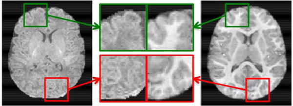
T1 MR image of a neonate (left) and its follow-up at two years of age (right). The 2-year-old image was aligned to the neonatal image by the nonlinear registration [45], [71]. Two brain regions marked with green and red blocks are zoomed in for closer comparison.

In the longitudinal studies of early brain development [72]–[74], all the high-quality MR images at different stages are needed to analyze brain growth trajectory and diagnose its health status for preventative care and treatment. For example, we know that autistic children have early brain overgrowth while the precise timing and magnitude of the overgrowth is not fully clear, and there are studies trying to address this question by measuring the size of brain structures at birth as well as other follow-up time points. However, small size and immature tissues of the neonatal brain result in poor spatial resolution, low SNR and severe blur of MR images in pediatric imaging. In this paper, we propose a novel longitudinally guided SR (LGSR) method for recovering an HR image from an LR neonatal image. The longitudinal follow-up images afford higher resolution and tissue contrast (see Fig. 1) for guiding resolution enhancement. The method proposed in this paper can help enhance the neonatal image quality for more accurate brain structure measurements. Although we have a more recent HR image of the subject, we still need to process the earlier image since the brain changes over time. Longitudinal analysis is useful for understanding normal and abnormal brain developmental process. The main contribution of this paper is twofold: 1) structural information from the longitudinal image is incorporated as a prior using guided bilateral filtering regularization (GBFR) and 2) GBF, low-rank, and TV regularizations are incorporated into an image SR framework for accurate estimation of the HR neonatal image. Our LGSR was evaluated in comparison with the state-of-the-art methods both qualitatively and quantitatively on a set of neonatal images.

In our previous work, we proposed an LRTV method [31] for MR image SR and then generalized it to LGSR by introducing a longitudinal prior as a nonlocal guided penalty in our published conference paper [46]. The nonlocal guided penalty is constructed based on the difference between the desired HR neonatal image and its nonlocal means (NLM) [16] jointly weighted by the high-quality longitudinal image. This paper serves two purposes. One is to provide additional method details, examples, results, discussion, and insights that are not presented in our conference publication [46]. The other is to introduce a modification for computation acceleration, which uses bilateral filtering (BF), instead of NLM filtering [16], because BF has lower computational cost. In experiments, we found the performance was similar for NLM [16] and BF used in this paper. The remainder of this paper is organized as follows. Section II describes LGSR in detail. Section III provides the experimental results and discussion. Section IV concludes this paper.

II. Method

In this section, we flesh out the LGSR method, which outputs an HR neonatal image from an LR neonatal image with its longitudinal follow-up image. We briefly review relevant works in Section II-A, describe the GBF-based longitudinal prior in Section II-B, and elaborate on the proposed SR model in Section II-C. We provide a numerical solution to the optimization problem in Section II-D.

A. Super-Resolution Model

In the SR problem, a physical model [1], [12] for describing the degradation process from an HR image to an LR image is generally given by

$$T=\mathit{DSX}+n$$ (1)

where T is the observed LR image, D is a downsampling operator, S is a blurring operator, X is the original HR image, and n denotes the noise. According to the observation model in (1), the goal of image SR is to recover an HR image from an observed LR image. Due to the ill-posed nature of the inverse problem, the regularization is introduced to eliminate the uncertainty of recovery. In the case of image SR, the HR image can be estimated by minimizing the objective cost function in the following form:

$$\widehat{X}=\underset{X}{min}{\Vert T-\mathit{DSX}\Vert }^2+\lambda \mathrm{\Phi }(X)$$ (2)

where ‖T − DSX‖² is the data fidelity term for penalizing the difference between the observed LR image T and the degraded version of HR image X, Φ(X) is a regularization term often defined on prior knowledge for stabilizing the solution, and the parameter λ is used to balance the tradeoff between the data fidelity term and the regularization term. The classical regularization methods reported in the literature includes the Tikhonov regularization [47], TV [48], [49], the nonlocal regularization [50], the sparsity regularization [9], [11], [12], and the nuclear norm regularization [31], [51], [52].

B. Guided Bilateral Filtering

Longitudinal images of an identical subject have very similar structural patterns. We borrow similar structural information from a longitudinal image to guide neonatal image SR. GBF is used to capture structural relationship. First, the spline interpolation is used to initialize the HR image X from an input LR neonatal image T. Then for each voxel ν in X, the similarity between the voxel ν and its neighbor κ in a cubic neighborhood Ω(ν) centered at ν is calculated based on the Euclidean distance ‖ν − κ‖ and the intensity difference ‖x(ν) − x(κ)‖ of the voxel ν and its neighbor κ in the HR image X. Using Gaussian functions, these distances are used to construct a weight map w_x to encode the relationship between voxel ν and voxel κ. Like w_x, the longitudinal weight map w_l for voxel ν with respect to the longitudinal follow-up image L is also generated based on the Euclidean distance ‖ν − κ‖ and the intensity difference ‖l(ν) − l(κ)‖. Weight maps w_x and w_l are combined to form a weight map w through element-wise multiplication. From X, GBF estimates the filtered HR neonatal image Y via weighted averaging

$$\begin{gathered} y(v)=\frac{1}{W_p}{\displaystyle {\sum }_{\kappa \in \mathrm{\Omega }(v)}x(\kappa )w(v,\kappa )} \\ =\frac{1}{W_p}{\displaystyle {\sum }_{\kappa \in \mathrm{\Omega }(v)}x(\kappa )w(v,\kappa )w_l(v,\kappa )} \end{gathered}$$ (3)

where y(ν) is the intensity of voxel ν in Y. The weights are defined as

$$w_x(v,\kappa )=\exp \left(-{\Vert x(v)-x(\kappa )\Vert }^2/2h_x^2-{\Vert v-\kappa \Vert }^2/2{\sigma }_x^2\right)$$ (4)

$$w_l(v,\kappa )=\exp \left(-{\Vert l(v)-l(\kappa )\Vert }^2/2h_l^2-{\Vert v-\kappa \Vert }^2/2{\sigma }_l^2\right)$$ (5)

where exp(·) is the Gaussian function, and σ_l, σ_x, h_l, and h_x are the parameters that control the decay rates of the Gaussian functions. The normalizing factor

$$W_p={\displaystyle {\sum }_{\kappa \in \mathrm{\Omega }(v)}{w}_x(v,\kappa )w_l(v,\kappa )}$$ (6)

makes sure that the weights sum to unity.

Combining the weights determined by the neonatal image and its longitudinal image increases robustness to structural misalignments. To illustrate this, we generate a degraded version of the neonatal image by Gaussian blurring with the blur kernel width of 1 and downsampling with the scaling factor of 2. Both the upsampled HR image X and the longitudinal image L as described above are used to estimate the weight map. The benefit of utilizing longitudinal information is illustrated in Fig. 2. Based on X, the neighboring weight map for a voxel near the anterior horn is shown in Fig. 2(a). This weight map does not truly reflect the local pattern of the anterior horn. The longitudinal image provides additional information as shown in Fig. 2(b). The two weight maps are merged into one weight map, shown in Fig. 2(c), which closely resembles the result given by the original HR neonatal image, shown in Fig. 2(d).

Fig. 2.

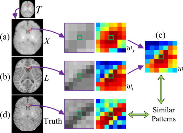
Advantages of the combined weight map. (a) Degraded neonatal image T and the upsampled HR image X, (b) longitudinal image L, (c) combined weight w from (a) w_x and (b) w_l, and (d) original HR neonatal image. The reference voxel is marked by green.

C. Longitudinally Guided Super-Resolution

The LGSR algorithm uses information from longitudinal data for neonatal image SR. The associated problem involves three regularization terms

$$\begin{gathered} \widehat{X}=\underset{X}{min}{\Vert T-\mathit{DSX}\Vert }^2+{\lambda }_{\text{GBF}}{\Vert X-Y\Vert }^2 \\ +{\lambda }_{\text{LR}}\text{Rank}(X)+{\lambda }_{\text{TV}}{\displaystyle \int |\nabla X|\mathit{dxdydz}} \end{gathered}$$ (7)

where λ_GBF, λ_LR, and λ_TV are the regularization parameters, Y as defined in (3) is the filtered HR neonatal image obtained from the desired HR neonatal image X and its longitudinal image L, Rank(·) denotes the rank of 3-D image matrix, |·| denotes the ℓ₂ norm, and ∇ is the gradient operator. Starting from the second term on the right side of (7) are GBF, low-rank, and TV regularization terms. These regularization terms are described below.

1) GBFR

Bilateral filter is a simple nonlinear filtering approach to smooth images while preserving strong edges by weighting the neighboring pixels based on their intensity similarity and spatial distance [53]. It has been widely used in image processing applications, such as image denoising [54] and fusion [55]. Petschnigg et al. [56] presented a joint bilateral filter to synthesize a high-quality image from a pair of flash and no-flash images. Inspired by their work, we extend the bilateral filter to include longitudinal information to regularize the SR problem. GBFR exploits structural redundancy between a neonatal image and its longitudinal image for reducing estimation uncertainty.

2) Low-Rank Regularization

Low-rank assumption is often used in matrix completion problems [52], where the task is to fill missing entries of an incomplete matrix. We use low-rank regularization to correct the corrupted structures by exploiting the inherent redundancy in the neonatal image. The rank of 3-D image matrix is defined as [57]: $\text{Rank}(X)={\displaystyle {\sum }_{i=1}^3{\alpha }_i}{\Vert X_{(i)}\Vert }_{\text{tr}}$, where the rank is computed as the sum of trace norms of all matrices unfolded along each dimension. ‖·‖ denotes the trace norm of a 2-D matrix. The parameters {α_i|i = 1, 2, 3} satisfy the condition that α_i ≫ 0 and ${\displaystyle {\sum }_{i=1}^3{\alpha }_i=1}$. The 2-D matrix X_(i) is the unfolded version of the 3-D image X along the ith dimension.

3) TV Regularization

The TV of a differentiable function can be defined as an integral of the absolute gradients [48]. The TV regularization [48], [49] has shown powerful ability to simultaneously preserve edges whilst smoothing noise in flat regions.

D. Optimization Solution

We employ the alternating direction method of multipliers (ADMM) algorithm [58] to solve the minimization problem (7). In order to facilitate solving this optimization problem, we introduce an auxiliary variable ${\left\{M_i\right\}}_{i=1}^3$ and an equality constraint X_(i) = M_i(i). Equation (7) can be reformulated as the augmented Lagrangian function [58]

$$\begin{gathered} \underset{X,{\left\{M_i\right\}}_{i=1}^3,{\left\{U_i\right\}}_{i=1}^3}{min}{\Vert T-\mathit{DSX}\Vert }^2+{\lambda }_{\text{GBF}}{\Vert X-Y\Vert }^2 \\ +{\displaystyle {\sum }_{i=1}^3\frac{\rho }{2}\left({\Vert X-M_i+A_i\Vert }^2-{\Vert A_i\Vert }^2\right)} \\ +{\lambda }_{\text{LR}}{\displaystyle {\sum }_{i=1}^3{\alpha }_i{\Vert M_{i(i)}\Vert }_{\text{tr}}+{\lambda }_{\text{TV}}}{\displaystyle \int |\nabla X_i|\mathit{dxdydz}} \end{gathered}$$ (8)

where the parameter ρ > 0, and ${\left\{A_i\right\}}_{i=1}^3$ is the Lagrangian dual variable to integrate the equality constraint into the cost function. Note that we can keep the guided bilateral filtered image Y fixed so that the optimization problem (8) is convex. By using the scaled dual variable, we can express ADMM for the cost function in (8) as three subproblems.

1) Subproblem 1

Keep ${\left\{M_i\right\}}_{i=1}^3$ and ${\left\{A_i\right\}}_{i=1}^3$ fixed, and update X^(k+1) by minimizing the subproblem

$$\begin{gathered} X^{(k+1)}=\underset{X}{min}{\Vert T-\mathit{DSX}\Vert }^2+{\lambda }_{\text{GBF}}{\Vert X-Y\Vert }^2 \\ +{\displaystyle {\sum }_{i=1}^3\frac{\rho }{2}\left({\Vert X-M_i^{(k)}+A_i^{(k)}\Vert }^2\right)} \\ +{\lambda }_{\text{TV}}{\displaystyle \int |\nabla X|\mathit{dxdydz}.} \end{gathered}$$ (9)

This subproblem can be solved by the gradient descent method, where the spatial gradient of the image X for the TV regularization can be obtained by the related Euler–Lagrange equation in the iterative solution [59].

2) Subproblem 2

Keep X and ${\left\{A_i\right\}}_{i=1}^3$ fixed, and update

$$\begin{gathered} {\left\{M_i^{(k+1)}\right\}}_{i=1}^3=\underset{{\left\{M_i\right\}}_{i=1}^3}{min}{\lambda }_{\text{LR}}{\displaystyle {\sum }_{i=1}^3{\alpha }_i{\Vert M_{i(i)}\Vert }_{\text{tr}}} \\ +{\displaystyle {\sum }_{i=1}^3\frac{\rho }{2}\left({\Vert X^{(k+1)}-M_i+A_i^{(k)}\Vert }^2\right)}. \end{gathered}$$ (10)

According to the singular value thresholding (SVT) [52], an iterative converged solution to (10) is given by

$$\{\begin{array}{l}(U,\sum ,V)=\text{svd}\left(X_{(i)}^{(k+1)}+A_{i(i)}^{(k)}\right)\hfill \\ {\widehat{\sum }}_{jj}=max({\sum }_{jj}-2{\lambda }_{\text{LR}}{\alpha }_i/\rho ,0)\hfill \\ M_{i(i)}^{(k+1)}=U\widehat{\sum }{V}^T\hfill \end{array}$$ (11)

where svd denotes the singular value decomposition operator, and Σ_jj is the singular value at location (j, j) that is shrinked as ${\widehat{\sum }}_{jj}$ at the iteration k.

3) Subproblem 3

Keep X and ${\left\{M_i\right\}}_{i=1}^3$ fixed, and update ${\left\{A_i^{(k+1)}\right\}}_{i=1}^3$ by minimizing the subproblem

$$A_i^{(k+1)}=A_i^{(k)}+\left(X^{(k+1)}-M_i^{(k+1)}\right).$$ (12)

These three subproblems are separately solved and updated until convergence. The convergence condition is that an iterative difference of the cost function in (8) is less than the allowable error ε. LGSR is summarized in Algorithm 1.

III. Experiments

A. Test Data

MR images of 28 healthy infants were obtained from a large study of early brain development in normal children [60].

Algorithm 1.

Pseudocode of the LGSR Algorithm.

Input: LR neonatal image T and HR longitudinal image L.

Output: Reconstructed HR neonatal image X.

Initialize the desired HR neonatal image X by upsampling T with spline-based interpolation. Set auxiliary variables Mi = 0, Ai = 0, i = 1, 2, 3.

Repeat

Update Y based on Eqs. (3) to (6);

Repeat

Update X via Eq. (9) by the gradient descent method;

Update M based on Eqs. (10) and (11) by SVT [52];

Update A based on Eq. (12);

End

Until convergence;

End

The experimental protocols were approved by the institutional review board of the University of North Carolina, School of Medicine. These infants consist of 11 males and 17 females. They were first scanned at birth, and then a follow-up scan was performed at two years of age, by the 3T MRI head-only scanner (Siemens MAGNETOM Tim Trio) with a circular polarized 32-channel head coil. The two most common types of MR images (i.e., T1 and T2 images) were generated as test data. T1 images were acquired by using short echo time (TE) and repetition time (TR). Conversely, T2 images were produced by using long TE and TR times. For a subject, T1 images were acquired with 144 sagittal slices at the resolution of 1 × 1 × 1 mm³, while T2 images were obtained with 58 axial slices at the resolution of 1.25 × 1.25 × 1.95 mm³. These images were preprocessed by a standard image processing pipeline including bias correction and skull stripping [61]. The longitudinal follow-up images were aligned to their neonatal images with the affine registration [45] followed by the nonlinear diffeomorphic demons registration [62]. T2 images were also linearly aligned to their corresponding T1 images.

B. Experimental Setting

We simulated a set of LR neonatal images by applying Gaussian blurring with a blur kernel of 1 voxel wide and downsampling to the original neonatal images (Fig. 3), similar to LRTV [31]. For downsampling with a factor 2, every 8 voxels in a 3-D HR image were averaged to generate a corresponding voxel in the simulated LR image. The reconstructed HR images were compared with the original neonatal images regarded as the ground truth. For quantitative assessment, both full-reference and no-reference image quality assessment (IQA) metrics were employed to evaluate the SR performance of LGSR quantitatively. The similarity between the reconstructed image and the original image was measured by SNR, defined as SNR = 20 log(‖I_O‖/‖I_O − I_E‖), where I_O and I_E are the ground truth and the reconstructed image, respectively. In our experiments, the basic parameters of the proposed algorithm were set as follows: λ_GBF = 0.02, λ_LR = 0.01, α₁ = α₂ = α₃ = 1/3, ρ = 0.04, λ_TV = 0.01, dt = 0.1, σ_l = σ_x = 20, h_l = 0.01R_L, and h_x = 0.01R_X. Here, R_L and R_X denoted the intensity ranges of images L and X, respectively. The 3-D neighboring domain was 7 × 7 × 7 voxels. The program stopped when the difference between iterations was less than the allowable error ε = 10⁻⁵ or the maximum iteration number 200 was reached. To verify the robustness of LGSR, we treated the SNR values of reconstructed HR images as a function of a parameter change while keeping all other parameters at their default values. Fig. 4 shows SNR values given by LGSR against the changes of the regularization parameters λ_GBF, λ_LR, and λ_TV. Our LGSR method is sensitive to small variations of λ_GBF, but robust to relatively large changes of the other parameters (less than 0.1 dB difference in SNR) around the default values.

Fig. 3.

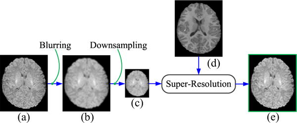
Simulation of an LR image from an original neonatal image. (a) Original neonatal image, (b) blurred image, (c) generated LR image, (d) aligned longitudinal image, and (e) recovered HR image.

Fig. 4.

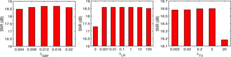
SNR values given by our LGSR in relation to various key parameters for a randomly selected neonate.

C. Results on Simulated Images

T1 and T2 imaging modalities were used in the following experiments. For these two modalities, the HR neonatal images with an upsampling factor of 2 were reconstructed from the input LR neonatal images with their corresponding longitudinal images. The proposed method was compared using the test data with the competing methods, including nearest neighbor (NN) interpolation, spline interpolation (spline) [5], NLMU [24], and LRTV [31], [63]. We adopted the code for NLMU [24]¹ and LRTV [31]² provided on the authors’ websites. The spline interpolation was used for the initialization of NLMU [24], LRTV [31], [63], and LGSR.

To evaluate the impact of the proposed GBFR on the SR performance, we chose a set of neonatal and longitudinal images from 28 subjects to test our method by setting one regularization parameter λ_GBF to the default value and the other parameters ρ, λ_LR, and λ_TV to zero. Given that there were two modalities and two time points, there were four possible combination of images to be used for SR: neonatal T1/longitudinal T1 (T1/T1), neonatal T1/longitudinal T2 (T1/T2), neonatal T2/longitudinal T1 (T2/T1), and neonatal T2/longitudinal T2 (T2/T2). For these test images, as one part of LGSR, GBFR was compared between LGSR and LRTV [31] to verify its superiority for SR improvement of LGSR. Fig. 5 gives compared SNR results of LRTV [31], the proposed GBFR and LGSR for four pairs of input test images from 28 subjects. For a random selection of four pairs of test data, the visual comparison of the axial results produced by LRTV [31], our GBFR and LGSR are shown in Fig. 6. As can be seen from Figs. 5 to 6, LGSR achieved great gain for image SR by incorporating the proposed GBFR. This improvement verified that the GBFR was beneficial and necessary to LGSR.

Fig. 5.

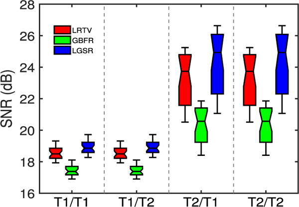
Impact of GBFR.

Fig. 6.

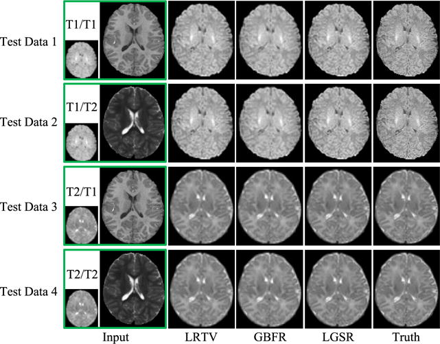
SR results obtained by LRTV [31], GBFR, and LGSR for four pairs of images.

For further qualitative assessment, we show the results of two randomly selected subjects in Fig. 7 (intramodality) and Fig. 8 (intermodality). From the figures, the results of NN and spline show severe blurring artifacts. The results of NLMU [24] also appear blurry to a certain extent due to the lack of explicit modeling of image degradation. LGSR is effective for neonatal image SR and achieves higher SNR than LRTV [31] and other compared methods. It can also be observed that the choice of longitudinal T1 or T2 image has little impact on the performance of the proposed algorithm. Therefore, we chose to use longitudinal images of the same modality in subsequent experiments.

Fig. 7.

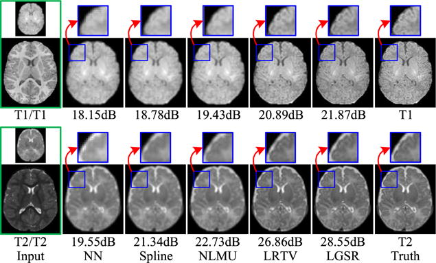
Intramodality SR results of LGSR in comparison with the competing methods for two neonatal subjects.

Fig. 8.

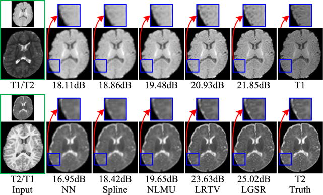
Intermodality SR results of LGSR in comparison with the competing methods for two neonatal subjects.

Quantitative evaluation was performed with three metrics: 1) SNR; 2) SSIM [64]; and 3) IFC [65] reported to be more consistent with perceptual scores [66]. Figs. 9 and 10 show, respectively, the box plots of SNR, SSIM, and IFC results of 28 reconstructed neonatal T1 and T2 images. The central line of each box is the median, the edges mark the 25th and 75th percentiles, and the whiskers extend to the minimum and the maximum. LGSR achieves the highest SNR, SSIM, and IFC among all methods for both T1 and T2 images. As a statistical inference tool, the two-sample t-test [67] was also used to assess whether or not LGSR exceeds the competing methods in SNR, SSIM, and IFC. The null hypothesis for this testing is that the mean values of SNR, SSIM and IFC obtained by LGSR are equal to those obtained by a competing method. The alternative hypothesis is that the mean values of SNR, SSIM, and IFC obtained by LGSR are larger than those obtained by a competing method. For the two groups of SNR, SSIM, or IFC results separately obtained by LGSR and a competing method, a test statistic (t-value) following a t-distribution is calculated with the appropriate degrees of freedom. After the t-value and the degrees of freedom are determined, a p-value is found by using a table of values from the t-distribution. If this p-value is below the significance level α_t (typically α_t = 0.05), then the null hypothesis is rejected in favor of the alternative hypothesis. Otherwise, there is no statistically significant difference between the two groups of SNR, SSIM, or IFC results. In Table I, the asteroid marks the p-values that are less than the threshold α_t = 0.05 chosen for statistical significance. These values imply that the means of SNR, SSIM and IFC results obtained by LGSR are significantly larger than those obtained by the competing methods, judging based on two-sample t-tests.

Fig. 9.

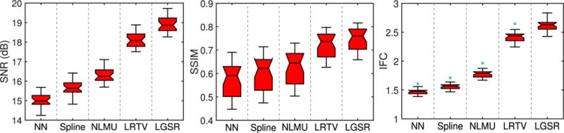
Box plots for SNR, SSIM, and IFC results of 28 reconstructed neonatal T1 images.

Fig. 10.

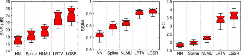
Box plots for SNR, SSIM, and IFC results of 28 reconstructed neonatal T2 images.

Table I.

p-Values of Two-Sample t-Tests of SNR (dB), SSIM, and IFC Results Between LGSR and the Competing Methods. Significant Improvements Are Marked by Asterisks Indicating That the p-Values Are Less Than the Threshold α_t (Typically α_t = 0.05) Chosen for Statistical Significance

Index		NN	Spline	NLMU	LRTV
T1/T1	SNR	0.0001*	0.0001*	0.0001*	0.0001*
	SSIM	0.0001*	0.0001*	0.0001*	0.0610
	IHC	0.00001*	0.00001*	0.00001*	0.00001*
T2/T2	SNR	0.0001*	0.0001*	0.0001*	0.0540
	SSIM	0.0001*	0.0001*	0.0001*	0.0270*
	IHC	0.00001*	0.00001*	0.00001*	0.0023*

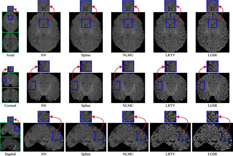
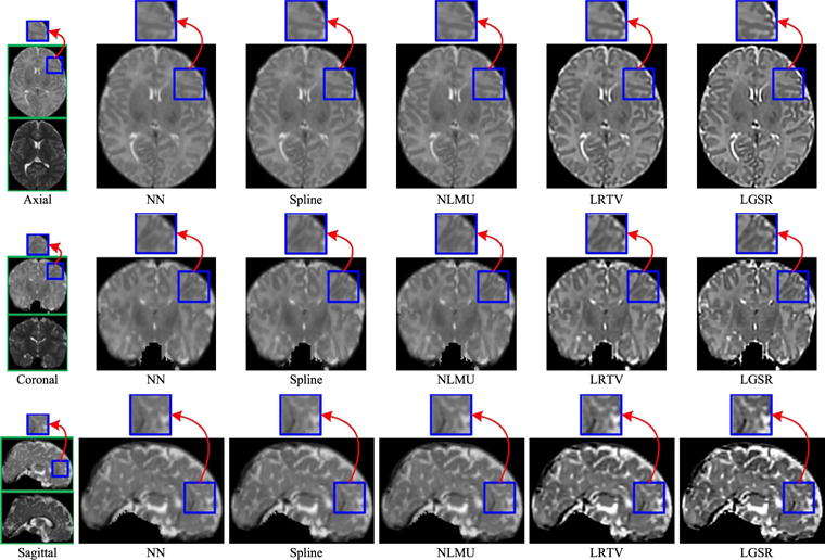
Fig. 11 shows the axial, sagittal, and coronal views of the reconstructed HR neonatal T1 images, indicating that LGSR recovers more anatomical details than the competing methods.

Fig. 11.

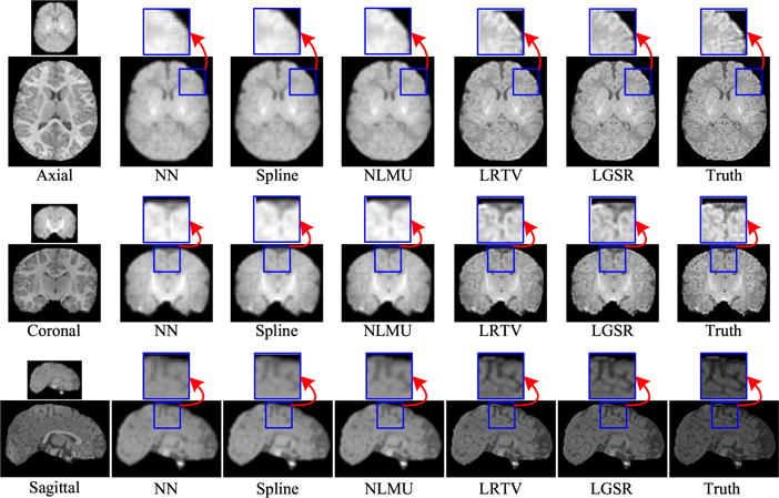
Visual comparison of axial, sagittal, and coronal views of reconstructed HR neonatal T1 images with close-up views of specific regions (the upscaling factor 2).

Considering that both the blur kernel width and scaling factor have a great impact on the SR performance, we also implemented another experiment to validate the proposed algorithm with different settings of blur kernel and scaling factors around their default values. For a randomly selected neonate, Fig. 12 provides SNR, SSIM, and IFC results obtained by NN, spline, NLMU [24], LRTV [31], and LGSR with different blur kernel widths σ_S and fixed scaling factor 2. Fig. 13 shows SNR, SSIM, and IFC results of these SR methods for the fixed blur kernel width (i.e., σ_S = 1) and different scaling factors. From the results, both the blur kernel width and scaling factor affect the SR performance greatly, but the proposed algorithm still generally outperforms the competing methods, and can achieve the best results by choosing the proper value of the blur kernel width for a given scaling factor.

Fig. 12.

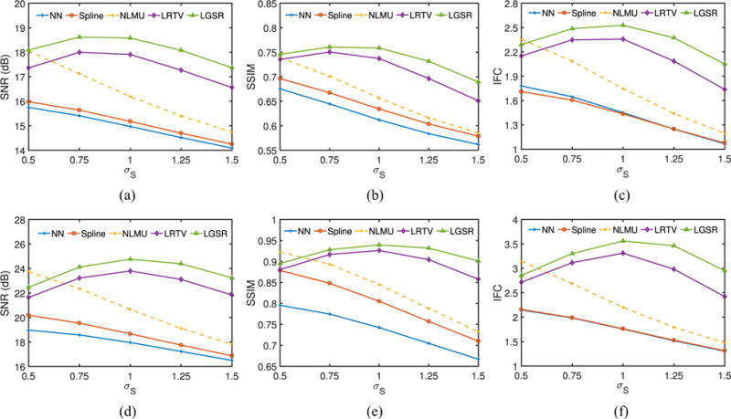
SNR, SSIM, and IFC results of a random neonate obtained by NN, spline, NLMU, LRTV, and LGSR with different blur kernel widths and the fixed scaling factor 2. (a) SNR for T1. (b) SSIM for T1. (c) IFC for T1. (d) SNR for T2. (e) SSIM for T2. (f) IFC for T2.

Fig. 13.

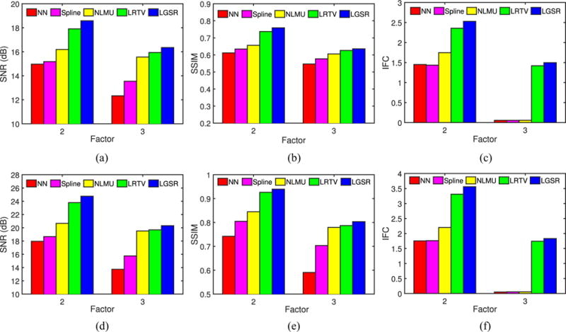
SNR, SSIM, and IFC results of a random neonate obtained by NN, spline, NLMU, LRTV, and LGSR with the fixed blur kernel width 1 and different scaling factors. (a) SNR for T1. (b) SSIM for T1. (c) IFC for T1. (d) SNR for T2. (e) SSIM for T2. (f) IFC for T2.

D. Tissue Segmentation

We performed further evaluation based on brain tissue segmentation of the 28 reconstructed HR neonatal images using a patch-driven level set method [68], where the brain tissues were separated into gray matter (GM), white matter (WM), and cerebrospinal fluid (CSF). These segmentation results were assessed by the Dice similarity coefficient (DSC) [69]. Fig. 14 gives example results generated based on reconstructed HR neonatal T2 images obtained by the various methods. Fig. 15 shows the box plots of DSC metrics for three brain tissues (GM/WM/CSF). The segmentation results of the original HR neonatal brain images were used as the benchmark. Figs. 14 and 15 show that the segmentation results of LGSR are closer to the benchmark than the competing methods.

Fig. 14.

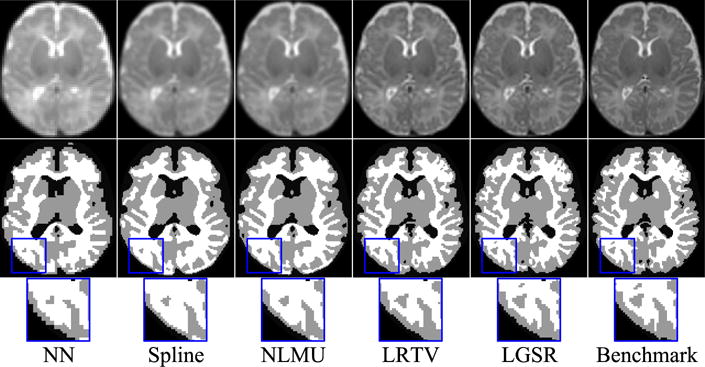
Tissue segmentation results by LGSR and the competing methods. From top to bottom: reconstructed HR neonatal T2 images, segmentation results, and close-up views.

Fig. 15.

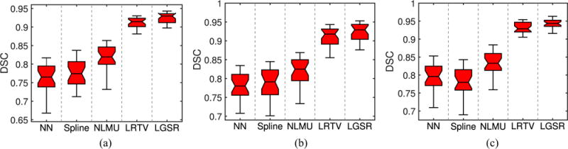
DSC values for tissue segmentation of reconstructed HR neonatal T2 brain images by LGSR and the competing methods. (a) GM. (b) WM. (c) CSF.

E. Results on Real Images

Besides the experiments on the simulated LR images mentioned above, we also performed another experiment on real neonatal images to validate the SR performance of the proposed LGSR method. Without loss of generality, in this paper, we gave the visual results of LGSR and the baseline methods [24], [31] by randomly selecting a real neonatal image and its longitudinal image of the same modality from an identical subject. Figs. 16 and 17 show the visual comparison of SR results by NN, spline, NLMU [24], LRTV [31] and our LGSR for T1 and T2 images, respectively. From Figs. 16 to 17, the SR results of our LGSR have clear anatomical structures with fine details, whereas those of NN, spline, NLMU [24] and LRTV [31] are blurred with smooth edges. This experiment on real images further verified that our LGSR is superior to the state-of-the-art methods for neonatal brain image SR.

Fig. 16.

Visual comparison of the results obtained by the different methods for a real neonatal T1 image with its longitudinal T1 image from an identical subject (the scaling factor 2).

Fig. 17.

Visual comparison of the results obtained by the different methods for a real neonatal T2 image with its longitudinal T2 image from an identical subject (the scaling factor 2).

F. Discussion

Besides the full-reference IQA on the SR results from simulated MR images using three metrics (i.e., SNR, SSIM [64], and IFC [65]) in the quantitative evaluation, we also adopted the perception-driven no-reference metric (PNM) [70] to assess the SR results from real MR images due to the lack of the ground-truth images in practice. Fig. 18 gives box plots of PNM results of reconstructed SR images with the upscaling factor 2 from 28 real LR neonatal T1/T2 images. From Fig. 18, PNM score of NN is better than that of spline, but both Figs. 16 and 17 show that NN is worse than spline in visual quality assessment. Even though PNM [70] achieves great success for no-reference IQA of natural images, the inconsistent evaluation from Figs. 16 to 18 implies that PNM [70] cannot be directly applied to quantitative quality assessment of real MR images due to their noise and blur.

Fig. 18.

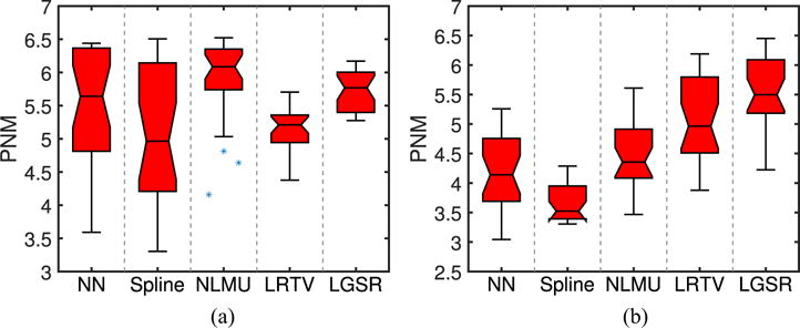
Box plots of PNM results of reconstructed SR images from 28 real LR neonatal T1/T2 images. (a) T1. (b) T2.

IV. Conclusion

In this paper, we addressed the neonatal image SR problem by incorporating a longitudinal image prior, in combination with the low-rank constraint and the TV regularization. The ADMM method is used to solve the associated optimization problem. The experimental results demonstrate that the proposed LGSR algorithm outperforms existing state-of-the-art methods both qualitatively and quantitatively. Besides, the images from more than two time points will be included for further improving performance and efficiency of neonatal image SR reconstruction.

References

- 1.Park SC, Park MK, Kang MG. Super-resolution image reconstruction: A technical overview. IEEE Signal Process Mag. 2003 May;20(3):21–36. [Google Scholar]
- 2.Freeman WT, Jones TR, Pasztor EC. Example-based super-resolution. IEEE Comput Graph Appl. 2002 Mar-Apr;22(2):56–65. [Google Scholar]
- 3.Pham DL, Xu C, Prince JL. Current methods in medical image segmentation. Annu Rev Biomed Eng. 2000;2(1):315–337. doi: 10.1146/annurev.bioeng.2.1.315. [DOI] [PubMed] [Google Scholar]
- 4.Farsiu S, Robinson D, Elad M, Milanfar P. Advances and challenges in super-resolution. Int J Imag Syst Technol. 2004;14(2):47–57. [Google Scholar]
- 5.Lehmann T, Gonner C, Spitzer K. Survey: Interpolation methods in medical image processing. IEEE Trans Med Imag. 1999 Nov;18(11):1049–1075. doi: 10.1109/42.816070. [DOI] [PubMed] [Google Scholar]
- 6.Li X, Orchard MT. New edge-directed interpolation. IEEE Trans Image Process. 2001 Oct;10(10):1521–1527. doi: 10.1109/83.951537. [DOI] [PubMed] [Google Scholar]
- 7.Huang J-J, Siu W-C, Liu T-R. Fast image interpolation via random forests. IEEE Trans Image Process. 2015 Oct;24(10):3232–3245. doi: 10.1109/TIP.2015.2440751. [DOI] [PubMed] [Google Scholar]
- 8.Protter M, Elad M, Takeda H, Milanfar P. Generalizing the nonlocal-means to super-resolution reconstruction. IEEE Trans Image Process. 2009 Jan;18(1):36–51. doi: 10.1109/TIP.2008.2008067. [DOI] [PubMed] [Google Scholar]
- 9.Daubechies I, Defrise M, De Mol C. An iterative thresholding algorithm for linear inverse problems with a sparsity constraint. Commun Pure Appl Math. 2004;57(11):1413–1457. [Google Scholar]
- 10.Zhang K, Gao X, Tao D, Li X. Single image super-resolution with non-local means and steering kernel regression. IEEE Trans Image Process. 2012 Nov;21(11):4544–4556. doi: 10.1109/TIP.2012.2208977. [DOI] [PubMed] [Google Scholar]
- 11.Candes E, Wakin M, Boyd S. Enhancing sparsity by reweighted l(1) minimization. J Fourier Anal Appl. 2008;14(5–6):877–905. [Google Scholar]
- 12.Zhang Y, Liu J, Yang W, Guo Z. Image super-resolution based on structure-modulated sparse representation. IEEE Trans Image Process. 2015 Sep;24(9):2797–2810. doi: 10.1109/TIP.2015.2431435. [DOI] [PubMed] [Google Scholar]
- 13.Shen H, Peng L, Yue L, Yuan Q, Zhang L. Adaptive norm selection for regularized image restoration and super-resolution. IEEE Trans Cybern. 2016 Jun;46(6):1388–1399. doi: 10.1109/TCYB.2015.2446755. [DOI] [PubMed] [Google Scholar]
- 14.Fattal R. Image upsampling via imposed edge statistics. ACM Trans Graph. 2007;26(3):95. [Google Scholar]
- 15.Yan Q, Xu Y, Yang X, Nguyen TQ. Single image superresolution based on gradient profile sharpness. IEEE Trans Image Process. 2015 Oct;24(10):3187–3202. doi: 10.1109/TIP.2015.2414877. [DOI] [PubMed] [Google Scholar]
- 16.Buades A, Coll B, Morel JM. A review of image denoising algorithms, with a new one. Multiscale Model Simulat. 2005;4(2):490–530. [Google Scholar]
- 17.Zhang Y, Liu J, Li M, Guo Z. Joint image denoising using adaptive principal component analysis and self-similarity. Inf Sci. 2014 Feb;259:128–141. [Google Scholar]
- 18.Jiang J, et al. Single image super-resolution via locally regularized anchored neighborhood regression and nonlocal means. IEEE Trans Multimedia. 2017 Jan;19(1):15–26. [Google Scholar]
- 19.Yu GS, Sapiro G, Mallat S. Solving inverse problems with piecewise linear estimators: From Gaussian mixture models to structured sparsity. IEEE Trans Image Process. 2012 May;21(5):2481–2499. doi: 10.1109/TIP.2011.2176743. [DOI] [PubMed] [Google Scholar]
- 20.Zhang Y, Xiao J, Li S, Shi C, Xie G. Learning block-structured incoherent dictionaries for sparse representation. Sci China Inf Sci. 2015;58(10):1–15. [Google Scholar]
- 21.Jiang J, Ma X, Cai Z, Hu R. Sparse support regression for image super-resolution. IEEE Photon J. 2015 Oct;7(5):1–11. [Google Scholar]
- 22.Jiang J, Ma J, Chen C, Jiang X, Wang Z. Noise robust face image super-resolution through smooth sparse representation. IEEE Trans Cybern. 2017 Nov;47(11):3991–4002. doi: 10.1109/TCYB.2016.2594184. [DOI] [PubMed] [Google Scholar]
- 23.Van Reeth E, Tham IWK, Tan CH, Poh CL. Super-resolution in magnetic resonance imaging: A review. Concepts Magn Reson A. 2012;40(6):306–325. [Google Scholar]
- 24.Manjón JV, et al. Non-local MRI upsampling. Med Image Anal. 2010;14(6):784–792. doi: 10.1016/j.media.2010.05.010. [DOI] [PubMed] [Google Scholar]
- 25.Rousseau F. A non-local approach for image super-resolution using intermodality priors. Med Image Anal. 2010;14(4):594–605. doi: 10.1016/j.media.2010.04.005. [DOI] [PMC free article] [PubMed] [Google Scholar]
- 26.Rueda A, Malpica N, Romero E. Single-image super-resolution of brain MR images using overcomplete dictionaries. Med Image Anal. 2013;17(1):113–132. doi: 10.1016/j.media.2012.09.003. [DOI] [PubMed] [Google Scholar]
- 27.Trinh D-H, et al. Novel example-based method for super-resolution and denoising of medical images. IEEE Trans Image Process. 2014 Apr;23(4):1882–1895. doi: 10.1109/TIP.2014.2308422. [DOI] [PubMed] [Google Scholar]
- 28.Tourbier S, et al. An efficient total variation algorithm for super-resolution in fetal brain MRI with adaptive regularization. NeuroImage. 2015 Sep;118:584–597. doi: 10.1016/j.neuroimage.2015.06.018. [DOI] [PubMed] [Google Scholar]
- 29.Ben-Ari R, Sochen N. Stereo matching with Mumford–Shah regularization and occlusion handling. IEEE Trans Pattern Anal Mach Intell. 2010 Nov;32(11):2071–2084. doi: 10.1109/TPAMI.2010.32. [DOI] [PubMed] [Google Scholar]
- 30.Xiao J, et al. Multi-focus image fusion based on depth extraction with inhomogeneous diffusion equation. Signal Process. 2016 Aug;125:171–186. [Google Scholar]
- 31.Shi F, Cheng J, Wang L, Yap P-T, Shen D. LRTV: MR image super-resolution with low-rank and total variation regularizations. IEEE Trans Med Imag. 2015 Dec;34(12):2459–2466. doi: 10.1109/TMI.2015.2437894. [DOI] [PMC free article] [PubMed] [Google Scholar]
- 32.Dong C, Loy CC, He K, Tang X. Learning a deep convolutional network for image super-resolution. in Proc Eur Conf Comput Vis. 2014:184–199. [Google Scholar]
- 33.Dong C, Loy CC, He K, Tang X. Image super-resolution using deep convolutional networks. IEEE Trans Pattern Anal Mach Intell. 2016 Feb;38(2):295–307. doi: 10.1109/TPAMI.2015.2439281. [DOI] [PubMed] [Google Scholar]
- 34.Dong C, Loy C, Tang X. Accelerating the super-resolution convolutional neural network. in Proc Eur Conf Comput Vis. 2016:391–407. [Google Scholar]
- 35.Ledig C, et al. Photo-realistic single image super-resolution using a generative adversarial network. in Proc IEEE Comput Vis Pattern Recognit. 2017:105–114. [Google Scholar]
- 36.Kim J, Lee JK, Lee KM. Deeply-recursive convolutional network for image super-resolution. in Proc IEEE Comput Vis Pattern Recognit. 2016:1637–1645. [Google Scholar]
- 37.Tai Y, Yang J, Liu X. Image super-resolution via deep recursive residual network. in Proc IEEE Comput Vis Pattern Recognit. 2017:2790–2798. [Google Scholar]
- 38.Wang Z, Liu D, Yang J, Han W, Huang T. Deep networks for image super-resolution with sparse prior. in Proc IEEE Int Conf Comput Vis. 2015:370–378. [Google Scholar]
- 39.Mao X, Shen C, Yang Y. Image restoration using very deep convolutional encoder-decoder networks with symmetric skip connections. in Proc Adv Neural Inf Process Syst. 2016:2802–2810. [Google Scholar]
- 40.Johnson J, Alahi A, Li F. Perceptual losses for real-time style transfer and super-resolution. in Proc Eur Conf Comput Vis. 2016:694–711. [Google Scholar]
- 41.Lai W-S, Huang J-B, Ahuja N, Yang M-H. Deep Laplacian pyramid networks for fast and accurate super-resolution. in Proc IEEE Comput Vis Pattern Recognit. 2017:5835–5843. [Google Scholar]
- 42.Shi F, et al. Neonatal brain image segmentation in longitudinal MRI studies. NeuroImage. 2010;49(1):391–400. doi: 10.1016/j.neuroimage.2009.07.066. [DOI] [PMC free article] [PubMed] [Google Scholar]
- 43.Wang L, et al. Longitudinally guided level sets for consistent tissue segmentation of neonates. Human Brain Mapping. 2013;34(4):956–972. doi: 10.1002/hbm.21486. [DOI] [PMC free article] [PubMed] [Google Scholar]
- 44.Armstrong E, Schleicher A, Omran H, Curtis M, Zilles K. The ontogeny of human gyrification. Cerebral Cortex. 1995;5(1):56–63. doi: 10.1093/cercor/5.1.56. [DOI] [PubMed] [Google Scholar]
- 45.Fischer J, del Rio A. A fast method for applying rigid transformations to volume data. in Proc Int Conf Central Europe Comput Graph Vis Comput Vis. 2004:55–62. [Google Scholar]
- 46.Shi F, Cheng J, Wang L, Yap P-T, Shen D. Longitudinal guided super-resolution reconstruction of neonatal brain MR images. in Proc Int Workshop Spatio Temporal Image Anal Longitudinal Time Series Image Data. 2014:67–76. doi: 10.1007/978-3-319-14905-9_6. [DOI] [PMC free article] [PubMed] [Google Scholar]
- 47.Golub GH, Hansen PC, O’Leary DP. Tikhonov regularization and total least squares. SIAM J Matrix Anal Appl. 1999;21(1):185–194. [Google Scholar]
- 48.Rudin LI, Osher S, Fatemi E. Nonlinear total variation based noise removal algorithms. Physica D Nonlin Phenomena. 1992;60(1–4):259–268. [Google Scholar]
- 49.Osher S, Burger M, Goldfarb D, Xu J, Yin W. An iterative regularization method for total variation-based image restoration. Multiscale Model Simulat. 2005;4(2):460–489. [Google Scholar]
- 50.Peyré G, Bougleux S, Cohen L. Non-local regularization of inverse problems. Inverse Problems Imag. 2011;5(2):511–530. [Google Scholar]
- 51.Recht B, Fazel M, Parrilo PA. Guaranteed minimum-rank solutions of linear matrix equations via nuclear norm minimization. SIAM Rev. 2010;52(3):471–501. [Google Scholar]
- 52.Cai J-F, Candes EJ, Shen Z. A singular value thresholding algorithm for matrix completion. SIAM J Optim. 2010;20(4):1956–1982. [Google Scholar]
- 53.Tomasi C, Manduchi R. Bilateral filtering for gray and color images. Proc Int Conf Comput Vis. 1998:839–846. [Google Scholar]
- 54.Zhang B, Allebach J. Adaptive bilateral filter for sharpness enhancement and noise removal. IEEE Trans Image Process. 2008 May;17(5):664–678. doi: 10.1109/TIP.2008.919949. [DOI] [PubMed] [Google Scholar]
- 55.Zhou Z, Wang B, Li S, Dong M. Perceptual fusion of infrared and visible images through a hybrid multi-scale decomposition with Gaussian and bilateral filters. Inf Fusion. 2016 Jun;30:15–26. [Google Scholar]
- 56.Petschnigg G, et al. Digital photography with flash and no-flash image pairs. ACM Trans Graph. 2004;23(3):664–672. [Google Scholar]
- 57.Liu J, Musialski P, Wonka P, Ye J. Tensor completion for estimating missing values in visual data. IEEE Trans Pattern Anal Mach Intell. 2013 Jan;35(1):208–220. doi: 10.1109/TPAMI.2012.39. [DOI] [PubMed] [Google Scholar]
- 58.Boyd S, Parikh N, Chu E, Peleato B, Eckstein J. Distributed optimization and statistical learning via the alternating direction method of multipliers. Found Trends Mach Learn. 2011;3(1):1–122. [Google Scholar]
- 59.Marquina A, Osher SJ. Image super-resolution by TV-regularization and Bregman iteration. J Sci Comput. 2008;37(3):367–382. [Google Scholar]
- 60.Gilmore JH, et al. Regional gray matter growth, sexual dimorphism, and cerebral asymmetry in the neonatal brain. J Neurosci. 2007;27(6):1255–1260. doi: 10.1523/JNEUROSCI.3339-06.2007. [DOI] [PMC free article] [PubMed] [Google Scholar]
- 61.Shi F, et al. LABEL: Pediatric brain extraction using learning-based meta-algorithm. NeuroImage. 2012;62(3):1975–1986. doi: 10.1016/j.neuroimage.2012.05.042. [DOI] [PMC free article] [PubMed] [Google Scholar]
- 62.Vercauteren T, Pennec X, Perchant A, Ayache N. Diffeomorphic demons: Efficient non-parametric image registration. NeuroImage. 2009;45(1):S61–S72. doi: 10.1016/j.neuroimage.2008.10.040. [DOI] [PubMed] [Google Scholar]
- 63.Shi F, Cheng J, Wang L, Yap P-T, Shen D. Low-rank total variation for image super-resolution. in Proc Int Conf Med Image Comput Comput Assist Intervent. 2013:155–162. doi: 10.1007/978-3-642-40811-3_20. [DOI] [PMC free article] [PubMed] [Google Scholar]
- 64.Wang Z, Bovik AC, Sheikh HR, Simoncelli EP. Image quality assessment: From error visibility to structural similarity. IEEE Trans Image Process. 2004 Apr;13(4):600–612. doi: 10.1109/tip.2003.819861. [DOI] [PubMed] [Google Scholar]
- 65.Sheikh HR, Bovik AC, de Veciana G. An information fidelity criterion for image quality assessment using natural scene statistics. IEEE Trans Image Process. 2005 Dec;14(12):2117–2128. doi: 10.1109/tip.2005.859389. [DOI] [PubMed] [Google Scholar]
- 66.Yang C-Y, Ma C, Yang M-H. Single-image super-resolution: A benchmark. in Proc Eur Conf Comput Vis. 2014:372–386. [Google Scholar]
- 67.Krzywinski M, Altman N. Points of significance: Significance, P values and t-tests. Nat Methods. 2013;10(11):1041–1042. doi: 10.1038/nmeth.2698. [DOI] [PubMed] [Google Scholar]
- 68.Wang L, et al. Segmentation of neonatal brain MR images using patch-driven level sets. NeuroImage. 2014 Jan;84:141–158. doi: 10.1016/j.neuroimage.2013.08.008. [DOI] [PMC free article] [PubMed] [Google Scholar]
- 69.Taha AA, Hanbury A. Metrics for evaluating 3D medical image segmentation: Analysis, selection, and tool. BMC Med Imag. 2015;15(1):29. doi: 10.1186/s12880-015-0068-x. [DOI] [PMC free article] [PubMed] [Google Scholar]
- 70.Ma C, Yang C-Y, Yang X, Yang M-H. Learning a no-reference quality metric for single-image super-resolution. Comput Vis Image Understanding. 2017 May;158:1–16. [Google Scholar]
- 71.Xue Z, Shen D, Davatzikos C. Statistical representation of high-dimensional deformation fields with application to statistically constrained 3D warping. Med Image Anal. 2006;10(5):740–751. doi: 10.1016/j.media.2006.06.007. [DOI] [PubMed] [Google Scholar]
- 72.Shi F, et al. Construction of multi-region-multi-reference atlases for neonatal brain MRI segmentation. Neuroimage. 2010;51(2):684–693. doi: 10.1016/j.neuroimage.2010.02.025. [DOI] [PMC free article] [PubMed] [Google Scholar]
- 73.Lyall AE, et al. Dynamic development of regional cortical thickness and surface area in early childhood. Cerebral Cortex. 2014;25(8):2204–2212. doi: 10.1093/cercor/bhu027. [DOI] [PMC free article] [PubMed] [Google Scholar]
- 74.Li G, et al. Mapping longitudinal development of local cortical gyrification in infants from birth to 2 years of age. J Neurosci. 2014;34(12):4228–4238. doi: 10.1523/JNEUROSCI.3976-13.2014. [DOI] [PMC free article] [PubMed] [Google Scholar]