Genome-wide analysis of replication timing by next-generation sequencing with E/L Repli-seq

Abstract

Cycling cells duplicate their DNA content during S phase, following a defined program called replication timing (RT). Early and late replicating regions differ in terms of mutation rates, transcriptional activity, chromatin marks and sub-nuclear position. Moreover, RT is regulated during development and is altered in diseases such as leukemia. Here, we describe E/L repli-seq, an extension of our repli-chip protocol. E/L repli-seq is a rapid, robust and relatively inexpensive protocol to analyze RT by next-generation sequencing (NGS), allowing genome-wide assessment of how cellular processes are linked to RT. Briefly, cells are pulse labeled with BrdU and early and late S phase fractions are sorted by flow cytometry. Labeled nascent DNA is immunoprecipitated from both fractions and sequenced. Data processing leads to a single bedGraph file containing the ratio of nascent DNA from early versus late S phase fractions. The results are comparable to repli-chip, with the additional benefits of genome-wide sequence information and an increased dynamic range. We also provide computational pipelines for downstream analyses, for parsing phased genomes using single nucleotide polymorphisms (SNP) to analyze RT allelic asynchrony, and for direct comparison to repli-chip data. This protocol can be performed in up to three days prior to sequencing, and requires basic cellular and molecular biology skills and a basic understanding of Unix and R.

INTRODUCTION

DNA replication occurs during S phase of the cell cycle. In human cells, this process typically lasts 8–10 hours¹. Different regions of the genome replicate at different times during S phase, following a defined replication timing (RT) program^2–8. The reader is referred to many recent reviews of RT in mammalian cells and its association with mutation rates⁹, chromatin and transcription^10–15.

Development of the Protocol

Genome-wide RT analysis methods are based on the quantification of replicated genomic regions at different times during S phase. The original iteration of our technique, repli-chip, used BrdU pulse labeling of nascent DNA and Fluorescence Activated Cell Sorting (FACS) to separate cells at different times during S phase¹⁶·¹⁷, followed by BrdU immunoprecipitation to isolate newly synthesized DNA at different time points during S phase^2,18. This newly synthesized DNA was then quantified by comparative microarray hybridization and expressed as a simple ratio of enrichment in early vs. late S phase (termed E/L repli-chip). Here we provide an extension of this protocol¹⁸, termed E/L repli-seq¹⁹, where we analyze newly synthesized DNA by sequencing, which provides multiple advantages over microarray-based DNA assessment. By overcoming the background hybridization inherent in microarray methods, E/L repli-seq yields a 4000 fold dynamic range (log₂+/−6) in the E/L ratio as compared to a 16 fold E/L dynamic range (log₂+/−2) with E/L repli-chip²⁰. Sequencing also lacks the species limitations of microarrays, and provides superior sequence specificity compared to allele-specific microarrays, e.g. to distinguish single nucleotide polymorphisms (SNPs), quantitative trait loci^21–23, or to compare homologous chromosomes with phased genomes. Moreover, sequencing opens the door to high throughput engineering or tracing methods that rely on barcodes to identify specific integration sites or cell populations²⁴.

We describe the complete optimized E/L repli-seq experimental procedures and bioinformatic analysis pipeline for rapid high confidence analysis of samples containing 20 thousand cells per fraction. E/L repli-seq generates data to study RT at the genome-wide level, in a sequence specific manner. We have successfully applied this protocol to human and mouse embryonic stem cells (ESC), ESC-derivatives, primary cells, and cell lines, as well as frozen viable banked tissue samples^19,20,25. Moreover, this protocol is easily adapted to measure allele-specific RT if a phased genome is available, and can be applied to all species with an available reference genome.

Overview of the Procedure

The procedure starts with cultured cells which are pulse-labeled with BrdU to label nascent DNA. Cells are then fixed and sorted on their DNA content by flow cytometry. DNA from early S phase and late S phase cells is purified and fragmented. Library construction and BrdU immunoprecipitation are performed in parallel; adaptors are ligated to the purified DNA, next the BrdU labeled DNA is immunoprecipitated and finally immunoprecipitated DNA is indexed. Indexed and pooled libraries are subsequently sequenced. Analysis of the sequencing data starts with quality control, mapping reads to the reference genome and calculating the base 2 log ratio of normalised coverage from early S fraction over the normalised coverage from late S fraction in each window (log2 ratio E/L). Data sets to be compared are then quantile normalized and Loess smoothed, generating a bedGraph file, which can be used for direct visualisation in a genome browser, e.g. www.replicationdomain.org, or for further analysis.

Applications

Typical downstream analyses include comparisons of RT profiles to other genomics data such as epigenetic marks, chromatin conformation or lamina-association^13,26,27, as well as examining differences between datasets to find cell-type or disease-specific RT patterns or the effects of genetic manipulations. RT is highly cell type specific, with 50% of the genome changing RT across many mammalian cell types^2–6,8. We previously developed computational methods to detect RT fingerprints, the most statistically significant regions of differential RT between two supervised groups of samples⁷, and to identify RT signatures of genomic segments that replicate uniquely to specific groups of samples by unsupervised clustering analysis⁸. The latter is a powerful method to assess the identity of cells, or to stratify diseased vs. healthy patient samples by their RT⁸ (and JCR-M and DMG, unpublished observations), e.g. in certain subtypes of pediatric acute lymphoblastic leukemia^20,28. In cases where the haplotypes within a sample are phased, repli-seq can provide allele-specific information. An allele specificity for RT has been demonstrated in human²² (see ‘Alternative methods’ section) and in mouse hybrid cells (J.C.R-M and DMG, in preparation).

Alternative methods

Multiple techniques have been developed to assess RT in mammalian cells^4,16,17,29. Alternative variations of repli-chip and repli-seq include performing the same basic BrdU labeling, and enrichment method, but sorting multiple fractions of S phase⁴. Both E/L and multi-fraction repli-chip or repli-seq produce highly similar profiles after smoothing and normalization and, since large segments of DNA are rapidly labeled with BrdU, multiple fractions can only marginally increase resolution²⁵. Multiple fractions can, however, give information on the synchrony of replication across a population of cells during S phase. Highly asynchronous replication would be revealed as BrdU incorporation across S phase with multiple fraction analysis, but would be indistinguishable from middle S phase replication using the E/L method. Nevertheless, asynchronous replication is very rare, so when the main goal is to generate a genome-wide profile of a given cell type or experimental condition, particularly when comparing many samples, the E/L protocol is preferred as it is considerably faster in both experimental and computational processing, provides highly reliable data with well established quality control standards, and can be easily integrated into next generation sequencing analysis pipelines. Importantly, the use of a binary ratio of enrichment provides an internal control for sequence mappability, eliminating most concerns over sequence biases or copy number variation relative to the reference genome. These concerns over biases must be taken into account when assessing RT by multi-fraction repli-seq, which processes each fraction separately.

Repli-seq requires cells to be metabolically labeled with a nucleotide precursor such as BrdU. Metabolic labeling of nascent DNA offers an enormous enrichment for the sequences replicated within a defined time, giving a robust dynamic range to the data. However, while measurements of DNA replication must be performed with cells in S phase, occasionally samples do not lend themselves to metabolic labeling if, for example, they are frozen banked samples of proliferating cells that are no longer viable²⁰. In this case, one can isolate populations of cells throughout S phase and compare DNA copy number of sequences throughout the genome to the DNA copy number of the same cell population sorted on G1 phase DNA content. The ratio of DNA in S vs. G1 (S/G1) is proportional to the time during S phase that a DNA segment replicated, because sequences that replicate early are at a higher overall copy number in the total S phase population relative to sequences that replicate later. This method can be applied using either microarray or sequencing, but the maximum dynamic range is 2 fold, so the data are inherently more noisy, although the binary ratio again controls for mappability biases and copy number variation relative to the reference genome^20,22,30. Another method that has been applied and avoids metabolic labeling is measuring copy number of sequences derived from whole genome sequencing of samples with no cell cycle enrichment (i.e. asynchronous samples) such as the datasets provided by the 1000 genomes project³¹. This method has the advantage of leveraging existing whole genome sequencing databases. However, it requires a very high sequencing depth, the dynamic range and hence the sensitivity is extremely low and dependent on the percentage of cells that were in S phase, and certain assumptions must be invoked to distinguish differences in RT from differences in copy number and structural variation between samples.

Limitations

E/L repli-seq is a powerful method to study RT, but as with all methods, it presents some limitations. First, compared to repli-chip, repli-seq is more expensive and the data is more difficult to computationally process. Second, although the bimodal ratio of DNA enrichment in two S phase fractions provides an internal correction for sequencing, mappability and copy number biases, it cannot detect replication that takes place over a broader time period (kinetic differences) or replication pause sites that are masked by smoothing. Detection of these properties of replication requires multiple fraction repli-seq. In some cases, a higher time resolution may be desired, but the current multi-fraction repli-seq data production and analysis has not increased time resolution compared to the E/L method. Third, because we use BrdU labeling, only cells expressing a thymidine kinase can be used. Some examples of thymidine kinase deficient cell lines are mouse L-M(TK-) [LM(tk-), LMTK-] (ATCC® CCL-1.3™), rat Rat2 (ATCC® CRL-1764™), and hence these cannot be analyzed with repli-seq. Finally, as with all ensemble methods, E/L repli-seq represents the average RT of a cell population. Finally, cell to cell variability cannot be measured with this technique; single-cell repli-seq (Dileep and Gilbert, in preparation, bioRxiv doi: 10.1101/158352) is necessary to assess stoachastic variability of RT within a cell population.

Experimental Design

The experimental part of this protocol begins with cultured cells and ends with sequencing of the samples and is composed of 9 stages, each of which is described in more detail in the following sections. This is followed by the analysis part of the protocol, which starts from the fastq or fastq.gz files obtained after sequencing and generates normalized bedgraph files that can be used for further bioinformatics studies. An overview of the protocol is presented in Figure 1.

Figure 1: Overview of repli-seq protocol and analysis.

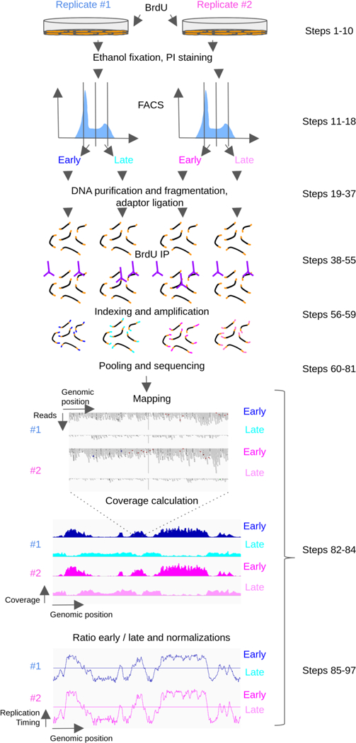
Cultured cells are pulse-labeled with BrdU, fixed and sorted into early and late S phase fractions depending on DNA content by flow cytometry. DNA from both cell fractions is purified, fragmented and adaptors are ligated. BrdU labeled DNA is immunoprecipitated, indexed and amplified. The indexed samples are pooled and sequenced. Sequenced reads are aligned on the reference genome and the normalized coverage is calculated for each cell fraction. Log ratio of early to late coverage is calculated and data are normalized and smoothed.

Labeling and fixation (Steps 1–10).

This stage is performed on cells that can be pulse-labeled, which includes any cell type that is proliferating and expresses a thymidine kinase, and that can be dissociated into single cells. Some clinical specimens can be problematic if their preservation has impaired their viability and they can no longer incorporate nucleosides. For these type of samples, we recommend either avoiding the BrdU labeling by using the S/G1 method or rejuvenation in immunodeficient mice as described in Sasaki et al.²⁰. Finally, some tissue samples may be difficult to dissociate and alternative methods of dissociation can be tried, as described³². Asynchronously proliferating cells are pulse-labeled with BrdU to mark newly synthesized DNA. The resolution of repli-seq is currently limited by the percentage of the genome that must be labeled for efficient BrdU immunoprecipitation (IP), which is approximately 10% of the genome (1 hour label minimum). Shorter labeling times result in a high proportion of unlabeled DNA contamination, increasing noise. Since eukaryotic cells replicate their genomes as spatially clustered replicons, generally large domains are labeled in a short period of time³³. The optimal concentration of nucleoside may also be affected by the cell type (e.g. endogenous nucleoside pools) or culture media. If desired, BrdU can be replaced by EdU and the pull down performed by click chemistry, but we are still optimizing the conditions for EdU labeling and the degree of improved resolution, and BrdU-IP is less expensive and faster than EdU click chemistry.

FACS sorting (Steps 11–18).

BrdU-labeled cells are stained with propidium iodide (PI) to assess the cell cycle phase of each cell. Cells are sorted by FACS according to their DNA content based on the PI staining, to isolate two cell populations: early S cells and late S cells (Supplementary Figure 1). Many other DNA staining dyes may substitute the PI (e.g. chromomycin, mithramycin, DAPI, Hoechst, DRAQ5) depending on the fluorescence wavelengths and applications desired³². We sort 20,000 cells per fraction, although we have generated good-quality data with as little as 1,000 cells (we do not recommend this for first-time users).

DNA preparation (Steps 19–24).

Early and late sorted S phase cells are lysed by SDS/Proteinase K digestion and genomic DNA is isolated using Zymo Quick-DNA purification. Theoretically, any genomic DNA preparation should work, but Zymo’s kit is designed for small amounts of DNA in small volumes. It is also fast as it does not involve pelleting and dissolving DNA.

Fragmentation (Steps 25–29).

Purified DNA is fragmented by sonication using a Covaris. The advantages of Covaris are: 1) it reproducibly fragments DNA into a relatively tight size distribution, hence there is usually no need for subsequent size selection; 2) the same conditions work for a broad range of DNA concentrations (50–5000ng). Although Covaris consumables are expensive, these advantages make the total cost of library construction lower than fragmenting DNA using other methods. The fragmentation is performed to obtain DNA fragments of an average length of 200bp if 50 to 100 bp single end sequencing is to be performed. Fragment size can be adapted for specific purposes, e.g., for experiments where we wish to detect SNPs in phased genomes, we fragment to more than 500bp fragments and perform 250bp paired end sequencing.

Library construction (Steps 30–37).

DNA libraries are constructed prior to the BrdU labeled DNA immunoprecipitation (BrdU IP), which has multiple advantages. First, the amount of available DNA is higher than after the IP and constructing libraries from small amounts of DNA is challenging. Second, BrdU IP yields single-strand DNA, which means that constructing the libraries after the BrdU IP would require converting it back to double-stranded DNA, which adds one more step to the protocol and could introduce artifacts. Importantly, this method also allows one to quantify the efficiency of the BrdU IP by quantitative PCR of IP and input DNA (see step 56 and supplementary method I). The kit used to construct the library depends on the sequencer you will use. We use an NEB kit for Illumina sequencing, which presents several advantages: 1) NEB adaptors are designed to minimize adaptor dimer formation, which is a major problem in NGS library preparation, 2) its flexibility and cost performance. This kit ligates universal adaptors to the sample and then adds an index by PCR afterwards, which permits a more flexible experiment plan, compared to, e.g., Illumina TruSeq adaptors, which are already indexed. The disadvantage of this NEB kit is that it’s impossible to detect cross-contamination and misidentification of samples that occurs before indexing. NEB’s adaptor consists of a double stranded region that is adjacent to the insert and a loop region with Uracil that is digested by the USER (Uracil-Specific Excision Reagent) enzyme after adaptor ligation to form non-homologous single-strand regions to allow annealing of directional index primers. Libraries are constructed according to the manufacturer’s instructions, following three steps: end repair and dA-tailing, adaptor ligation, and USER treatment.

BrdU Immunoprecipitation (Steps 38–55).

Adapter-ligated DNA fragments are immunoprecipitated with an anti-BrdU antibody and anti-mouse secondary antibody. The BrdU IP does not use beads to precipitate the antibody bound DNA-BrdU complexes, the centrifugation performed at Step 48 is sufficient to pellet the (always visible) complexes. However, because primary and secondary antibodies alone can make visible aggregates without BrdU-labeled DNA, visible precipitates do not guarantee successful capture of BrdU-labeled DNA.

Indexing and PCR amplification (Steps 56–59).

DNA is indexed during the PCR amplification stage, using multiplex oligos from NEB, which are designed to add the index sequence to the adaptor-ligated fragments. We use dual index for the pooling flexibility here but single index also works as far as there are enough unique indexes for the libraries to pool together, The optimum number of PCR cycles can be determined by qPCR (see step 56 and supplementary method I) if necessary.

Post-PCR Purification (Steps 60–72).

DNA is purified to remove PCR reagents, primers, primer dimers, and protein contamination. We use AMPure XP beads. As the size difference between library fragments and primer dimers is small, column-based regular PCR purification kits or ethanol precipitation are not suitable. Other size-selection kits designed for next-generation sequencing library preparation may work but we haven’t tested in our hands.

Quality Control, Pooling and Sequencing (Steps 73–81).

Quality control is an important stage to avoid sequencing low quality samples which cannot be used for further analysis. This stage includes the quantification of DNA concentration for each sample and analysis of the size distribution of the library. The performance of the BrdU-IP is assessed by semi-quantitative PCR in known early and late replicating regions, if these data are available for your samples. The supplementary methods list constitutively early and constitutively late replicating genomic loci in mouse and human genomes, hence these loci are likely to be constitutively early and constitutively late replicating in other mammalian organisms as well. If repli-seq is to be performed with a new species, one can use human or mouse cells as a positive control for the BrdU-IP performance until sufficient experience is gained with the new species to develop the appropriate regions for validation. After the quality control steps, libraries are pooled for sequencing. The pool of libraries is checked for size distribution and molar concentration before being sequenced. Sequencing is performed on a HiSeq Illumina sequencer.

Analysis (Steps 82–97).

Reads are mapped onto the genome using bowtie2. The coverage is assessed for each sample, and the base 2 log ratio of early vs. late S phase samples is calculated in genomic windows of 5 or 50kb. All analysis steps are performed using R software or in the command line. Next, base 2 log ratio files are post-processed using R. Post-processing allows the comparison between samples when comparing samples with local RT changes. Post-processing includes quantile normalization and Loess smoothing. We do not recommend using quantile normalization when comparing datasets with expected global RT changes, as it could mask the effect of global RT misregulation in samples with a massive shift in S phase read distribution, e.g. in a Rifl knockout³⁴. Loess smoothing helps noise reduction. The analysis generates one bedgraph coverage file of post-processed log2 ratio of early vs. late S phase cells per sample. These files can be viewed using a genome viewer (IG V³⁵, software.broadinstitute.org/software/igv/, IGB³⁶, bioviz.org/igb/, USCS genome browser³⁷, genome.ucsc.edu/), but we recommend using the replicationdomain platform (www.replicationdomain.org), which allows comparison to our database of hundreds of available RT, genome-wide transcription and 4C datasets³⁸. Moreover, the Bedgraph files can be easily integrated into further analysis pipelines e.g. comparison with other RT datasets or chromatin marks.

MATERIALS

REAGENTS

CRITICAL All reagents/materials should be molecular biology / PCR grade.

- Cells of interest (here we are using F121–9 mouse hybrid ES cells³⁹ and RCH-ACV lymphoblastoid cells (DSMZ ACC 548); see REAGENTS SETUP)

CAUTION: The cell lines used in your research should be regularly checked to ensure they are authentic and are not infected with mycoplasma.

- BrdU (Sigma-Aldrich, cat. no. B5002)

CRITICAL Protect from light.

- Cell culture medium and FBS appropriate for the cell type (N2B27 2i LIF used for F121–9 (Cold Spring Harbor Protocols, PMID:28461676), RPMI 1640 (Corning, cat. no. 10040CV) + 10% heat-inactivated FBS (Seradigm, cat. no. 1500–500H) for RCH-ACV)

- 1× Trypsin-EDTA (Mediatech, cat. no. 25–053-Cl) or other cell dissociation reagent appropriate for the cell type

- 1× PBS (Corning, cat. no. 21–031-CV)

- Propidium Iodide (PI) (Sigma-Aldrich, cat. no. P4170-)

CRITICAL Protect from light.

CAUTION PI is a DNA chelator, were gloves to manipulate it or any solution that contains PI.

- RNase A 20mg/mL (Sigma-Aldrich, cat. no. R6148) CRITICAL: Store at 4°C

- Proteinase K 20mg/mL (Amresco, cat. no. E195) CRITICAL:Store at 4°C

- SDS (Invitrogen, cat. no. 15525017)

- Quick-DNA MicroPrep (Zymo, cat. no. D3021)

- 0.5 M EDTA pH 8 (Boehringer, cat. no. 808288)

- Sodium Chloride (Mallinckrodt, cat. no. 758119)

- NEBNext Ultra DNA Library Prep Kit for Illumina (cat. no. E7370)

- TE (Sigma, cat. no. 93283, or homemade: 10 mM Tris pH 8.0, 1mM EDTA)

- 10 mM Tris pH 8.0 (Teknova, cat. no. T1173)

- HCl (Sigma-Aldrich, cat. no. H1758)

- Sodium Phosphate (Sigma-Aldrich, cat no. S3264)

- Triton X100 (Sigma-Aldrich, cat. no. T-9284)

- Anti-BrdU antibody (BD, cat. no. 555627)

- Anti-mouse IgG (Sigma-Aldrich, cat. no. M7023)

- NEBNext Multiple Oligos for Illumina (Dual Index Primers Set 1, cat. no. E7600S)

- DNA Clean & Concentrator-5 (Zymo Research, cat. no. D4014)

- Agencourt AMPure XP (Beckman Coulter, cat. no. A63880)

- Qubit® dsDNA HS Assay Kit (Life Technologies, cat. no. Q32854)

- Agilent High Sensitivity DNA Kit (Agilent, cat. no. 5067–4626)

- Agilent DNA 1000 Kit (Agilent, cat. no. 5067–1504)

- 100% (vol/vol) Ethanol (Sigma-Aldrich, cat. no. E7023)

- H₂O (any molecular biology / PCR grade, typically, autoclaved distilled water)

- Tween 20 (Sigma-Aldrich, cat. no. P1379)

- KAPA Library Quantification kit (Kapa biosystems, cat. no. KK4824 for Applied Biosystems 7500 Fast)

- Tris HCl pH 8 (ThermoFisher, cat. no.15568025)

- EtBr (Fisher Scientific, cat. no. BP102–5) CAUTION Ethidium bromide is a mutagen and potential carcinogen; handle it with care.

EQUIPMENT

- Covaris E220

- microTUBE AFA Fiber Pre-Slit Snap Cap 6×16mm (Covaris, cat. no. 520045)

CRITICAL Tubes are single use. They are used with Covaris rack (cat. no. 500111)

- heat block

- Qubit

- Centrifuge (Eppendorf, cat. no. 5415D and Sorvall Legend RT)

- Magnet separator (NEB, cat. no. S1509S)

- Thermal cycler (with plate for 0.5mL tubes)

- 1.5mL low bind microcentrifuge tubes (e.g. USAScientific, cat. no. 1415–2600)

- 0.5mL PCR tubes (we use Axygen, cat. no. PCR-05-C, but exact tubes have to be adapted to your thermal cycler)

- 0.65mL microcentrifuge tubes (Coster, cat. no. 3208)

- Real-Time Thermocycler (Applied Biosystems 7500 Fast)

- PCR plate (Life Technologies, cat. no. 4346906)

- Optical Adhesive Film (Life Technologies, cat. no. 4311971)

- Parafilm

- 15 mL round bottom tube (Falcon, cat. No. 2059)

- 37-micron nylon mesh (Small Parts, cat. no. CMN-0040-D/5PK-05, Amazon.com, alternatively Coring, cat no. 352235)

- 5 mL polypropylene round bottom tube (Corning, cat no. 352054)

- Bioanalyzer High Sensitivity DNA chip (Agilent Technologies, cat. no 5067–4626)

- Vortex

- Unix-based Computer with at least 4 cores, 16GB memory and 200GB of hard disk space

Software

- R⁴⁰ (https://www.r-project.org/)

- R package “preprocessCore”⁴¹ (bioconductor.org)

- R package “travis” (Optional) (Doi: 10.5281/zenodo.269005; https://github.com/dvera/travis)

- fastqc (Andrews S. (2010). FastQC: a quality control tool for high throughput sequence data. http://www.bioinformatics.babraham.ac.uk/projects/fastqc)

- bowtie2⁴² (Bowtie2 needs the index of the genome you will use, http://bowtie-bio.sourceforge.net/bowtie2/index.shtml)

- samtools⁴³ (http://www.htslib.org/download/)

- bedtools⁴⁴ (http://bedtools.readthedocs.io/en/latest/index.html)

REAGENTS SETUP

- Cells of interest

Cultures can be grown in any size cell culture dish, but must be in an actively dividing state for use in this protocol. If you have to start from frozen samples that were proliferating at the time they were frozen but are no longer metabolically active, use the S/G1 method described by Ryba et al¹⁸. Since FACS can be problematic with a low cell number, we recommend starting with greater than 2 × 10⁶ cells. We have successfully profiled RT using as low as 300,000 starting cells, and as few as 1000 early and late S phase cells after sorting, but cells are lost during PI staining, filtering, sorting so we do not recommend trying this without extensive experience.

CAUTION: All experiments should be performed in accordance with relevant health, safety and human subjects guidelines and regulations.

- BrdU (5-bromo-2’-deoxyuridine)

Make stock solutions of 10 mg/mL (and 1 mg/mL if you need to handle a small scale of culture) in ddH2O (warm up in 37°C water bath to dissolve completely) and store at −20°C in 1mL aliquots aliquots, protected from light. Aliquots can be stored for more than 2 years. Repeated freeze / thaw is fine.

-Propidium Iodide (1 mg/mL) (PI)

To make 20 mL, dissolve 20 mg Propidium Iodide powder in autoclave ddH₂O to achieve a final volume of 20 mL and filter. Store for up to one year at 4°C protected from light. 1mL aliquots are convenient.

- PBS / 1% (vol/vol) FBS / PI / RNase A

Add 50 μl of 1 mg/ml PI, 12.5 μl of 20 mg/ml Rnase A to every 1 ml of PBS-1% (vol/vol) FBS. PBS / 1% (vol/vol) FBS / PI / RNase A should be prepared each time and not to be stored. FBS can be stored at −20°C in aliquots.

- 1M Tris-HCl pH 8.0

Dissolve 121.14 g Tris in 800 ml dH₂O. Adjust pH to 8.0 with the appropriate volume of concentrated HCl. Bring final volume to 1 liter with deionized water. Autoclave and store at room temperature (25°C), indefinitely. Alternatively, buy ThermoFisher, cat. no.15568025.

- 1M Sodium Phosphate pH 7.0

Solution A: Dissolve 138.0 g NaH2PO4-H2O in 1 liter dH2O (pH 7.0). Solution B: Dissolve 142.0g Na2HPO4 in 1 liter dH2O (pH 7.0). Mix 423 ml Solution A with 577 ml Solution B. Autoclave and store at room temperature, indefinitely, as far as it is not contaminated.

-SDS-PK buffer

To make 50 mL, combine 34 mL autoclaved ddH₂O, 2.5 mL 1M Tris-HCl pH 8.0, 1 mL 0.5 M EDTA, 10 mL 5 M NaCl and 2.5 mL 10% (wt/vol) SDS in H₂O. Store at room temperature, indefinitely. Warm to 56°C before use to completely dissolve SDS.

- 10× IP buffer

To make 50 mL, combine 28.5 mL ddH₂O, 5 mL 1M Sodium Phosphate pH 7.0, 14 mL 5 M NaCl, and 2.5 mL 10% (wt/vol) Triton X-100 in H₂O. Store at room temperature, indefinitely.

- anti-BrdU antibody 12.5 μg/ml

Dilute antibody in 1× PBS from the stock concentration of 0.5 mg/mL to a final concentration of 12.5 μg/mL. Prepare 40 μl of diluted antibody for each sample. Diluted antibody should be used on the same day and should not be saved.

- Digestion buffer

To make 50 mL, combine 44 mL autoclaved ddH₂O, 2.5 mL 1M Tris-HCl pH 8.0, 1 mL 0.5 M EDTA, and 2.5 mL 10% (wt/vol) SDS in H₂O. Store at room temperature, indefinitely.

- NEBNext Ultra DNA Library Prep Kit for Illumina (E7370)

The Ligation Master Mix and Ligation Enhancer can be mixed ahead of time and the mix is stable for at least 8 hours at 4°C. We do not recommend premixing the Ligation Master Mix, Ligation Enhancer and adaptor prior to use in the Adaptor Ligation Step.

PROCEDURE

BrdU pulse labeling and fixation of cells 3h

CRITICAL: Starting from rapidly growing cells helps as they have a large percentage of S phase cells. In our experience, 2 million total cells, with >5% cells in S phase, yields enough early and late S phase cells for one replication assay (60,000 each).

CRITICAL: The following steps are for adherent cells in a T75 flask with 15 mL of medium. For cells in a 15mL suspension culture, skip steps 3 to 5).

1. Add BrdU into medium to a final concentration of 100 μM

2. Incubate 2 hr at 37°C in a tissue culture incubator for BrdU incorporation

3. Gently rinse the cells twice with ice-cold PBS

4. Trypsinize the cells with 2 mL of 0.2× Trypsin-EDTA for 2–3 min (incubation temperature varies depending on the cell line used, please refer to the provider. Here, F121–9 are trypsinized at RT)

5. Add 5 mL of complete medium, pipette gently but thoroughly, and transfer to a 15 mL round bottom tube.

CRITICAL STEP Using round bottom tubes for cell fixation prevents cells from forming packed pellet that is hard to re-suspend later, but if small cell number is an issue, using conical tubes is fine.

6. Centrifuge the cells at 200 g for 5 min at RT

7. Decant (or aspirate) supernatant carefully

8. Add 2.5 mL of ice-cold PBS / 1 % (vol/vol) FBS, pipette gently but thoroughly

CRITICAL STEP Double check the cell number using a hemocytometer or any cell counter at this point. After adding ethanol it will be harder to count cells since FBS deposits as a sediment on addition of ethanol.

9. Add 7.5 mL of ice-cold 100% (vol/vol) EtOH, dropwise while gently vortexing

CRITICAL STEP Use the lowest rpm or hand shake the tube to avoid cell lysis by vigorous vortexing

10. Seal the cap and mix the tube gently but thoroughly by inverting several times and store at −20 until use.

PAUSE POINT Fixed cells are stable at −20°C for more than a year if protected from light (BrdU is light sensitive) and evaporation. Lower temperature may cause freezing which damages cells.

CRITICAL STEP: Starting from rapidly growing cells helps as they have a large percentage of S phase cells. In our experience, 2 million total cells, with >5% cells in S phase, yields enough early and late S phase cells for one replication assay (60,000 each).

FACS sample preparation and sorting 1.5h

CRITICAL: The following steps describe the procedure for sorting whole, single cells. If condition of the fixed cells is poor, e.g. many cell aggregates in the suspension, or if the cell sorter does not allow sorting whole cells, e.g. due to a too narrow nozzle, the “nuclei preparation” procedure (see Supplementary method II.) can be used.

11. Transfer 2 × 10⁶ cells from Step 10 to a new 15 mL conical tube.

12. Centrifuge at approximately 200 × g for 5 minutes at room temperature and decant the supernatant carefully

13. Resuspend the cell pellet in 2 mL 1% (vol/vol) FBS in PBS. Mix well by tapping the tube.

14. Repeat Step 12

15. Resuspend cell pellet in 0.5mL PBS / 1% FBS / PI / RNase A aiming to reach a final concentration of 3 × 10⁶ cells/mL.

16. Tap the tube to mix and then incubate for 20 to 30 minutes at room temperature (25°C) in the dark. (count the cells during this time and adjust cell concentration to 3 × 10⁶ cells/mL by either adding more PBS / 1% FBS / PI / RNase A or centrifuging, removing the supernatant and resuspending the pellet in an appropriate volume if necessary)

17. Filter the cells by pipetting them through 37-micron nylon mesh into a 5 mL polypropylene round bottom tube. Keep samples on ice in the dark and proceed directly to FACS sorting.

PAUSE POINT Alternatively, add 1/9 vol. DMSO and freeze at −80°C (light protected) until sorting. Frozen cells can be stored indefinitely. On sorting, thaw the cell suspension in a 37°C water bath and keep the samples on ice in the dark. Removing the DMSO is not necessary.

18. Collect 120,000 early and 120,000 late S phase cells by FACS sorting.(120,000 cells allow 6 reactions of BrdU IP).

See Supplemental Figure 1 for sorting gate specifications.

TROUBLESHOOTING

DNA preparation from FACS sorted cells 3h

19. Centrifuge the sorted cells at 400 × g or sorted nuclei at 800 × g for 10 minutes at 4°C.

20. Decant supernatant gently, only once (If the cell number is small, there may be no supernatant coming out by decanting).

21. Add 1 mL of SDS-PK buffer containing 0.2 mg/mL Proteinase K to every 100,000 cells collected (Although we aim to collect 120,000 cells/fraction, “early S” and “late S” fractions do not always have the same number of cells. The cell sorter keeps collecting cells until both “early S” and “late S” fractions have at least 120,000 cells. Alternatively, one may end up with less than 120,000 cells due to a low S phase population. In those cases, add 1 mL buffer to every 100,000 cells to adjust the cell concentration.) and mix vigorously by tapping the tube. Seal the tube cap with parafilm to prevent them from popping off during Step 22.

22. Incubate the samples in a 56°C water bath for 2 hours.

23. Mix each sample thoroughly to get a homogeneous solution, then aliquot 200 μl, equivalent to approximately 20,000 cells, into separate 1.5 mL tubes for each sample. (One tube is for one library/IP. In order to see the consistency of IP, it is recommended to process at least 2 fractions per sample).

24. Add 800 μl Genomic Lysis Buffer from the Zymo Quick-DNA Microprep kit and purify the DNA following the manufacturer’s instructions. Elute the DNA into 50 μl H2O.

CRITICAL STEP Pay great attention to make sure you do not have wash buffer left on the column before adding 50 μl H2O for elution.

PAUSE POINT The purified DNA can be sheared immediately or stored in −20°C indefinitely.

Fragmentation 1h

CRITICAL The Covaris water bath needs to be chilled at 4–7°C and de-gassed for 45 minutes before each use. See the manufacturer instructions for more information.

25. Using a 100–200 μl pipette tip, transfer the purified DNA from Step 24 into a microTUBE AFA Fiber (numbered on periphery of the cap) through the slit of the microTUBE (the slit closes automatically). Keep the tube containing on ice until fragmentation starts.

26. Place the sample tubes on the rack and sonicate the DNA as follows for a 200 bp average fragment size: 175W, 10% duty cycle, 200 cycles/burst, 120 seconds and 4–7°C water bath temperature.

28. Once all tubes have been sonicated, spin the tubes at 600 g for 5 sec using the adaptors provided by Covaris to collect all the liquid at the bottom of the tube.

29. Optional: Although Covaris is very reproducible, you may want to check the fragment size distribution, especially on your first try. Concentrate the sheared DNA to 10–15 μL using DNA Clean & Concentrator-5 and check 1 μL on a Bioanalyzer High Sensitivity DNA chip.

Library construction 3h

CRITICAL After each step, purified DNA can be stored in −20°C indefinitely. Pausing after enzyme reaction without DNA purification is not recommended. We perform all the enzyme reactions in 0.5mL PCR tubes using a thermal cycler equipped with heat blocks for 0.5mL tubes for convenience (0.5mL tubes can hold these relatively large volumes of reactions as well as DNA purification afterwards can be done in the same tube). If you do not have an access to a thermal cycler equipped with heat blocks for 0.5mL tubes, reactions can be divided into multiple smaller PCR tubes.

30. Prepare the following mix in a 0.5ml PCR tube:

Component	Amount	Final concentration
End Prep Enzyme Mix	3μL	1×
End Repair Reaction Buffer 10×	6.5μL	1×
Fragmented DNA from Step 28+ H2O	55.5μL	7.7 ng/mL to 15.4 μg/mL
Total Volume	65μL

31. Mix by pipetting followed by a quick spin to collect all liquid from the sides of the tube.

32. Place in a thermocycler, after the lid is heated to 105 °C, and run the following program.

Duration	Temperature
30 minutes	20°C
30 minutes	65°C
Hold	4°C

33. Add the following components directly to the mix from Step 32 and mix well by pipetting up and down, followed by a quick spin to collect all liquid from the sides of the tube.

Component	Amount	Final concentration
Mix from step 32	65μL	1×
Blunt/TA Ligase Master Mix	15μL	1×
NEBNext Adaptor for Illumina	2.5μL	0.45μM
Ligation Enhancer	1μL	1×
Total Volume	83.5μL

CRITICAL STEP If you started with less than 100 ng DNA, dilute the NEBNext Adaptor 1:10 with H2O. Diluted adaptor cannot be saved for later use, so discard any leftover.

34. Incubate at 20°C for 15 minutes in a thermal cycler with heated lid off.

35. Add 3μl USER enzyme to the ligation mixture and mix well by tapping.

36. Incubate at 37°C for 15 minutes with heated lid (50°C) on.

37. Purify the DNA using DNA Clean & Concentrator-5, following the manufacturer’s instructions. Elute in 50 μl H₂O.

PAUSE POINT The purified DNA can be stored indefinitely at −20°C protected from light.

BrdU IP 1h and overnight

38. Add 450 μL TE to the DNA from Step 37.

39. Aliquot 60 μL 10× IP buffer to separate fresh 1.5mL tubes (one for each sample from Step 38).

40. Prepare 0.75 mL 1× IP buffer for each sample and start cool on ice.

41. Denature the DNA from Step 38 at 95°C for 5 minutes then cool on ice for 2 minutes. Briefly spin to collect any condensation on the tube cap to the bottom of the tube.

42. Add the denatured DNA from Step 41 to the prepared tubes with 10× IP buffer from Step.

43. Add 40 μL of 12.5 μg/mL anti-BrdU antibody to each tube.

44. Incubate 20 minutes at room temperature with constant rocking.

46. Add 20 μg of rabbit anti-mouse IgG.

CRITICAL STEP Anti-mouse IgG concentration differs lot by lot. Check certificate of analysis for concentration details.

47. Incubate 20 minutes at room temperature with constant rocking.

48. Centrifuge at 16,000 × g for 5 minutes at 4°C and remove the supernatant.

49. Briefly spin the samples and remove the remaining supernatant, first using 200 μL tips, followed by10 μL tips).

CRITICAL STEP Make every effort to completely remove the supernatant

50. Add 750 μL of the chilled 1× IP Buffer from Step 40.

51. Repeat Steps 48 and 49.

52. Re-suspend the pellet in 200 μL digestion buffer with freshly added 0.25 mg/mL Proteinase K and incubate samples overnight at 37°C in an air incubator. (NOTE: If you do this in a water bath, water in the reaction evaporates and makes condensation under the cap during the overnight incubation, leaving almost no solution at the bottom of the tube.)

53. Add 1.25 μL of 20 mg/ml Proteinase K to each tube.

54. Incubate samples for 60 minutes at 56°C (water bath or heat block).

55. Purify the DNA using DNA Clean & Concentrator −5, following the manufacturer’s instructions. Elute the purified DNA in 16 μL H2O.

PAUSE POINT The purified DNA can be stored indefinitely at −20°C protected from light.

Indexing and amplification 1.5h

56. (Optional) In order to estimate the DNA yield of your BrdU-IP and determine the optimal PCR cycle number for indexing, perform a qPCR using primers that anneal to adaptor(in this case: NEBadqPCR_F; ACACTCTTTCCCTACACGACGC and NEBadqPCR_R; GACTGGAGTTCAGACGTGTGC) and serial dilution of your previous NGS library with known concentration as standard (see supplementary method I).

57. Mix the following components in a 0.5mL PCR tubes, one for each sample from Step 55.

CRITICAL STEP See Supplementary Data I for more information on NEBNext primers, and refer to NEB and Illumina manuals on how to combine index primers.

Component	Amount	Final concentration
BrdU IP library from step 55	15μL	1×
NEBNext Q5 Hot Start HiFi Master Mix	25μL	1×
i7 Primer	5μL	1μM
i5 Primer	5μL	1μM
Total Volume	50μL

CRITICAL STEP Each library should get a unique combination of i7 and i5 primers.

58. Place in a thermocycler, after lid is heated to 105°C, and run the following PCR program:

Cycle Number	Denature	Anneal	Extend	Hold
1	98°C, 30s
2–15	98°C, 10s	65°C, 75s
16			65°C, 5min
17				4°C

CRITICAL STEP The necessary number of cycles varies depending on the yield of the BrdU IP. If the suggested cycle number is not enough, you can re-amplify your libraries after Step 72 according to Box 1. Re-amplification skipping PCR purification often causes primer dimer amplification hence not recommended). Over-amplification with primer depletion causes PCR artifacts and should be prevented

Box 1. Reamplification Procedure.

1. Mix the following components in a 0.5mL PCR tube:

Component	Amount	Final concentration
Indexed library from Step 72	20μL	1×
TS-Oligo 1&2 (6μM each)	5μL	0.6μM each
NEBNext Q5 Hot Start HiFi Master Mix	25μL	1×
Total volume	50μL

CRITICAL STEP TS-Oligo 1&2 anneal to the outermost part of indexed (both dual and single indexed) library molecules. This primer set cannot be used before library indexing. Sequences of the oligosan be found in Supplementary Data II.

2. Place the mix in a thermocycler, after lid is heated, and run the following program:

Cycle Number	Denature	Anneal	Extend	Hold
1	98°C, 30s
2 - as needed	98°C, 10s	65°C, 75s
Final extension			65°C, 5min
Hold				4°C

CRITICAL STEP The PCR program is basically the same as for indexing (Step 58) but cycle number is adjusted depending on the original template concentration. Our equipment and this primer set amplify DNA approximately 1.7 times per cycle (this could vary depending on the thermal cycler). In addition, 60–70% of PCR product will be lost during post-PCR purification. Altogether, use 10 cycles for 100 fold amplification, 6–7 cycles for 10 fold amplification, or 4–5 cycles for 3 fold amplification.

CRITICAL STEP Avoid over-amplification, to prevent library dimer, trimer, etc. formation.

3. Purify the PCR product and quantify DNA using Qubit as performed in Steps 60 to 73.

59. (Optional) Run 5uL of each PCR reaction on a 1.5% (wt/vol) agarose gel to check the size distribution by EtBr staining (see Lee et al.⁴⁵ for more information about gel electrophoresis). A smear around 350 bp is expected. If no smear is detected, you need to re-amplify the reaction (the procedure for re-amplification is described in Box 1).

Purificationa 1h

60. Place AMPure XP beads at room temperature for at least 30 minutes.

61. Add H₂O to each PCR reaction to make the final volume 100uL.

62. Vortex AMPure XP beads to resuspend.

63. Add 90μL of resuspended AMPure XP beads to the 100μL PCR reaction. Mix well by pipetting up and down at least 10 times.

CRITICAL STEP If you start from poorly fragmented DNA and you are sure you need to perform size selection at this moment, refer to NEB manual E7370 and optimize the volume of AMPure XP beads to use. Briefly, save the supernatant from the first selection to remove larger fragments which bind to the beads, then add more\ AMPure XP beads to bind the fragments of target size and discard the supernatant this time, wash the beads with 80% ethanol as Steps 66–69 and elute the target size fragments from the beads as Step 70.

64. Incubate for 5 minutes at room temperature.

65. Freshly prepare 600 μL 80% (vol/vol) ethanol per sample by diluting 100% ethanol with H₂O

66. Quickly spin the tubes from Step 64 in a microcentrifuge and place the tube on a magnetic stand to separate the beads from the supernatant. Once the solution is clear (about 5 minutes), carefully remove the supernatant.

67. Add 200 μL 80% (vol/vol) freshly prepared ethanol from Step 65 to each tube while in the magnetic stand. Incubate at room temperature for 30 seconds, and then carefully remove and discard the supernatant.

68. Repeat Steps 66–67 two more times for a total of three washes.

69. Briefly spin the tubes in a microcentrifuge and remove the residual 80% ethanol. Air dry the beads for 10 minutes while the tube is on the magnetic stand with the lid open but loosely covered by plastic wrap.

70. Elute the DNA from the beads by adding 33 μL 10 mM Tris-HCl. Mix well on a vortex mixer or by pipetting up and down.

71. Quickly spin the tubes in a microcentrifuge and return them to the magnetic stand.

72. Once the solution is clear (about 5 minutes), transfer 31 μL to a new tube. Store libraries at – 20°C until use.

CRITICAL STEP Make sure not to disturb the magnetic beads or take up any beads when transferring the elution. If your supernatant still contains beads, repeat Step 71 and remove the beads from the supernatant completely.

PAUSE POINT DNA libraries can be stored indefinitely at −20°C

Quality control and pooling 5h

73. Check the DNA concentration using 1 μL of the library from Step 72 on a Qubit dsDNA HS Assay Kit, following the manufacturer’s instructions. A DNA yield of10–20 ng/μl is expected. If the concentration is below the detection limit, do another Qubit assay using 10 μL of DNA library. This helps to determine the number of PCR cycles necessary for re-amplification.

CRITICAL STEP If the DNA concentration is less than 7 ng/μl, you will have problems making the final 10 nM pool, so you will need to re-amplify the sample. Please note that it is better to use more PCR cycles at Step 58 rather than re-amplifying, because re-amplification increases the risk of bias by PCR as well as includes one more step of purification which costs more, is timeconsuming, and could be another source of bias. Re-amplification can be done by following the procedure described in Box 1.

TROUBLESHOOTING

74. If your sample is from mouse or human using 2 ng/μL dilutions of each library as templates, check the early and late fraction enrichment by following the supplemental procedure described in Box 2, using primer sets listed by Ryba et al.¹⁸. See Supplementary Table 1 for combination of Multiplex Primers. If the expected target enrichment is confirmed, proceed to Step 75.

Box 2. Early over late fraction enrichment validation in Human and Mouse.

1. Mix the following components in a 0.2 ml PCR tube:

Component	Volume per reaction (μl)	Final concentration
ddH2O	1.25 μl	-
2×One Taq master mix (NEB M0486)	6.25 μl	1×
Multiplex Primer mix	4 μl	various
Template 2 ng/μL diluted from an aliquot from Step 72	1 μl	0.16 ng/μl
Total	12.5 μL

2. Place the mix in a thermocycler with the program pausing, after the heat block is heated to >90°C° (this polymerase is not hot start), and run the following program:

Cycle Number	Denature	Anneal	Extend	Hold
1	95°C, 30s
2–40	94°C, 20s	60°C, 45s
41			65°C, 5min
42				4°C

CRITICAL STEP Since the target size is small enough, this 2-step PCR works without an extension step. However, it is important to stick to this annealing condition (45s is relatively long) so that the primer can start extension slowly during the annealing instead of suddenly being stripped from the template by heating for the next cycle of denaturation.

3. Run 4–5 μL of each PCR product (addition of loading buffer is not necessary for One Taq PCR) on 1.5% (wt/vol) agarose gel containing 0.1 μ/.mL EtBr to separate 150–450 bp in your gel system to check the size of PCR products (specificity of PCR) and target enrichment. Each PCR product is from either “a typical early replicating locus” or “a typical late replicating locus” hence should be enriched in either the “early S” library or “late S” library.

TROUBLESHOOTING

75. Following the manufacturer’s instructions, check the size distribution of each library from Step 72 using the Bioanalyzer high sensitivity DNA kit or DNA 1000 kit, depending on the DNA concentration measured at Step 73. See Supplementary Figure 2 for examples of good and bad quality libraries.

A good DNA library contains no adaptor/primer dimer peaks (below 150–180 bp) (primer dimers contribute to invalid sequencing reads). It is also important that all the libraries to be pooled have a similar and tight (~ 300 bp width) size distribution. (Molecules of different size have different clustering efficiency during sequencing). If your samples do not meet these criteria, go back to Step 60. If all your samples pass these criteria, proceed to Step 76

76. (Optional) Determine of the molar concentration of each library by qPCR. This step may be omitted after you get used to the procedure. See manufacturer’s instruction for the latest update on the KAPA qPCR kit. If your library has an average size of 350 bp and a concentration of 10ng/uL, the molar concentration is around 50nM, hence 1:10,000 dilution would fit within the standard curve. Set up triplicates of standard DNA and duplicates of test samples (decide the dilution factor based on your Qubit and Bioanalyzer results).

After the PCR run, calculate the molar concentration of your samples, using the average fragment size from Bioanalyzer as follows:

$$MolarConcentration\left(nM\right)=RawMolarConcentration\left(nM\right)*452\left(bp\right)/AvFragSize\left(bp\right)$$

Where RawMolarConcentration is the raw molar concentration obtained by qPCR and AvFragSize your average fragment size. 452 is the size of the standard DNA fragments used by the KAPA Illumina library quantification assay kit.

77. Pool the libraries. Using 0.05 % (vol/vol) Tween 20 in 10 mM Tris pH 8, adjust each library to 10 nM (if you skipped Step 76, estimate the molar concentration of each library using the Bioanalyzer’s region function).

CRITICAL STEP: The number of libraries to pool is important to reach a good sequencing depth. For human or mouse samples, 5M mapped reads per library gives usable data, which correspond to approximately 10M sequenced reads (depending on the quality of the sequencing). Our HiSeq2500 generates ~160M reads per lane, so we usually pool 12 to 16 libraries per lane. Pooling less than 4 indexes is not recommended due to the low complexity of the index.

78. Mix equal volumes of each 10 nM library to make a pool. One pool fills one sequencing lane.

CRITICAL STEP Consult your sequencer operator regarding minimal sample concentration and volume.

PAUSE POINT The DNA library pool can be stored at −20°C indefinitely.

80. Quality control of the pool(s). Take 1 μL from each pool and quantify it on a Qubit as in Step 73. Adjust the concentration to 0.5 ng/μL. Run 1 μL of each pool on a Bioanalyzer DNA HiSensitivity chip to determine the average fragment size of the pool, this should be ~350bp.

81. Sequence the pooled libraries on a Hi-seq Illumina sequencer. Generally, 50bp single-end reads is sufficient for normal samples covering the unique sequences of the genome. However, longer reads may be required to parse alleles by SNPs.

Data Analysis 1 day

CRITICAL Data analysis is performed on fastq or fastq.gz files, and outputs genomic coverage files with the log ratio of early versus late S phase samples. This pipeline is written to process files with names that follow a specific nomenclature: early and late sequencing data originated from the same sample must have matching name, with an “_E_” before the extension of the file from early S cells, and an “_L_” before the extension of the file from late S cells. If you use paired-end sequencing data, paired files must be named with R1 and R2 before the extension. An example of a single-end fastq file name could be “my_sample_1_E_.fastq” and “my_sample_1_L_.fastq”. Paired-end fastq files name could be “my_sample_1_E_R1.fastq” for read 1 and “my_sample_1_E_R2.fastq” for read 2 of the same fraction. You can also directly use a similar pipeline available on https://github.com/dvera/shart.

82. Control the quality of the reads using fastqc according to the instructions provided here:. http://www.bioinformatics.babraham.ac.uk/projects/fastqc

TROUBLESHOOTING

83. Open a shell, go to the fastq files directory and generate the windows file. Replace “path/to/files” in bold by the path to the fastq files directory, “your genome.chrom.sizes” in bolt by the chrom.sizes file name (and path, if the file is not in your working directory). You can also change the window size, and step by replacing the bold “50000” by the desired sizes in kb. Depending on the further analysis performed on the RT datasets, we use genomic windows from 5 to 50kb.

CRITICAL STEP This step requires the chrom.sizes file of the genome you will you use for the analysis. Many of these files can be directly downloaded from UCSC server at ftp://hgdownload.cse.ucsc.edu/goldenPath/. This file contains two columns: one with the chromosome name and one with its size in bp, separated by a tabulation. This file must be sorted on the first column, following alphabetic order (e.g. “chr10” will be before “chr2”).

$ cd path/to/files/
$ sort -k1,1 -k2,2n your_genome.chrom.sizes > your_genome_sorted.chrom.sizes
$ bedtools makewindows -w 50000 -s 50000 -g your_genome_sorted.chrom.sizes > your_genome_windows.bed

84. Process the fastq files. If you have multiple fastq files per libraries, see Supplementary Method III to concatenate the fastq files. See Supplementary Method IV to generate log ratio coverage files using R, and supplemental method V to map the reads on two genomes and generate the log ratio coverage files for each genome using R.

CRITICAL STEP Paths and names have to be adapted to the path and names used in your computer. For more information on the genome path used by bowtie2 and others bowtie2 options, see http://bowtie-bio.sourceforge.net/bowtie2/manual.shtml. For better performance, you can allow bowtie2 multiple processors, depending on your resources, with the option -p [number of processors] (see bowtie2 documentation). If reads quality is bad at the end of the reads, you can trim the reads with bowtie2 option --trim3.

(A) If you are analysing single-end data

(i) $ for file in *.fastq*; do
bowtie2 -x path_to_your_genome --no-mixed --no-discordant --reorder -U $file -S ${file %.fastq*}.sam 2>> ${file%.fastq*}_mapping_log.txt
samtools view -bSq 20 ${file%.fastq*}.sam > ${file%.fastq*}.bam
samtools sort -o ${file%.fastq*}_srt.bam ${file%.fastq*}.bam
samtools rmdup -S ${file%.fastq*}_srt.bam ${file%.fastq*}_rmdup.bam
bamToBed -i ${file%.fastq*}_rmdup.bam | cut -f 1,2,3,4,5,6 | sort -T . -k1,1 -k2,2n -S 5G > $ {file%.fastq*}.bed
x=‘wc -l ${file%.fastq*}.bed | cut -d’ ‘-f 1’
bedtools intersect -sorted -c -b ${file%.fastq*}.bed -a your_genome_windows.bed | awk -vx=$x ‘{print $1,$2,$3,$4*1e+06/x}’ OFS=‘\t’ > ${file%.fastq*}.bg
done
(ii) $ for file in *_E_.bg; do
paste $file ${file%E_.bg}L_.bg | awk ‘{if($8 != 0 && $4 != 0){print $1,$2,$3,log($4/$8)/log(2)}}’ OFS=‘\t’ > ${file%E_.bg}T_.bg
done
(iii) (A) if you have only one sample
 (i) $ cp *T_.bg merge_RT.txt
(B) If you have multiple samples
 (ii) bedtools unionbedg -filler “NA” -i *T_.bg > merge_RT.txt

(B) If you are analysing paired-end data

(i) $ for file in *R1.fastq*; do
bowtie2 -x path_to_your_genome --no-mixed --no-discordant --reorder -X 1000 −1 $file −2 ${file%R1.fastq*}R2.fastq* -S ${file%R1.fastq*}.sam 2>> ${file %R1.fastq*}mapping_log.txt
 samtools view -bSq 20 ${file%R1.fastq*}.sam > ${file%R1.fastq*}.bam
 samtools sort -o ${file%R1.fastq*}_srt.bam ${file%R1.fastq*}.bam
 samtools rmdup -S ${file%R1.fastq*}_srt.bam ${file%R1.fastq*}_rmdup.bam
 bamToBed -i ${file%R1.fastq*}_rmdup.bam | cut -f 1,2,3,4,5,6 | sort -T . -k1,1 -k2,2n -S 5G > ${file%R1.fastq*}.bed
 x=‘wc -l ${file%R1.fastq*}.bed | cut -d’ ‘-f 1’
 bedtools intersect -sorted -c -b ${file%R1.fastq*}.bed -a your_genome_windows.bed | awk -vx=$x ‘{print $1,$2,$3,$4*1e+06/x}’ OFS=‘\t’ > ${file%R1.fastq*}.bg
done
(ii) $ for file in *_E_.bg; do
 paste $file ${file%E_.bg}L_.bg | awk ‘{if($8 != 0 && $4 != 0){print $1,$2,$3,log($4/$8)/log(2)}}’ OFS=‘\t’ > ${file%E_.bg}T_.bg
done
(iii) (A) if you have only one sample
 (i) $ cp *T_.bg merge_RT.txt
(B) If you have multiple samples
 (ii) bedtools unionbedg -filler “NA” -i *T_.bg > merge_RT.txt

CRITICAL STEP: Mapping issues or aneuploidy will affect the final RT data. You can look at the coverage by plotting .bam files in your genome viewer to monitor the coverage on a local region. You can also monitor the global percentage of mapped reads (it should be superior to 60% of the reads) in the .log files generated by this pipeline to identify general mapping issues. Finally, aneuploidy issues can be detected as we previously described²⁸.

85. Post-process the bedgraph files in R. Open R and load the “preprocessCore” package using the following command:

> library(preprocessCore)

86. Go to the directory containing the bedgraph files and import them into R, by running the following commands:

> setwd(“path/to/files/”)
> merge<-read.table(“merge_RT.txt”, header=FALSE)
> colnames(merge)<-c(c(“chr”,”start”,”end”),list.files(path=“.”,pattern=“*T_.bg”))
> merge_values<-as.matrix(merge[,4:ncol(merge)])

87. Set the datasets to use for quantile normalization by using the following commands (bold names have to be adapted). To normalize based on all imported, follow option A, to normalize based on one dataset follow option B or follow option C to normalize on a specific list of datasets:

(A) normalization on all datasets (only if you have multiple samples):

(i). > ad<-stack(merge[,4:ncol(merge)])$values

(B) normalization on one datasets:

(i).> ad<-merge[,”my_sample_T_.bg”]

(C) normalization on multiple datasets (You can add as many datasets as you want):

(i).> ad<-stack(merge[,c(“my_sample_1_T_.bg”,”my_sample_2_T_.bg”)])$values

88. Normalize the data by running the following commands:

> norm_data<-normalize.quantiles.use.target(merge_values,ad)
> merge_norm<-data.frame(merge[,1:3],norm_data)
> colnames(merge_norm)<-colnames(merge)

89. Register the quantile normalized data into bedgraph files by running the following commands:

> for(i in 4:ncol(merge_norm)){write.table(merge_norm[complete.cases(merge_norm[,i]), c(1,2,3,i)], gsub(“.bg”, “qnorm.bedGraph”, colnames(merge_norm)[i]), sep=“\t”,row.names=FALSE, quote=FALSE, col.names=FALSE)}

90. Select the chromosome for Loess smoothing by running the following command. You can modify the pattern option to select different chromosomes. Here, the pattern “[_YM]” selects all chromosomes except the unmapped chromosomes (containing “_” in their name) which can be problematic for Loess smoothing, and the chromosomes Y and M (mitochondrial)):

> chrs=grep(levels(merge_norm$chr),pattern=“[_YM]”,invert=TRUE,value=TRUE)

CRITICAL STEP: The pattern “[_YM]” must follow the rules of shell regular expression it can be replaced only by another regular expression (see wiki.bashhackers.org/syntax/pattern for an overview of the rules that this pattern needs to follow).

91. Check the list of selected chromosomes, by running the following command:

> chrs

92. Initialise an R-list to stock your datasets, by running the following command:

> AllLoess=list()

93. Perform Loess smoothing, by running the following commands (this smoothing is similar to the Loess smoothing used by Ryba et al. ¹⁸ for repli-chip analysis). The size used for span value (in bold) can be adapted. The span 300kb / length of the chromosome gives an appropriate span which can be increased for noisy datasets.

> for(i in 1:(ncol(merge_norm)-3)){
AllLoess[[i]]=data.frame();
cat(“Current dataset:”, colnames(merge_norm)[i+3], “\n”);
for(Chr in chrs){
RTb=subset(merge_norm, merge_norm$chr==Chr);
lspan=300000/(max(RTb$start)-min(RTb$start));
cat(“Current chrom:”, Chr, “\n”);
RTla=loess(RTb[,i+3] ~ RTb$start, span=lspan);
RTl=data.frame(c(rep(Chr,times=RTla$n)), RTla$x,
merge_norm[which(merge_norm$chr==Chr & merge_norm$start %in%
RTla$x),3],RTla$fitted);
colnames(RTl)=c(“chr”,”start”,”end”,colnames(RTb)[i+3]);
if(length(AllLoess[[i]])!=0){
AllLoess[[i]]=rbind(AllLoess[[i]],RTl)};
if(length(AllLoess[[i]])==0){
AllLoess[[i]]=RTl}}}

94. Register the Loess smoothed data into bedgraph files, by running the following command:

> for(i in 1:length(AllLoess)){write.table(AllLoess[[i]][complete.cases(AllLoess[[i]]),], gsub(“.bg”,”Loess.bedGraph”, colnames(AllLoess[[i]]))[4], sep=“\t”, row.names=FALSE, quote=FALSE, col.names=FALSE)}
You can now exit R.

95. (Optional) If you have multiple samples, merge your bedgraph files for further analysis, e.g. for calculating the correlation between different samples. Open a terminal, go to your bedgraph repertory and merge the Loess smoothed bedgraph files, by running the following commands:

$ cd path/to/files/
$ bedtools unionbedg -filler “NA” -i *Loess.bedGraph > merge_Loess_norm_RT.txt

96. (Optional) Your RT data are now registered into bedgraph files into your repertory. You can visualize them using a genome viewer (IGV, IGB, UCSC genome browser) or on our replication domain platform (http://www.replicationdomain.org).

97. (Optional) Quality controls (correlation between replicates, autocorrelation function (ACF)) and further analysis (segmentation, switching domains identification and characterization…) can be performed as described in Step 86 found in our previous repli-chip procedure ¹⁸.

TIMING

BrdU pulse labeling and fixation of cells (steps 1–10) 3h

FACS sample preparation and sorting (steps 11–18) 1.5h

DNA preparation from FACS sorted cells (steps 19–24) 3h

Fragmentation (steps 25–29) 1h

Library construction (steps 30–37) 3h

BrdU IP (steps 38–55) 1h and overnight

Indexing and amplification (steps 56–59) 1.5h

Purification (steps 60–72) 1h

Quality control and pooling (steps 73–81) 5h

Data Analysis (steps 82–97) 1 day

TROUBLESHOOTING

Troubleshooting advice can be found in Table 1.

Table 1.

Troubleshooting table.

Step	Problem	Possible Reason	Solution
18	You have not enough cells after the FACS sorting.	S phase cell population in the original sample is low.	Stain more fixed cells Collect more early and late S cells.
73	The concentration of one or two samples is much lower than the others.	Those samples were probably lost during BrdU IP.	Start over with those samples rather than re-amplifying them.
	The concentration of all samples is too low to quantify with the Qubit dsDNA HS assay kit.	Your cells probably did not incorporate BrdU well.	Repeat the library preparation using twice the starting material (DNA from 40,000 cells/library).
			Start over from BrdU labeling of cells using higher concentration of BrdU.
			Use S/G1 method described by Ryba et al.18.
74	Target enrichment is not confirmed.	There may have been errors during BrdU IP or serious cross contamination.	Start over using the backup aliquot from step 24.
		The cell species is not what you think, or PCR condition is not optimum.	Perform control loci PCR using pre-BrdU genomic DNA to see if expected PCR products show up.
82	You have adaptors in your reads.	Adaptors have not been clipped by the sequencing facility.	Remove the adaptors using cutadapt (Martin M. (2011). Cutadapt removes adapter sequences from high-throughput sequencing reads; see http://cutadapt.readthedocs.io/en/v1.13/index.html for installation and documentation)
82	The quality of the 3’ end of the reads is bad.	Either low complexity of the pool or sequencer issue.	Trim the bad quality part to avoid the loss of reads during mapping (see bowtie2 manual) Contact sequencer operator and/or Illumina tech support for troubleshooting.
82	There are duplicated reads.	Too many PCR cycles have been made during the amplification (Step 58 and 73)	Duplicated reads are removed in the provided pipeline.

ANTICIPATED RESULTS

Reproducibility

DNA RT is a robust cell-type specific epigenetic property. Perturbations of the cells by knockout or knock-down experiments have a relatively weak impact on ^2,46–48 while changes in cell fate⁸ and diseases such as leukemia can be associated with significant RT modifications²⁸. Moreover, assessing how a condition (e.g. drug treatment of cells or genetic knock-out) affects RT can be challenging because changes can be subtle or localized^46,47. The method we present here is highly reproducible, yielding high correlations between technical replicates (repeats of library preparation from the same batch of BrdU-labeled cells), biological replicates (repeats of the entire procedure from a different batch of culture), and polymorphic biological replicates (same cell type from different individuals), allowing detection of small differences between samples. In fact, when the quality control standards are met (Steps 73–75, 80, 82 and 97), a single run of our method produces enough data to compare many different experimental conditions with high-confidence. Although repli-seq is reproducible when simply plotting the raw log₂E/L ratios, our successive steps of normalization (Steps 87–88 and 90 to 95) lead to even higher correlation between replicates (Figure 2), which makes comparisons of closely related specimens quite facile, allowing high confidence identification of small differences between different samples. Additional statistical methods, developed to compare RT datasets with very few localized differences can be found in reference ⁷ and ⁴⁷.

Figure 2: Quantile normalization and Loess smoothing allow comparison between samples.

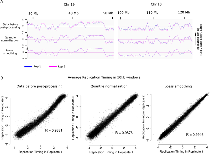
A.: Replication timing (RT) profiles of two technical repli-seq replicates (F121–9 mouse ESC, mapped on mm10) before and after each normalization step. Data are visualized using IGV. B.: Correlation between log ratio early / late at indicated step of normalization of 50kb windows along the genome of samples in A. R = Pearson correlation coefficient,

Accuracy

Repli-chip has successfully been used to assess RT in our lab^2,3,5–8, as part of the ENCODE consortium effort⁴⁹, and in other labs^50,51. We have shown that repli-seq gives similar results to repli-chip, in both human and mouse cells²⁵ (Figure 3), and that comparisons of genome-wide RT can be made between repli-seq and repli-chip. The two platforms can even be combined for clustering experiments²⁰. The advantages of repli-seq are the genomic coverage (including repetitive sequences), which is dependent only upon the mappability and sequencing depth, the ability to distinguish SNPs or parse phased genomes, and the ability to analyze any species with the same method.

Figure 3: Repli-chip and repli-seq give highly similar replication timing profiles at genome-wide level.

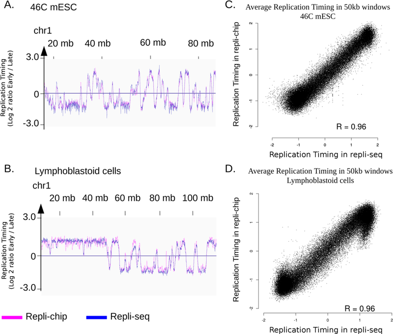
A. B.: Replication timing (RT) profile on a portion of chr1 of 46C mouse ESC (mm10) (A) and human lymphoblastoid cells (hg38) (B), visualized using IGV. RT is defined as the log2 ratio early fraction over late fraction (reads number is normalized on number of mapped reads for repli-seq). C. D.: correlation between average RT on 50kb windows on the whole genome in 46C mouse ESC (C) and human lymphoblastoid cells (D). Because repli-chip and repli-seq have different dynamic value ranges, data are scaled in R using the scale function, prior to visualisation. R = Pearson correlation coefficient.

Sequence specificity

The sequence information obtained from repli-seq can be used to discriminate between homologous regions. We here show an example using hybrid mouse embryonic stem cells (Figure 4) with a SNP density of ~1/100 bp. Discrimination of the maternal and paternal genomes reveals subtle differences between homologous regions. The capacity to discriminate two homologous chromosomes using our repli-seq procedure could be used to assess RT of the two X chromosomes in female cells, which replicate at different times during S phase (the active X replicates during early S phase, while the inactive X replicates during late S phase)^31,52,53. It is also useful to investigate the evolution of RT and the influence of DNA sequence variation vs. epigenetics (e.g. imprinting) on the regulation of RT^21,22. Finally, we anticipate repli-seq being invaluable for comparing genetically manipulated homologues to unmanipulated control homologues to investigate cis-acting elements regulating RT, and the applications of bar-coded lineage tracing⁵⁴ and high-throughput reporter assays²⁴ to the study of RT.

Figure 4: Repli-seq allows the discrimination between haplotypes.

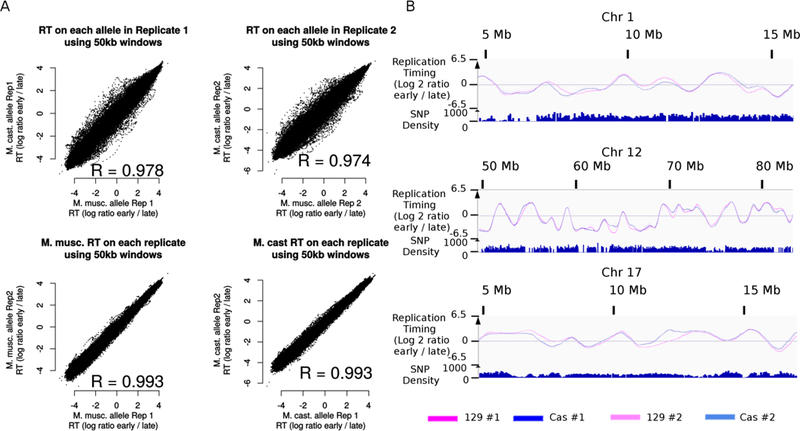
A.: Comparison of RT in F121–9 mouse hybrid ES cells (M. musculus / M. castaneus hybrid cells). The mapping on the two genomes has been performed as described in Supplementary Method V, then log ratio datasets have been quantile normalized and Loess smoothed. Replication timing in 50kb windows for each allele and each replicate has been plotted using R. B.: Comparison of RT for three homologous regions in the same cells. Data are visualized using IGV. R = Pearson correlation coefficient.

REFERENCES

- 1.Weber TS, Jaehnert I, Schichor C, Or-Guil M & Carneiro J Quantifying the Length and Variance of the Eukaryotic Cell Cycle Phases by a Stochastic Model and Dual Nucleoside Pulse Labelling. PLOS Comput. Biol 10, e1003616 (2014). [DOI] [PMC free article] [PubMed] [Google Scholar]
- 2.Hiratani I et al. Global Reorganization of Replication Domains During Embryonic Stem Cell Differentiation. PLOS Biol. 6, e245 (2008). [DOI] [PMC free article] [PubMed] [Google Scholar]
- 3.Hiratani I et al. Genome-wide dynamics of replication timing revealed by in vitro models of mouse embryogenesis. Genome Res. 20, 155–169 (2010). [DOI] [PMC free article] [PubMed] [Google Scholar]
- 4.Hansen RS et al. Sequencing newly replicated DNA reveals widespread plasticity in human replication timing. Proc. Natl. Acad. Sci 107, 139–144 (2010). [DOI] [PMC free article] [PubMed] [Google Scholar]
- 5.Pope BD, Hiratani I & Gilbert DM Domain-wide regulation of DNA replication timing during mammalian development. Chromosome Res. 18, 127–136 (2010). [DOI] [PMC free article] [PubMed] [Google Scholar]
- 6.Ryba T et al. Evolutionarily conserved replication timing profiles predict long-range chromatin interactions and distinguish closely related cell types. Genome Res. 20, 761–770 (2010). [DOI] [PMC free article] [PubMed] [Google Scholar]
- 7.Ryba T et al. Replication Timing: A Fingerprint for Cell Identity and Pluripotency. PLOS Comput. Biol 7, e1002225 (2011). [DOI] [PMC free article] [PubMed] [Google Scholar]
- 8.Rivera-Mulia JC et al. Dynamic changes in replication timing and gene expression during lineage specification of human pluripotent stem cells. Genome Res. 25, 1091–1103 (2015). [DOI] [PMC free article] [PubMed] [Google Scholar]
- 9.Sima J & Gilbert DM Complex correlations: Replication Timing and Mutational Landscapes during Cancer and Genome Evolution. Curr. Opin. Genet. Dev 25, 93–100 (2014). [DOI] [PMC free article] [PubMed] [Google Scholar]
- 10.Renard-Guillet C, Kanoh Y, Shirahige K & Masai H Temporal and spatial regulation of eukaryotic DNA replication: From regulated initiation to genome-scale timing program. Semin. Cell Dev. Biol 30, 110–120 (2014). [DOI] [PubMed] [Google Scholar]
- 11.Koren A DNA replication timing: Coordinating genome stability with genome regulation on the X chromosome and beyond. BioEssays 36, 997–1004 (2014). [DOI] [PubMed] [Google Scholar]
- 12.Sequeira-Mendes J & Gutierrez C Links between genome replication and chromatin landscapes. Plant J. 83, 38–51 (2015). [DOI] [PubMed] [Google Scholar]
- 13.Boulos RE, Drillon G, Argoul F, Arneodo A & Audit B Structural organization of human replication timing domains. FEBS Lett. 589, 2944–2957 (2015). [DOI] [PubMed] [Google Scholar]
- 14.Dileep V, Rivera-Mulia JC, Sima J & Gilbert DM Large-Scale Chromatin Structure-Function Relationships during the Cell Cycle and Development: Insights from Replication Timing. Cold Spring Harb. Symp. Quant. Biol 80, 53–63 (2015). [DOI] [PubMed] [Google Scholar]
- 15.Rivera-Mulia JC & Gilbert DM Replication timing and transcriptional control: beyond cause and effect — part III. Curr. Opin. Cell Biol 40, 168–178 (2016). [DOI] [PMC free article] [PubMed] [Google Scholar]
- 16.Gilbert DM Temporal order of replication of Xenopus laevis 5S ribosomal RNA genes in somatic cells. Proc. Natl. Acad. Sci. U. S. A 83, 2924–2928 (1986). [DOI] [PMC free article] [PubMed] [Google Scholar]
- 17.Gilbert DM & Cohen SN Bovine papilloma virus plasmids replicate randomly in mouse fibroblasts throughout S phase of the cell cycle. Cell 50, 59–68 (1987). [DOI] [PubMed] [Google Scholar]
- 18.Ryba T, Battaglia D, Pope BD, Hiratani I & Gilbert DM Genome-scale analysis of replication timing: from bench to bioinformatics. Nat. Protoc 6, 870–895 (2011). [DOI] [PMC free article] [PubMed] [Google Scholar]
- 19.Wilson KA, Elefanty AG, Stanley EG & Gilbert DM Spatio-temporal reorganization of replication foci accompanies replication domain consolidation during human pluripotent stem cell lineage specification. Cell Cycle 15, 2464–2475 (2016). [DOI] [PMC free article] [PubMed] [Google Scholar]
- 20.Sasaki T et al. Stability of patient-specific features of altered DNA replication timing in xenografts of primary human acute lymphoblastic leukemia. Exp. Hematol 51, 71–82.e3 (2017). [DOI] [PMC free article] [PubMed] [Google Scholar]
- 21.Koren A et al. Genetic Variation in Human DNA Replication Timing. Cell 159, 10151026 (2014). [DOI] [PMC free article] [PubMed] [Google Scholar]
- 22.Mukhopadhyay R et al. Allele-Specific Genome-wide Profiling in Human Primary Erythroblasts Reveal Replication Program Organization. PLOS Genet. 10, e1004319 (2014). [DOI] [PMC free article] [PubMed] [Google Scholar]
- 23.Bartholdy B, Mukhopadhyay R, Lajugie J, Aladjem MI & Bouhassira EE Allele-specific analysis of DNA replication origins in mammalian cells. Nat. Commun 6, (2015). [DOI] [PMC free article] [PubMed] [Google Scholar]
- 24.Akhtar W et al. Chromatin Position Effects Assayed by Thousands of Reporters Integrated in Parallel. Cell 154, 914–927 (2013). [DOI] [PubMed] [Google Scholar]
- 25.Pope BD et al. Topologically-associating domains are stable units of replication-timing regulation. Nature 515, 402–405 (2014). [DOI] [PMC free article] [PubMed] [Google Scholar]
- 26.Yue F et al. A comparative encyclopedia of DNA elements in the mouse genome. Nature 515, 355–364 (2014). [DOI] [PMC free article] [PubMed] [Google Scholar]
- 27.Dixon JR et al. Chromatin architecture reorganization during stem cell differentiation. Nature 518, 331–336 (2015). [DOI] [PMC free article] [PubMed] [Google Scholar]
- 28.Ryba T et al. Abnormal developmental control of replication-timing domains in pediatric acute lymphoblastic leukemia. Genome Res. 22, 1833–1844 (2012). [DOI] [PMC free article] [PubMed] [Google Scholar]
- 29.Hansen RS, Canfield TK, Lamb MM, Gartler SM & Laird CD Association of fragile X syndrome with delayed replication of the FMR1 gene. Cell 73, 1403–1409 (1993). [DOI] [PubMed] [Google Scholar]
- 30.Gilbert DM Evaluating genome-scale approaches to eukaryotic DNA replication. Nat. Rev. Genet 11, 673–684 (2010). [DOI] [PMC free article] [PubMed] [Google Scholar]
- 31.Koren A & McCarroll SA Random replication of the inactive X chromosome. Genome Res. 24, 64–69 (2014). [DOI] [PMC free article] [PubMed] [Google Scholar]
- 32.Dileep V, Didier R & Gilbert DM Genome-wide analysis of replication timing in mammalian cells: Troubleshooting problems encountered when comparing different cell types. Methods 57, 165–169 (2012). [DOI] [PMC free article] [PubMed] [Google Scholar]
- 33.Rivera-Mulia JC & Gilbert DM Replicating Large Genomes: Divide and Conquer. Mol. Cell 62, 756–765 (2016). [DOI] [PMC free article] [PubMed] [Google Scholar]
- 34.Cornacchia D et al. Mouse Rif1 is a key regulator of the replication-timing programme in mammalian cells. EMBO J. 31, 3678–3690 (2012). [DOI] [PMC free article] [PubMed] [Google Scholar]
- 35.Robinson JT et al. Integrative genomics viewer. Nat. Biotechnol 29, 24–26 (2011). [DOI] [PMC free article] [PubMed] [Google Scholar]
- 36.Nicol JW, Helt GA, Blanchard SG, Raja A & Loraine AE The Integrated Genome Browser: free software for distribution and exploration of genome-scale datasets. Bioinformatics 25, 2730–2731 (2009). [DOI] [PMC free article] [PubMed] [Google Scholar]
- 37.Kent WJ et al. The Human Genome Browser at UCSC. Genome Res. 12, 996–1006 (2002). [DOI] [PMC free article] [PubMed] [Google Scholar]
- 38.Weddington N et al. ReplicationDomain: a visualization tool and comparative database for genome-wide replication timing data. BMC Bioinformatics 9, 530 (2008). [DOI] [PMC free article] [PubMed] [Google Scholar]
- 39.Rasmussen TP et al. Messenger RNAs encoding mouse histone macroH2A1 isoforms are expressed at similar levels in male and female cells and result from alternative splicing. Nucleic Acids Res. 27, 3685–3689 (1999). [DOI] [PMC free article] [PubMed] [Google Scholar]
- 40.Development Core Team, R: A language and environment for statistical computing R Foundation for Statistical Computing, Vienna, Austria: ISBN 3-900051-07-0. (2005). [Google Scholar]
- 41.Bolstad BM, Irizarry RA, Åstrand M & Speed TP A comparison of normalization methods for high density oligonucleotide array data based on variance and bias. Bioinformatics 19, 185–193 (2003). [DOI] [PubMed] [Google Scholar]
- 42.Langmead B & Salzberg SL Fast gapped-read alignment with Bowtie 2. Nat. Methods 9, 357–359 (2012). [DOI] [PMC free article] [PubMed] [Google Scholar]
- 43.Li H et al. The Sequence Alignment/Map format and SAMtools. Bioinforma. Oxf. Engl 25, 2078–2079 (2009). [DOI] [PMC free article] [PubMed] [Google Scholar]
- 44.Quinlan AR & Hall IM BEDTools: a flexible suite of utilities for comparing genomic features. Bioinformatics 26, 841–842 (2010). [DOI] [PMC free article] [PubMed] [Google Scholar]
- 45.Lee PY, Costumbrado J, Hsu C-Y & Kim YH Agarose Gel Electrophoresis for the Separation of DNA Fragments. J. Vis. Exp. JoVE (2012). doi: 10.3791/3923 [DOI] [PMC free article] [PubMed] [Google Scholar]
- 46.Yokochi T et al. G9a selectively represses a class of late-replicating genes at the nuclear periphery. Proc. Natl. Acad. Sci. U. S. A 106, 19363–19368 (2009). [DOI] [PMC free article] [PubMed] [Google Scholar]
- 47.Takebayashi S et al. Murine esBAF chromatin remodeling complex subunits BAF250a and Brg1 are necessary to maintain and reprogram pluripotency-specific replication timing of select replication domains. Epigenetics Chromatin 6, 42 (2013). [DOI] [PMC free article] [PubMed] [Google Scholar]
- 48.Pope BD et al. DNA Replication Timing Is Maintained Genome-Wide in Primary Human Myoblasts Independent of D4Z4 Contraction in FSH Muscular Dystrophy. PLOS ONE 6, e27413 (2011). [DOI] [PMC free article] [PubMed] [Google Scholar]
- 49.Stamatoyannopoulos JA et al. An encyclopedia of mouse DNA elements (Mouse ENCODE). Genome Biol. 13, 418 (2012). [DOI] [PMC free article] [PubMed] [Google Scholar]
- 50.Fernandez-Vidal A et al. A role for DNA polymerase θ in the timing of DNA replication. Nat. Commun 5, 4285 (2014). [DOI] [PubMed] [Google Scholar]
- 51.Hadjadj D et al. Characterization of the replication timing program of 6 human model cell lines. Genomics Data 9, 113–117 (2016). [DOI] [PMC free article] [PubMed] [Google Scholar]
- 52.Morishima A, Grumbach MM & Taylor JH Asynchronous Duplication of Human Chromosomes and the Origin of Sex Chromatin. Proc. Natl. Acad. Sci 48, 756–763 (1962). [DOI] [PMC free article] [PubMed] [Google Scholar]
- 53.Takagi N, Sugawara O & Sasaki M Regional and temporal changes in the pattern of X-chromosome replication during the early post-implantation development of the female mouse. Chromosoma 85, 275–286 (1982). [DOI] [PubMed] [Google Scholar]
- 54.McKenna A et al. Whole-organism lineage tracing by combinatorial and cumulative genome editing. Science 353, aaf7907 (2016). [DOI] [PMC free article] [PubMed] [Google Scholar]
KEY REFERENCES:
- Ryba T, Battaglia D, Pope BD, Hiratani I & Gilbert DM Genome-scale analysis of replication timing: from bench to bioinformatics. Nat. Protoc 6, 870–895 (2011) [DOI] [PMC free article] [PubMed] [Google Scholar]
- Rivera-Mulia JC et al. Dynamic changes in replication timing and gene expression during lineage specification of human pluripotent stem cells. Genome Res. 25, 1091–1103 (2015). [DOI] [PMC free article] [PubMed] [Google Scholar]
- Wilson KA, Elefanty AG, Stanley EG & Gilbert DM Spatio-temporal re-organization of replication foci accompanies replication domain consolidation during human pluripotent stem cell lineage specification. Cell Cycle 15, 2464–2475 (2016). [DOI] [PMC free article] [PubMed] [Google Scholar]
Associated Data
This section collects any data citations, data availability statements, or supplementary materials included in this article.