Support Vector Machine Classification and Regression Prioritize Different Structural Features for Binary Compound Activity and Potency Value Prediction

Abstract

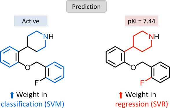
In computational chemistry and chemoinformatics, the support vector machine (SVM) algorithm is among the most widely used machine learning methods for the identification of new active compounds. In addition, support vector regression (SVR) has become a preferred approach for modeling nonlinear structure–activity relationships and predicting compound potency values. For the closely related SVM and SVR methods, fingerprints (i.e., bit string or feature set representations of chemical structure and properties) are generally preferred descriptors. Herein, we have compared SVM and SVR calculations for the same compound data sets to evaluate which features are responsible for predictions. On the basis of systematic feature weight analysis, rather surprising results were obtained. Fingerprint features were frequently identified that contributed differently to the corresponding SVM and SVR models. The overlap between feature sets determining the predictive performance of SVM and SVR was only very small. Furthermore, features were identified that had opposite effects on SVM and SVR predictions. Feature weight analysis in combination with feature mapping made it also possible to interpret individual predictions, thus balancing the black box character of SVM/SVR modeling.

1. Introduction

Supervised machine learning is a preferred approach for the prediction of compound properties including biological activity.^1,2 Among machine learning approaches, support vector machines (SVM) have become increasingly popular.³⁻⁵ The SVM methodology was originally conceived for binary class label prediction of objects⁶⁻⁸ on the basis of training data. In a given feature space, SVM learning aims to construct a hyperplane to best separate training data with different class labels.^7,8 The hyperplane is derived on the basis of a limited number of training instances, so-called support vectors, to maximize a margin on each side of the plane. If the data are not separable by a hyperplane, the data can be projected into feature spaces of higher dimensionality where linear separation of positive and negative examples might be possible.^7,8 For a given feature space, a successfully derived hyperplane represents a classification model that can then be used to predict the class label of test objects in this space, depending on which side of the hyperplane (i.e., the positive or negative) they fall. In chemoinformatics, binary class label prediction is used for compound classification, for example, to distinguish active from inactive compounds.^3,4 In addition to class label prediction, SVM models can also be used for compound database ranking by calculating their distance from the “active” or “inactive side” of the hyperplane.⁹

Support vector regression (SVR), an extension of the SVM algorithm, has been introduced for predicting numerical property values^10,11 such as compound potency. In SVR, instead of generating a hyperplane for class label prediction, a different function is derived on the basis of training data to predict numerical values. In analogy to SVM, SVR also projects training data with nonlinear structure–activity relationships (SARs) in a given feature space into higher-dimensional space representations where a linear regression function may be derived. In this case, compounds with different potency values are used to fit a regression model that can then be used to predict the potency of new candidate compounds. SVR typically produces statistically accurate regression models when predictions over all potency ranges are analyzed.^5,12 However, SVR also displays the tendency to underpredict highly potent compounds in data sets and hence eliminates activity cliffs from their activity landscape.¹²

In SVM and SVR, mapping into higher-dimensional feature spaces, which is a signature of these algorithms, is accomplished through the use of kernel functions, the so-called “kernel trick”.¹³ When using nonlinear kernel functions, SVM and SVR can resolve nonlinear SARs in original feature spaces through dimensionality extension. This makes SVR especially attractive for potency prediction because it is not confined to the applicability domain of conventional quantitative SAR analysis methods.¹⁴ On the other hand, both SVM and SVR modeling have black box character, meaning that the predictions cannot be directly interpreted in chemical terms. Hence, it is generally difficult to rationalize model performance. Only few attempts have thus far been made to aid in SVM model interpretation in high-dimensional kernel spaces. For example, support vectors with largest contributions to SVM models have been visualized.¹⁵ In addition, descriptor features have been organized in polar coordinate systems according to their contributions to SVM predictions.¹⁶

To increase model interpretability and reduce the black box character of SVM and SVR, we aimed to identify descriptor features that determine model performance on individual compound data sets. Given the close methodological relationship between SVM and SVR, relevant features of classification and regression models were also compared. Intuitively, one might expect that SVM and SVR would prioritize similar features for a given compound data set because most informative chemical features for predicting whether a compound is active or not might also be relevant for predicting the magnitude of activity. For this purpose, feature weighting and mapping techniques were systematically applied. Feature mapping helped to rationalize the performance of SVM and SVR models.

2. Results and Discussion

2.1. Global Performance of SVM and SVR Models

A prerequisite for feature weight analysis is the assessment of the prediction accuracy of SVM and SVR models. This is the case because the evaluation of features that contribute to predictions is only meaningful if the underlying models reach a reasonably high-performance level. Figure 1 summarizes the performance of our SVM and SVR models on the 15 activity classes using different figures of merit appropriate for assessing classification and regression calculations. Results are presented for two molecular representations, the MACCS fingerprint and extended connectivity fingerprint with bond diameter 4 (ECFP4). Figure 1a shows that the median F1 scores and the area under the ROC curve (AUC) values of the SVM models were clearly above 0.95 for both MACCS and ECFP4 fingerprints, reflecting accurate classification of active and inactive compounds. Furthermore, recall rates of the active compounds reached a median value of 0.77 for MACCS and 0.94 for ECFP4 among the top 1% of the ranked compounds. These results also reflected the usually observed higher performance of ECFP4 relative to MACCS.

Figure 1.

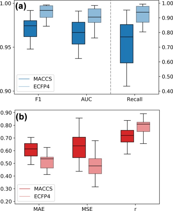
Global performance. Box plots report the prediction accuracy of (a) SVM and (b) SVR calculations over all activity classes and 10 independent trials per class. For SVM calculations, the F1 score, AUC, and recall of active compounds among the top 1% of the ranked test set are reported. For SVR calculations, the MAE and MSE values and the Pearson correlation coefficient (r) for the observed and predicted potency values are given.

Figure 1b reports the performance of the SVR models across the different activity classes. The median values of mean absolute error (MAE) and mean squared error (MSE) median values were between 0.5 and 0.6, and the median values of the Pearson correlation coefficient (r) between the predicted and observed pK_i values were above 0.7 for MACCS and above 0.8 for ECFP4. In addition, errors of potency predictions were consistently limited to less than 1 order of magnitude. Thus, the SVR model also exhibited an overall reasonable performance.

2.2. Feature Relevance

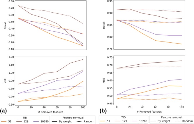
A second condition for informative feature weight analysis is demonstrating the relevance of individual fingerprint features. Therefore, features were randomly removed from SVM models or in the order of decreasing feature weights, and classification calculations were repeated. Figure 2 shows the results for exemplary activity classes and the MACCS (Figure 2a) and ECFP4 (Figure 2b) fingerprints. For MACCS containing 166 features, both random and weight-based feature removal decreased compound recall and increased MSE values. The magnitude of errors was greater for weight-based feature removal than for random feature removal. For ECFP4 comprising much larger numbers of possible features, random feature removal affected the calculations only marginally, if at all, whereas removal of highly weighted features led to a substantial reduction in compound recall and a gradual increase in MSE values. Thus, as anticipated, removal of features obtaining high weights during model building consistently reduced the model performance.

Figure 2.

Effects of feature removal. For SVM and SVR, the effects of iterative fingerprint feature removal on recall of active compounds and MSE are reported for three exemplary activity classes (with TID values according to Table 1) and the (a) MACCS and (b) ECFP4 fingerprints. Features were randomly removed (dashed lines) or in the order of decreasing feature weights (solid lines).

2.3. Global Feature Weight Analysis

For SVM and SVR models, weights of fingerprint features were systematically determined over 10 independent trials and compared. In some instances, feature weights were consistently high or low over different trials, as further detailed below; in others, they varied depending on the training data. In addition, feature weights generally varied for different activity classes, as expected. Furthermore, it was observed that some individual features were equally important for SVM and SVR for a given class, consistent with their shared methodological framework.

However, a striking finding was that the importance of many features for classification and regression fundamentally differed. Figures 3 and 4 show representative examples for different activity classes and MACCS and ECFP4, respectively. Feature weights were assigned to three different categories (i.e., high, medium, and low), as detailed in the Materials and Methods section. Figures 3a and 4a show examples of MACCS and ECFP4 features, respectively, which had very different weights in SVM and SVR models, including features with consistently—or mostly—low weights in classification and high weights in regression model and vice versa. Thus, many features were only relevant for either classification or regression. On average, 7 MACCS and 18 ECFP4 features were identified per activity class that had a high weight in at least 5 of the 10 SVM trials and a low weight in at least 5 SVR trials and vice versa. Among these, there were no MACCS and on an average one ECFP4 feature that exclusively had high/low weights in all SVM/SVR trials and vice versa. One possible explanation for such differences in feature relevance might be the composition of support vectors in SVM and SVR. Although SVM and SVR share a closely related methodological framework, support vectors for SVM and SVR are determined in different ways. To derive support vectors for regression, only active compounds are considered, whereas classification models are trained with active and inactive compounds, which also contribute to support vectors. Given these intrinsic differences, SVM and SVR models may prioritize different chemical descriptors for support vector compounds during the training stage.

Figure 3.

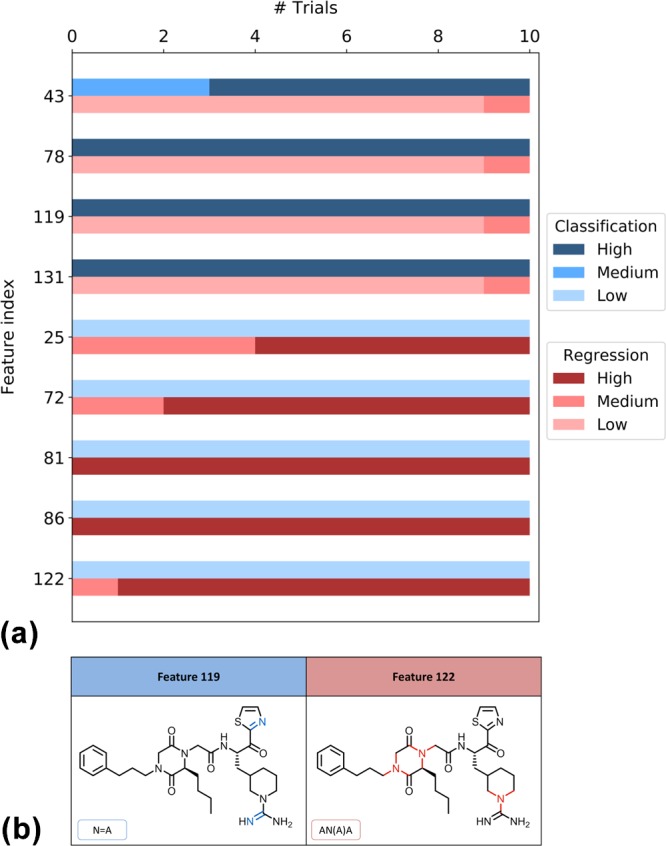
Distribution of MACCS feature weights and feature mapping. For an exemplary activity class (thrombin inhibitors, TID 11), (a) reports the distribution of weights of the selected features for SVM (classification, blue color) and SVR (regression, red color) over 10 trials. The color gradient represents the magnitude of feature weights (low, medium, or high). In (b), features that were highly weighted in SVM (blue color) and SVR (red color) are mapped on the same correctly predicted compound. In feature labels, “A” stands for any atom.

Figure 4.

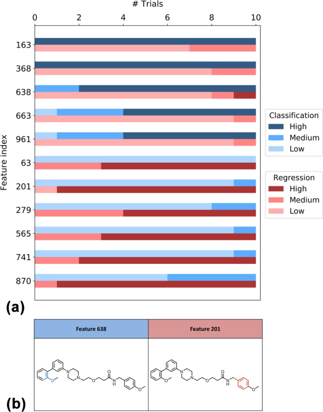
Distribution of ECFP4 feature weights and feature mapping. For an exemplary activity class (serotonin 1A (5-HT1A) receptor agonists, TID 51), (a) reports the distribution of weights of selected features for SVM (classification, blue color) and SVR (regression, red color) calculations over 10 trials. The color gradient represents the magnitude of feature weights (low, medium, or high). In (b), features that were highly weighted in SVM (blue color) and SVR (red color) are mapped on the same correctly predicted compound.

In Figures 3b and 4b, exemplary MACCS and ECFP4 features are mapped onto the structures of compounds that were correctly predicted. In Figure 3b, MACCS features that were highly weighted in classification (blue color) or regression (red color) were mapped onto the same molecule, a thrombin inhibitor, illustrating that features critical for SVM or SVR are often mapped to different parts of the same substructure. In Figure 4b, ECFP4 features critical for classification (blue color) or regression (red color) are mapped to a serotonin 1A (5-HT1A) receptor agonist, showing that features important for classification (feature 638) or regression (201) are mapped to distant parts of this compound.

In principle, features relevant for SVM and SVR might be activity class-specific or shared by different classes. To identify features common to different classes, MACCS and ECFP4 features were determined that had a high weight in at least 5 of the 10 SVM or SVR trials per class. For SVM, on an average, 9 of such MACCS and 15 ECFP4 features were identified per activity class and for SVR, 14 MACCS and 35 ECFP4 features were identified. For SVM, a total of 38 MACCS and 47 ECFP4 highly weighted features were shared by two activity classes. For SVR, 56 MACCS and 116 ECFP4 features were shared by two classes. However, for SVM (SVR), only five (seven) MACCS and nine (three) ECFP4 features with at least five high weights were common to five or more activity classes. Thus, most features determining SVM and SVR predictions were weighted in a compound class-specific manner.

Furthermore, we also determined the number of features that were consistently highly weighted in all trials per activity class. For SVM, on an average, only two of such MACCS and five ECFP4 features were identified and for SVR, two and four MACCS and ECFP4 features, respectively, were identified. Thus, weights of most features with strong contributions to SVM and SVR predictions displayed some variations in different activity classes depending on the training sets.

2.4. Features with Different Signs

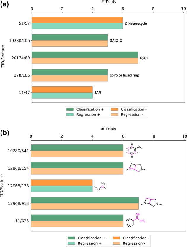
So far, only absolute feature weights were analyzed, which revealed many features that contributed differently to SVM and SVR. However, in SVM and SVR, feature weights may carry a positive or negative sign depending on how they influence the predictions. Features with a positive weight contribute to the prediction of active compounds in SVM and high potency values in SVR, whereas features with a negative weight contribute to the prediction of inactive compounds in classification and low potency values in regression. Thus, taking these signs into account further refines the view of differential feature contributions to SVM and SVR. Therefore, we also searched for features with high weights and different signs. Such features have opposite effects in SVM and SVR. Only few features were identified that had high weights in corresponding SVM and SVR trials but consistently different signs. Exemplary features with opposite effects in SVM and SVR are shown in Figure 5. For example, three MACCS features in Figure 5a contributed to the prediction of active compounds but low potency values (dark green/light orange bars) and two to the prediction of inactive compounds but high potency values of active compounds (light green/dark orange bars). In Figure 5b, four ECFP4 features are shown that contributed to the prediction of active compounds and low potency values and one that contributed to the prediction of inactive compounds and high potency values. Among features with high weights in both SVM and SVR, as discussed above, sign inversion and opposite effects in SVM and SVR were exceptions.

Figure 5.

Highly weighted features with different signs. For selected activity classes and (a) MACCS and (b) ECFP4 features (TID/feature), the number of trials is reported in which the features had high weights but different signs (+, −) in SVM and SVR. Features with positive weights contribute to the correct prediction of active compounds (dark green color) or high potency values (light green color), whereas features with negative weights contribute to the prediction of inactive compounds (dark orange bars) or low potency values (light orange bars). Bars are labeled with MACCS features (A, any atom and Q, heteroatom) or mapped ECFP4 atom environments (pink color).

2.5. Mapping of Highly Weighted Features

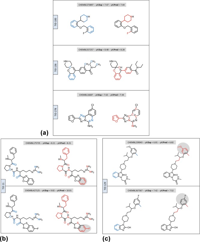
In Figure 6, highly weighted ECFP4 features are mapped on compounds from different activity classes that were correctly predicted using SVM and SVR. Atom environments were chosen for exemplary mapping because they have—by definition—a greater tendency to overlap than that involving discrete MACCS features. For an exemplary trial, features that had a high weight in the SVM and/or SVR model were mapped to the compounds shown. Figure 6a illustrates that only partly overlapping yet distinct atom environments led to the correct classification and potency value prediction of each compound.

Figure 6.

Mapping of highly weighted features. ECFP4 atom environments with high weights in classification and regression are mapped onto correctly classified compounds and potency prediction within 0.2 pK_i units. (a) shows individual compounds from three activity classes; (b,c) show pairs of analogues from two activity classes. Each compound is shown twice (side-by-side). On the left and right, features from classification (blue color) and regression (red color) are mapped, respectively. Single carbon atoms are displayed if they are a part of a mapped atom environment. In (b,c), substructures of analogues with feature differences are highlighted in gray color.

The two thrombin inhibitors in Figure 6b are close structural analogues that are only distinguished by a heteroatom replacement in a ring and a fluorine substituent. As anticipated for highly similar compounds, these inhibitors shared a number of features that were highly weighted in classification and regression models. However, two features highly weighted for regression but not classification were mapped to the ring substructure distinguishing these compounds. Clearly, in contrast to the SVM model that assigned the same highly weighted features to both inhibitors, in accordance with their common activity, the SVR model accounted for the structural difference between these compounds. Hence, feature mapping also indicated that the fluorine substitution might be responsible for the higher potency of the inhibitor at the bottom, given its positive weight.

The two mu-opioid receptor ligands in Figure 6c are also analogous to each other but distinguished from each other by multiple substitutions at the upper and lower ring. In this case, few highly weighted features were present, only one of which was shared by the classification and regression models, covering the methyl substituent at the upper phenyl ring. Other highly weighted features in the models were distinct and mapped to different substructures. In the SVR model, a highly weighted feature with negative contribution matched a part of the upper phenyl ring including the methoxy substituent of the compound at the top, indicating that this substructure (but not the lower ring) was important for potency variation among analogues.

Taken together, these examples illustrate that comparative mapping of features highly weighted in SVM and SVR helps to rationalize predictions made by classification and regression models and may reveal SAR information.

3. Conclusions

In this work, we have investigated and compared the relevance of different fingerprint features for the corresponding SVM and SVR models. The MACCS and ECFP4 fingerprints used herein capture the structural features of compounds in different ways. To these ends, feature weight analysis was carried out for well-performing classification and regression models over different compound classes. Because SVM and SVR share a common methodological framework, one might hypothesize that there should be considerable overlap between structural features that determine binary activity and potency value predictions. By contrast, systematic feature weight analysis revealed that features with high weights in SVM and SVR predominantly differed, a rather unexpected finding. In many instances, individual features contributed very differently to classification and regression, although features with strongly opposing effects were rare, as revealed by the analysis of positive and negative weights. SVM and SVR predictions are usually determined by feature combinations rather than individual features with high weights. Thus, features with medium weights also make contributions to predictions, albeit at a lesser magnitude than the most important ones. Therefore, as also demonstrated herein, mapping of highly weighted features is usually sufficient to identify molecular regions that are important for the activity-based classification and structural differences between compounds that are responsible for potency variation. Accordingly, mapping and comparing features that are highly weighted in SVM and SVR models help to better understand how individual features influence or determine predictions and thus alleviate the often-cited black box character of SVM, SVR, and other machine learning approaches that hinder model interpretation. Moreover, mapping of features that are highly weighted in SVR models onto compounds with correctly predicted potency values also points at SAR-informative regions in active compounds.

4. Materials and Methods

4.1. Compound Data Sets

Different sets of compounds with activity against human targets were extracted from ChEMBL version 22.¹⁷ Only compounds with numerically specified equilibrium constants (K_i values) for single human proteins with the highest assay confidence score were selected. If multiple K_i values for a compound and a target were available, they were averaged provided all values fell within the same order of magnitude; otherwise, the compound was discarded. Furthermore, compounds with a pK_i value below 5 were not selected to exclude borderline active compounds from modeling. In addition, this pK_i threshold also limited the range of potency values for SVR model building. Table 1 summarizes the 15 large activity classes that were selected. Each class contained at least 800 active compounds. In addition, for SVM modeling, 250 000 compounds were randomly selected from ZINC¹⁸ as a pool of negative (inactive) training and test instances. From this pool, negative training and test sets were randomly sampled for all classification calculations.

Table 1. Compound Data Sets^a.

TID	accession no.	target name	CPDs	median pKi	IQR pKi
11	P00734	thrombin	839	6.33	1.86
51	P08908	serotonin 1A (5-HT1A) receptor	1904	7.62	1.50
72	P14416	dopamine D2 receptor	2876	7.00	1.29
100	P23975	norepinephrine transporter	1099	6.82	1.60
129	P35372	mu-opioid receptor	2026	7.26	1.95
136	P41143	delta-opioid receptor	1547	7.11	1.97
137	P41145	kappa-opioid receptor	1930	7.28	2.07
138	P41146	nociceptin receptor	844	7.85	1.43
165	Q12809	HERG Homo sapiens	956	5.93	1.05
194	P00742	coagulation factor X	1476	8.05	2.80
278	P29275	adenosine A2b receptor	1187	7.23	1.43
10280	Q9Y5N1	histamine H3 receptor	2434	8.00	1.43
11362	P42336	PI3-kinase p110-α subunit	885	7.68	1.39
12968	O43614	orexin receptor 2	1040	6.70	1.57
20174	Q9Y5Y4	G protein-coupled receptor 44	833	7.65	1.90

^aComposition of 15 compound activity classes is reported that were selected for SVM and SVR modeling. For each class, the ChEMBL target ID (TID), accession number, target name, and number of compounds (CPDs) are given. In addition, median and interquartile range (IQR) pK_i values are reported, which were calculated from the pK_i distribution of each activity class.

4.2. Molecular Representation

Compounds were represented as MACCS¹⁹ and ECFP4 fingerprints.²⁰ MACCS is a prototypic binary-keyed fingerprint comprising 166 bits, each of which accounts for the presence or absence of a structural fragment or pattern. ECFP4 is a representative feature set fingerprint enumerating layered atom environments, which are encoded by integers using a hashing function. By design, ECFP4 has variable sizes, but it can be folded to obtain a fixed-length representation. For our calculations, ECFP4 was folded into a 1024-bit format using modulo mapping. Feature-to-bit mapping was recorded to enable mapping of fingerprint bits to compound structural features. Although modulo mapping assigns different features (atom environments) to identical bits, it is possible to trace environments and map them. Fingerprint representations were generated using in-house Python scripts based upon the OEChem toolkit.²¹

4.3. Support Vector Machine

For binary classification, training instances defined by a feature vector x ∈ X and a class label y ∈ {−1,1} are projected into the feature space X. For activity prediction, negative and positive examples represent inactive and active compounds for a given target, respectively. The SVM algorithm attempts to construct a hyperplane H such that the distance between the classes, the so-called margin, is maximized. This hyperplane is defined by a normal vector w and a scalar b using the expression H = {x|⟨w,x⟩ + b = 0}. For data that cannot be separated using a linear function, slack variables are added that permit training instances to fall within the margin or on the incorrect side of the hyperplane. To control the magnitude of allowed training errors, the cost or regularization hyperparameter C is introduced to balance margin size and classification errors. This represents a primal optimization problem that can be expressed in a dual form using Lagrange multipliers α_i (Lagrangian dual problem). Its solution yields the normal vector of the hyperplane w = ∑_iα_iy_ix_i. Training examples with nonzero coefficients represent the support vectors and correspond to data points of one class that are closest to the other, that is, those that lie on the margin of the hyperplane. Once the hyperplane is derived, test data are projected into the feature space and classified according to the side of the plane on which they fall, that is, f(x) = sgn(∑_iα_iy_i⟨x_i,x⟩ + b), or ranked using the real value, that is, g(x) = ∑_iα_iy_i⟨x_i,x⟩ + b.⁹

4.4. Support Vector Regression

Training samples for SVR are defined by a feature vector x ∈ X and a numerical label y ∈ R.^10,11 If SVR is applied to potency prediction, the numerical label is the pK_i value of the compound. SVR maps the training data as close as possible to the quantitative output y by deriving a regression function of the type f(x) = ⟨w,x⟩ + b. Tolerated deviations from the observed and predicted values of training data are at most ε, and larger errors are penalized. In SVR, the relaxation of error minimization problem is also controlled by a hyperparameter C, which penalizes large slack variables or deviations from the so-called ε tube. By solving the optimization problem with a Lagrange reformulation, the normal vector is derived and the prediction function is expressed as f(x) = ∑_iα_i⟨x_i,x⟩ + b.

4.5. Kernel Function

When accurate data separation is not feasible in the X space, the standard scalar product ⟨·,·⟩ is replaced by a kernel function K(·,·). Conceptually, the kernel function represents the scalar product in a high-dimensional space W in which the data might become linearly separable, without the need to compute an explicit mapping to W. This approach is known as the “kernel trick”¹³ that is applied in both SVM and SVR. In chemoinformatics, one of the most popular kernels for fingerprint representations is the Tanimoto kernel²² that was also used herein

4.6. Feature Weight Analysis

In the SVM model, different weights are assigned to molecular descriptors (features), which correspond to the coefficients of the primal optimization problem. The linear kernel (scalar product) allows direct determination of feature weights from the dual problem coefficients and support vectors. By contrast, direct access to feature weights is not possible when using nonlinear kernel functions because an explicit mapping into the high-dimensional feature space is not computed. However, for the Tanimoto kernel, feature weight analysis can be adapted from the linear case according to which the importance of a feature depends on the coefficients of those support vectors that contains the feature.¹⁶ To account for the nonlinearity of the Tanimoto formalism, a normalization factor is included for each individual support vector by dividing the feature weight contribution by the total number of features present in each support vector

Here, FW(d) is the feature weight for feature d, D is the dimensionality, m is the number of support vectors, and v_i and α_i are the support vector coefficients of the dual problem solution.

Feature contributions are not constant across feature space and depend on the fingerprint that is used.¹⁶ However, adaptation of feature weight analysis from the linear case with normalization yields an average weight, indicating the importance of each feature. Highly weighted fingerprint features can then be mapped to compound structures.¹⁶

4.7. Calculations and Data Analysis

Each activity class was randomly divided into training and test (prediction) sets comprising 700 and 100 compounds, respectively, following previously derived guidelines for relative training and test set composition.²³ For SVM, 700 and 100 compounds from ZINC database were randomly selected as negative training and test instances, respectively. For SVR, the same positive training data were used in each case (but no negative data). For each activity class and SVM/SVR calculation protocol, 10 independent trials were carried out, and the results were averaged.

For SVM and SVR models, the hyperparameter C was optimized using 10-fold cross-validation on training data using candidate values of 0.01, 0.1, 1, 5, 10, 20, 50, and 100. For SVM, hyperparameter optimization was guided by maximizing the F1 score; for SVR, optimization aimed to minimize the MAE.

Here, n is the number of samples (see also MSE given below).

Following hyperparameter optimization, feature weight analysis was carried out for classification and regression models. Weights were categorized as high, medium, or low, depending on whether their absolute value was at least 50, 25–50%, or less than 25% of the maximum weight observed for a given SVM model, respectively.

Binary activity (active/inactive) and potency values of test compounds were predicted, and model performance was estimated using different figures of merit. For SVM, the F1 score, AUC, and the recall of active compounds among the top 1% of the ranked test set were determined. For SVR, MAE, MSE, and the Pearson correlation coefficient between the observed and predicted pK_i values were calculated.

Calculation and data analysis protocols were implemented in Python using Scikit-learn.²⁴

Author Contributions

The study was carried out and the manuscript was written with contributions from all authors. All authors have approved the final version of the manuscript.

The authors declare no competing financial interest.

References

- Varnek A.; Baskin I. Machine Learning Methods for Property Prediction in Chemoinformatics: Quo Vadis?. J. Chem. Inf. Model. 2012, 52, 1413–1437. 10.1021/ci200409x. [DOI] [PubMed] [Google Scholar]
- Vogt M.; Bajorath J. Chemoinformatics: A View of the Field and Current Trends in Method Development. Bioorg. Med. Chem. 2012, 20, 5317–5323. 10.1016/j.bmc.2012.03.030. [DOI] [PubMed] [Google Scholar]
- Burbidge R.; Trotter M.; Buxton B.; Holden S. Drug Design by Machine Learning: Support Vector Machines for Pharmaceutical Data Analysis. Comput. Chem. 2001, 26, 5–14. 10.1016/s0097-8485(01)00094-8. [DOI] [PubMed] [Google Scholar]
- Geppert H.; Vogt M.; Bajorath J. Current Trends in Ligand-Based Virtual Screening: Molecular Representations, Data Mining Methods, New Application Areas, and Performance Evaluation. J. Chem. Inf. Model. 2010, 50, 205–216. 10.1021/ci900419k. [DOI] [PubMed] [Google Scholar]
- Heikamp K.; Bajorath J. Support Vector Machines for Drug Discovery. Expert Opin. Drug Discovery 2014, 9, 93–104. 10.1517/17460441.2014.866943. [DOI] [PubMed] [Google Scholar]
- Cortes C.; Vapnik V. Support-Vector Networks. Mach. Learn. 1995, 20, 273–297. 10.1007/bf00994018. [DOI] [Google Scholar]
- Burges C. J. C. A Tutorial on Support Vector Machines for Pattern Recognition. Data Min. Knowl. Discov. 1998, 2, 121–167. 10.1023/A:1009715923555. [DOI] [Google Scholar]
- Vapnik V. N.The Nature of Statistical Learning Theory, 2nd ed.; Springer: New York, 2000. [Google Scholar]
- Jorissen R. N.; Gilson M. K. Virtual Screening of Molecular Databases Using a Support Vector Machine. J. Chem. Inf. Model. 2005, 45, 549–561. 10.1021/ci049641u. [DOI] [PubMed] [Google Scholar]
- Drucker H.; Burges C. J. C.; Kaufman L.; Smola A.; Vapnik V. Support Vector Regression Machines. Adv. Neural Inform. Process. Syst 1997, 9, 155–161. [Google Scholar]
- Smola A. J.; Schölkopf B. A Tutorial on Support Vector Regression. Stat. Comput. 2004, 14, 199–222. 10.1023/b:stco.0000035301.49549.88. [DOI] [Google Scholar]
- Balfer J.; Bajorath J. Systematic Artifacts in Support Vector Regression-Based Compound Potency Prediction Revealed by Statistical and Activity Landscape Analysis. PLoS One 2015, 10, e0119301 10.1371/journal.pone.0119301. [DOI] [PMC free article] [PubMed] [Google Scholar]
- Boser B. E.; Guyon I. M.; Vapnik V. N.. A Training Algorithm for Optimal Margin Classifiers. In Proceedings of the Fifth Annual ACM Workshop on Computational Learning Theory; Pittsburgh, Pennsylvania, 1992; ACM: New York, 1992; pp 144–152. [Google Scholar]
- Cherkasov A.; Muratov E. N.; Fourches D.; Varnek A.; Baskin I. I.; Cronin M.; Dearden J.; Gramatica P.; Martin Y. C.; Todeschini R.; Consonni V.; Kuz’min V. E.; Cramer R.; Benigni R.; Yang C.; Rathman J.; Terfloth L.; Gasteiger J.; Richard A.; Tropsha A. QSAR Modeling: Where Have You Been? Where Are You Going To?. J. Med. Chem. 2014, 57, 4977–5010. 10.1021/jm4004285. [DOI] [PMC free article] [PubMed] [Google Scholar]
- Hansen K.; Baehrens D.; Schroeter T.; Rupp M.; Müller K.-R. Visual Interpretation of Kernel-Based Prediction Models. Mol. Inf. 2011, 30, 817–826. 10.1002/minf.201100059. [DOI] [PubMed] [Google Scholar]
- Balfer J.; Bajorath J. Visualization and Interpretation of Support Vector Machine Activity Predictions. J. Chem. Inf. Model. 2015, 55, 1136–1147. 10.1021/acs.jcim.5b00175. [DOI] [PubMed] [Google Scholar]
- Gaulton A.; Bellis L. J.; Bento A. P.; Chambers J.; Davies M.; Hersey A.; Light Y.; McGlinchey S.; Michalovich D.; Al-Lazikani B.; Overington J. P. ChEMBL: a large-scale bioactivity database for drug discovery. Nucleic Acids Res. 2012, 40, D1100–D1107. 10.1093/nar/gkr777. [DOI] [PMC free article] [PubMed] [Google Scholar]
- Irwin J. J.; Sterling T.; Mysinger M. M.; Bolstad E. S.; Coleman R. G. ZINC: A Free Tool to Discover Chemistry for Biology. J. Chem. Inf. Model. 2012, 52, 1757–1768. 10.1021/ci3001277. [DOI] [PMC free article] [PubMed] [Google Scholar]
- MACCS Structural Keys; Accelrys: San Diego, CA, 2011.
- Rogers D.; Hahn M. Extended-Connectivity Fingerprints. J. Chem. Inf. Model. 2010, 50, 742–754. 10.1021/ci100050t. [DOI] [PubMed] [Google Scholar]
- OEChem TK, version 2.0.0; OpenEye Scientific Software: Santa Fe, NM, 2015.
- Ralaivola L.; Swamidass S. J.; Saigo H.; Baldi P. Graph Kernels for Chemical Informatics. Neural Network. 2005, 18, 1093–1110. 10.1016/j.neunet.2005.07.009. [DOI] [PubMed] [Google Scholar]
- Rodríguez-Pérez R.; Vogt M.; Bajorath J. Influence of Varying Training Set Composition and Size on Support Vector Machine-Based Prediction of Active Compounds. J. Chem. Inf. Model. 2017, 57, 710–716. 10.1021/acs.jcim.7b00088. [DOI] [PMC free article] [PubMed] [Google Scholar]
- Pedregosa F.; Varoquaux G.; Gramfort A.; Michel V.; Thirion B.; Grisel O.; Blondel M.; Prettenhofer P.; Weiss R.; Dubourg V.; Vanderplas J.; Passos A.; Cournapeau D.; Brucher M.; Perrot M.; Duchesnay E. Scikit-learn: Machine Learning in Python. J. Mach. Learn. Res. 2011, 12, 2825–2830. [Google Scholar]