Using thresholds in noise to identify hidden hearing loss in humans

Abstract

Objectives

Recent animal studies suggest that noise-induced synaptopathy may underlie a phenomenon that has been labeled hidden hearing loss (HHL). Noise exposure preferentially damages low spontaneous-rate auditory-nerve fibers, which are involved in the processing of moderate-to-high level sounds and are more resistant to masking by background noise. Therefore, the effect of synaptopathy may be more evident in suprathreshold measures of auditory function, especially in the presence of background noise. The purpose of this study was to develop a statistical model for estimating HHL in humans using thresholds in noise as the outcome variable and measures that reflect the integrity of sites along the auditory pathway as explanatory variables. Our working hypothesis is that HHL is evident in the portion of the variance observed in thresholds in noise that is not dependent on thresholds in quiet, because this residual variance retains statistical dependence on other measures of suprathreshold function.

Design

Study participants included 13 adults with normal hearing (≤15 dB HL) and 20 adults with normal hearing at 1 kHz and sensorineural hearing loss at 4 kHz (>15 dB HL). Thresholds in noise were measured and the residual of the correlation between thresholds in noise and thresholds in quiet, which we refer to as thresholds-in-noise residual, was used as the outcome measure for the model. Explanatory measures were (1) auditory brainstem response (ABR) Waves I and V amplitudes, (2) electrocochleographic action potential (AP) and summating potential (SP) amplitudes, (3) distortion-product otoacoustic emissions (DPOAE) level, and (4) categorical loudness scaling (CLS). All measurements were made at two frequencies (1 and 4 kHz). ABR and ECochG measurements were made at 80 and 100 dB peSPL, while wider ranges of levels were tested during DPOAE and CLS measurements. A model relating the thresholds-in-noise residual and the explanatory measures was created using multiple linear regression analysis.

Results

Predictions of thresholds-in-noise residual using the model accounted for 61% (p<0.01) and 48% (p<0.01) of the variance in the measured thresholds-in-noise residual at 1 and 4 kHz, respectively.

Conclusions

Measures of thresholds in noise, SP/AP ratio, and ABR Waves I and V amplitude may be useful for the prediction of HHL in humans. With further development, our approach of quantifying HHL by the variance that remains in suprathreshold measures of auditory function after removing the variance due to thresholds in quiet, together with our statistical modeling, may provide a quantifiable and verifiable estimate of HHL in humans with normal hearing and with hearing loss. The current results are consistent with the view that inner hair cell and auditory-nerve pathology may underlie suprathreshold auditory performance.

INTRODUCTION

Sensorineural hearing loss (SNHL) may occur as a result of dysfunction of outer hair cells (OHC), inner hair cells (IHC), auditory-nerve fibers (ANF), or synapses. Whereas OHC dysfunction is accompanied by elevated audiometric thresholds, making it evident in clinical evaluations, IHC, ANF and synaptic dysfunctions are more difficult to detect. SNHL that does not elevate thresholds in quiet, and therefore is not identified by standard clinical techniques, has been referred to as “hidden hearing loss” (HHL). Evidence from studies with laboratory animals suggests that noise-induced synaptic dysfunction (i.e., synaptopathy), may explain HHL (Kujawa & Liberman 2009; Lin et al. 2011; Furman et al. 2013; Mehraei et al. 2016). The data from these studies showed that noise exposure preferentially damaged low and medium spontaneous-rate (SR) ANFs (sometimes collectively referred to as low-SR ANFs), which are involved in the processing of moderate-to-high level sounds and are more resistant to masking by background noise. Therefore, the effect of synaptopathy may be more evident in suprathreshold measures of auditory function, especially in the presence of background noise. Understanding HHL in humans requires the use of measurements that reveal the functional integrity of sites along the auditory pathway (OHCs, IHCs, ANFs, synapses) in combination with measurements that are sensitive to the group of ANFs (low vs. high SR) underlying the dysfunction. Thresholds in noise may be sensitive to loss of low-SR fibers. The purpose of this study was to establish a theoretical framework for the development of a statistical model for estimating HHL in humans using thresholds in noise as the outcome variable and several auditory measures that reflect the integrity of sites along the auditory pathway as explanatory variables. Thresholds-in-noise residual may provide a functional and quantitative proxy for HHL because it represents the portion of the variance in thresholds in noise that is not dependent on thresholds in quiet, but is evident in other measures of suprathreshold function.

One possible cause of HHL is cochlear synaptopathy, which has been associated with exposure to high-level noise (e.g. Kujawa & Liberman 2009). In several studies with laboratory animals, noise exposure resulting in temporary threshold shift led to irreversible cochlear synaptopathy even when there was no hair-cell loss and both audiometric thresholds and otoacoustic emissions returned to normal (e.g. Kujawa & Liberman 2009; Furman et al. 2013; Liberman & Liberman 2015). This synaptopathy was usually followed by neuropathy, i.e. neural degeneration. Synaptopathy due to noise exposure was more prevalent in low-SR and medium-SR (sometimes collectively referred to as low-SR), high-threshold ANFs compared to high-SR, low-threshold ANFs (Furman et al. 2013; Liberman & Liberman 2015). Audiometry may be insensitive to synaptopathy because threshold responses primarily involve high-SR ANFs. Additionally, audiometry is a signal-detection task that may not require the full complement of ANFs. The coding of suprathreshold sound features, on the other hand, may involve low-SR fibers (Liberman 1978; Costalupes et al. 1984; Bharadwaj et al. 2014). These fibers are also more resistant to masking by background noise (Costalupes 1985; Young & Barta 1986). Changes to suprathreshold measures, such as auditory brainstem response (ABR) Wave-V latencies with noise level (Mehraei et al. 2016) and middle-ear muscle reflexes (Valero et al. 2016) have been observed following noise-induced cochlear synaptopathy, while temporal coding abilities vary with noise history (Ruggles et al. 2011; Bharadwaj et al. 2015). Because synaptopathy affects low-SR fibers, it may be the cause of suprathreshold processing difficulties in humans (e.g. Kujawa & Liberman 2009; Furman et al. 2013; Plack et al. 2014; Mehraei et al. 2016; Liberman et al. 2016). There is, however, scant evidence that the observations made in animal studies also apply in humans, due mainly to the inapplicability of the invasive measurement techniques that were used in animal studies to diagnose synaptopathy. Furthermore, a definition of HHL that can be applied in humans, is quantifiable, and is capable of being validated remains elusive. Translation to humans requires a definition of HHL that distinguishes it from threshold elevation (e.g. Hickox et al. 2017; Le Prell and Clavier, 2016). To be clinically relevant, this definition must be based on noninvasive measurements that are both specific to the site of lesion (OHC, IHC, ANF and/or synapses) and to the spontaneous-rate class of the auditory fibers (low SR vs. high SR) underlying the dysfunction.

Thresholds in noise may be sensitive to cochlear synaptopathy. Lobarinas et al. (2016) showed that selective carboplatin-induced IHC loss in chinchillas led to elevated thresholds in noise, while thresholds in quiet remained unchanged. Currently, functional tests of IHC loss in humans do not exist. However, the amplitude of ABR Wave I may be sensitive to IHC deafferentation (Kujawa & Liberman 2009; Wynne et al. 2013). Studies with laboratory animals treated with carboplatin to induce IHC loss, without OHC loss, demonstrated reductions in the amplitude of ABR Wave I (Wang et al. 2002; El-Badry & McFadden 2007) that were similar to Wave I amplitude reductions caused by the noise-induced cochlear synaptopathy. In addition, synchronization of ANF discharges to a sound’s waveform decreases in noise backgrounds (Henry and Heinz, 2012). Therefore, a portion of the variance in measurements of thresholds in noise may be a consequence of damage to IHCs and ANFs in some, but not all, cases. We hypothesized that performance on the thresholds-in-noise task would reflect the degree of HHL.

The present study describes a framework for the development of a multiple linear regression (MLR) model of HHL. In the model, thresholds in noise, a suprathreshold measure that is presumably influenced by HHL, served as the outcome variable. Our hypothesis was that the variance in thresholds in noise is partly dependent on the integrity of ANFs. We take the approach of using a MLR model to estimate HHL because direct observation of cochlear synaptopathy is not possible in vivo in humans. Synaptopathy has been observed, though, in cadaveric preparations of human temporal bones, in which quantification of synapses were related to age (Viana et al., 2015). Several measures that reflect the functional integrity of sites along the auditory pathway served as explanatory variables. These included ABR, electrocochleography (ECochG), distortion-product otoacoustic emissions (DPOAE), and categorical loudness scaling (CLS).

The amplitude of ABR Wave I (which is also referred to as the action potential (AP) in ECochG literature) has been used as an indirect measure of cochlear synaptic health. Specifically, ABR Wave-I amplitude scaled with synaptic loss in animal studies (Kujawa & Liberman 2009; Lin et al. 2011; Furman et al. 2013; Mehraei et al. 2016; Liberman and Kujawa 2017) and with noise-exposure history in humans (Stamper & Johnson 2015a; Bramhall et al. 2017). Although a follow-up analysis to the Stamper and Johnson study showed that the relationship only held for females and not for males (Stamper & Johnson 2015b), these findings suggest that Wave I may be an indicator of cochlear synaptopathy. However, these relationships in humans are tenuous at best, perhaps in part because of issues with the reliability of reported noise-exposure histories, the variance in Wave I measurements and the lack of an accepted definition of HHL that can be quantified and validated. The detection of Wave V is related to audiometric thresholds and thus is used in the clinic to predict auditory status (e.g., Gorga et al. 2006; McCreery et al. 2015). The summating potential (SP), which includes contributions of both IHCs and OHCs (Durrant et al. 1998), serves as a proxy for hair-cell integrity. DPOAE level depends on cochlear amplification and OHC motility (e.g. Brownell 1990), and has been used as an indicator of OHC integrity (e.g., Lonsbury-Martin & Martin 1990; Gorga et al. 1997; Abdala & Visser-Dumont 2001). The health of OHCs is reflected in measurements of CLS, a measure of an individual’s loudness percept and loudness growth. CLS functions, which relate loudness in categorical units (CU) to sound pressure level (SPL), are characterized by two segments. The low-level segment relates to audiometric threshold (Al-Salim et al. 2010; Rasetshwane et al. 2015) and to DPOAE level (Thorson et al. 2012; Rasetshwane et al. 2013), and presumably, like DPOAEs, reflects OHC integrity. The high-level segment does not relate to either audiometric threshold (Al-Salim et al. 2010) or DPOAEs. In addition to OHCs, IHCs and central processes mediate loudness (e.g., Moore et al. 2004). We hypothesize that the high-level segment of the CLS is influenced by IHC and ANF function, and thus reflects the combined integrity of these auditory sites. As a result, the two segments of the CLS function may provide differential insight into OHC and more central auditory function.

Because noise exposure has been linked to synaptopathy in laboratory animals and synaptopathy has been suggested as a possible cause of suprathreshold deficits in humans, independent of other factors such as aging, quantification of an individual’s overall noise-exposure history is relevant to the assessment of HHL. A noise-exposure questionnaire (NEQ) has been used to assess noise-exposure history (Megerson 2010; Stamper & Johnson 2015a; Johnson et al. 2017). Stamper & Johnson (2015a) showed that noise-exposure history, as captured by the NEQ, was correlated with ABR Wave-I amplitude. However, a follow-up analysis showed that the relationship only held for females (Stamper & Johnson 2015b). Bramhall et al. (2017) also observed a relationship between noise-exposure history and Wave-I amplitude, using a questionnaire that is different from the NEQ. However, several studies (e.g. Prendergast et al. 2017; Spankovich et al 2017; Yeend et al. 2017) did not observe a relationship between noise-exposure history and Wave-I amplitude, as well as other measures that are presumably influenced by HHL. We will revisit this issue in the Discussion section.

Our approach for differential diagnosis of SNHL is similar to that of Lopez-Poveda and colleagues (Lopez-Poveda et al. 2009; Lopez-Poveda & Johannesen 2012; Johannesen et al. 2014), Moore and colleagues (Moore & Glasberg 1997; Chen et al. 2011) and others (Jepsen & Dau 2011). These studies assumed that total SNHL was the decibel (dB) sum of OHC loss and IHC loss. However, neural and synaptic dysfunctions also contribute to hearing difficulties, especially for suprathreshold sound and in the presence of competing masking sounds. We extend these earlier studies by including measures that reflect ANF function, and by removing the influence of threshold in quiet and then examining the relations between explanatory measures and the portion of the variance in thresholds in noise that cannot be attributed to peripheral factors.

Our efforts to develop methods to identify HHL in humans using correlational analysis and behavioral and physiological measures of auditory function follow several earlier studies (e.g. Ruggles et al. 2011; Bharadwaj et al. 2015; Mehraei et al. 2016; Liberman et al. 2016). Ruggles et al. (2011) observed correlations between the frequency-following response (an electrophysiological measure of sustained neural temporal coding) and spatial selective auditory attention (a behavioral measure that relies on interaural timing differences). In the same study, frequency-modulation detection, which also relies on temporal coding, was correlated with spatial selective auditory attention. Mehraei et al. (2016) showed that changes in ABR Wave-V latency with noise level were correlated with Wave-I amplitude growth. Individuals with presumed cochlear synaptopathy (based on measurements of temporal coding and results of similar ABR measurements in mice) had smaller Wave-V latency shifts in noise, which Mehraei et al. associated with loss of low-SR ANFs. Bharadwaj et al. (2015) demonstrated that poor performance on tasks evaluating selective attention and interaural time difference processing were weakly correlated with speech-in-noise perceptual deficit, which they associated with cochlear neuropathy as a result of noise exposure. Liberman et al. (2016) recently showed that normalizing the SP by dividing it by the AP (the SP/AP ratio) provides a better separation between groups of college students at low risk and high risk based on noise-exposure history, when compared to using the AP amplitude alone. This suggests that the SP/AP ratio, which has previously been suggested as having diagnostic value in Ménière’s disease (Levine et al. 1998; Ferraro & Durrant 2006), may also be useful in inferring synaptopathy.

In summary, we derive a statistical model that describes the relationship between thresholds in noise and ABR Waves I and V, SP, AP, SP/AP ratio, DPOAE and CLS. We assumed that (1) SP reflects both OHC and IHC integrity, (2) ABR Wave-I (AP) amplitude reflects ANF integrity, (3) SP/AP ratio reflects the integrity of hair cells relative to the integrity of ANFs, (4) DPOAE reflects OHC integrity, (5) ABR Wave-V amplitude reflects the health of the auditory system up to the brainstem, and (6) CLS reflects both OHC and IHC integrity. Here, we define integrity functionally, not in relation to the number of surviving hair cells or synaptic ribbons because histological analysis to determine the extent of anatomical loss is not possible in vivo in humans.

MATERIALS AND METHODS

Participants

A total of 33 adults participated in the present study. There were 20 participants (10 females) with sensorineural hearing loss (SNHL; mean age = 49.4, standard deviation (SD) = 7.0, range = 35–64 years) and 13 participants (7 females) with normal hearing (NH; mean age = 31.0, SD = 8.5, range = 23–48 years). All participants were assessed using standard audiometric procedures. Pure-tone air-conduction thresholds were measured at octave frequencies (0.25 to 8 kHz) and two inter-octave frequencies (3 and 6 kHz) (GSI 61, Grason-Stadler, Eden Prairie, Minnesota). Additionally, pure-tone bone-conduction thresholds were measured at octave frequencies from 0.25 to 4 kHz. Thresholds were measured in 2-dB steps at 1 and 4 kHz and 5-dB steps at all other frequencies. Participants with thresholds ≤ 15 dB hearing level (HL) at all frequencies were considered to have NH. Participants with thresholds >15 dB at 4 kHz were considered to have SNHL. Thresholds did not exceed 66 dB HL in any participant. All participants were required to have thresholds ≤ 15 dB at 1 kHz. Participants whose thresholds did not fall within the criteria for both 1 and 4 kHz were not included in the study. Participants were also excluded from the study if the air-bone gap was > 10 dB at any frequency. In addition to comparisons of air- and bone-conduction thresholds, 226-Hz tympanometry was used to assess middle-ear function (Madsen Otoflex 100, GN Otometrics, Denmark). Participants were included if middle-ear pressure ranged from +50 to −100 daPa and static compliance was between 0.3 and 2.5 cm³. Individuals with SNHL who had a family history of hearing loss, and/or history of ototoxic-drug exposure were excluded from the study.

All measurements were made monaurally. If both ears met the inclusion criteria for participants with NH, the ear with better audiometric thresholds was selected for testing. If both ears had similar audiometric thresholds, the test ear was selected randomly. If both ears met the inclusion criteria for participants with SNHL, the ear with audiometric thresholds in the mild-to-moderate range at 4 kHz was tested to increase the likelihood of responses above the noise floor for explanatory measurements. If both ears had thresholds in this range, the test ear was selected randomly. In all, data were collected from nine left and 11 right ears of participants with SNHL, and seven left and six right ears of participants with NH. In no case were both ears of the same subject included in the analyses.

Procedures

All procedures were approved by the Boys Town National Research Hospital (BTNRH) Institutional Review Board and informed consent was obtained from all participants.

Thresholds in noise

Thresholds in noise were measured using the threshold-equalizing noise (TEN) test (Moore et al. 2004). The TEN (HL) test was selected because simple procedures exist for the test, and the test has been used in several previous studies (e.g. Thabet 2009; Vinay et al. 2017). The passband of the TEN masker extends from about 0.4 to 7 kHz (see Moore et al. 2004 for more details). Measurements were performed monaurally on all subjects at 1 and 4 kHz using TDH-50P supra-aural headphones (Telephonics, Farmingdale, NY). Stimulus presentation for the TEN (HL) test was controlled using an audiometer (GSI 61, Grason-Stadler, Eden Prairie, Minnesota). The stimuli were generated on a computer, and routed to the audiometer through a 24-bit soundcard (Hammerfall DSP Multi-Face II, RME, Germany). Prior to the collection of data at 1 and 4 kHz, a practice trial was completed at 0.5 kHz. The level of the (TEN) masker was set to 70 dB HL for both frequencies, since all participants had thresholds less than 70 dB HL. The level of the tonal signal was adjusted in 2 dB steps to determine thresholds (Moore et al. 2004). The SNR, i.e. level of tone at threshold of detection minus the level of the TEN masker (70 dB HL) was calculated. Correlation analysis was then used to calculate the residual of the correlation of the SNR with thresholds in quiet. The residual SNR served as a proxy for HHL and was used as the outcome variable in the MLR model. This approach was based on the view that, by definition, the portion of the variance not accounted for by thresholds in quiet represented HHL. To our knowledge, this represents the first effort to quantitatively define HHL, which is necessitated because there is no gold standard for HHL. In the TEN test, SNR>10 dB is thought of as indicative of the presence of cochlear dead regions (Moore et al. 2004).

Electrophysiological Measurements

ABR and ECochG were measured simultaneously using custom-designed software (Cochlear Response (CResp) version 1.0, BTNRH, Omaha, NE) running on a computer equipped with a 24-bit soundcard (Babyface, RME, Haimhausen, Germany). Single-channel electroencephalographic (EEG) responses were acquired using surface electrodes placed at the high forehead (Fpz, ground) and the vertex (Cz, noninverting active), and in the ear canal using a tiptrode (inverting reference). Electrode impedances were ≤ 3 kΩ in all cases. During each recording, EEG activity was amplified (gain = 100 000) and filtered (0.1–1.5 kHz passband) (Opti-Amp 8001, Intelligent Hearing Systems, Miami, FL). After amplification and filtering, the signal was directed from the Opti-Amp transmitter, via a soundcard, to the computer for averaging. The soundcard utilized a sampling rate of 48 kHz. Stimuli were tonebursts at 1 and 4 kHz presented at a rate of 27/s. For both frequencies, the duration of the tone-burst was 1 ms. This stimulus duration resulted in large AP amplitudes during pilot testing. The tonebursts were presented at 80 and 100 dB peak-equivalent (pe) SPL using positive polarity at the onset of the stimulus. The stimuli were windowed using a Blackman function, which has equal rise and fall times with no plateau. The stimuli were routed to an ER-3A insert earphone (Etymōtic Research, Elk Grove Village, IL) connected to the soundcard. During the recording, responses were stored in two buffers with even-numbered responses being stored in one buffer and odd-numbered responses being stored in the other. This produced a simultaneous replication that served as a test of the reliability of the measurement within a measurement session. The sum of the two buffers was used to estimate the response and the difference between the buffers served as an estimate of the noise. Artifact rejection was utilized based on the peak absolute differences between buffers in order to discard any responses that were contaminated by transient noise. Responses that were accepted were synchronously averaged in separate buffers and displayed in the computer screen, to allow for monitoring during data collection. Data collection continued until a total of 4000 artifact-free responses (2000 per buffer) were collected. Two sets of measurements were collected, resulting in a total of four waveforms per participant at each frequency. The four waveforms were averaged to further improve the SNR.

Two examiners independently identified peaks and troughs of ABR Waves I and V and determined their latency and amplitude. Amplitude was calculated as the difference between the positive peak and the following trough of the waveform, while latency was calculated as the delay between the peak of the waveform and the stimulus onset. Amplitudes and latencies were determined to precisions of 0.02μV and 0.02 ms, respectively. When there was a disagreement between the two examiners, defined as a latency mismatch > 0.04 ms, a third examiner with extensive experience scoring ABRs evaluated the waveforms and selected the latency and amplitude. Latency only served as a guide in the identification of peaks and was not used in the statistical analysis. The mean of the amplitude obtained by the two examiners were used in subsequent analysis, unless there was a disagreement between the two examiners. Disagreements occurred in 13 of 516 possible conditions. It was always easier to identify wave V than wave I. However, there were instances when there was ambiguity in the identification of wave V, especially its trough. When this occurred, the most ambiguous of the four waveforms was excluded and the mean was calculated based on the remaining three waveforms.

Waveforms containing an identifiable SP were evaluated by two examiners (see Table 1 for number of participants contributing data for each explanatory variable). Because of the difficulty in identifying the presence of the SP, the two examiners worked together to identify the baseline, SP and AP in the ECochG waveforms. Baseline was selected as the midpoint of the alternating current signal resulting from either stimulus artifact or cochlear microphonic (Chertoff et al. 2012). If stimulus artifact was not present in the recording, the baseline was selected as the trough before or after the AP, whichever was clearer.

Table 1.

Explanatory variables that were measured separately at 1 and 4 kHz and number of participants contributing data to each variable. The stimulus level (in dB peSPL), where applicable, is indicated using subscript.

Variable	1 kHz	4 kHz
DPOAE level	31	31
L10 CU	32	32
L40 CU	32	32
Wave I80	16	27
Wave I100	31	31
Wave I difference	16	27
Wave V80	32	31
Wave V100	31	31
Wave V/Wave I ratio80	16	27
Wave V/Wave I ratio100	31	31
SP/AP ratio80	6	18
SP/AP ratio100	18	25
SP80	6	18
SP100	18	25
AP80	9	24
AP100	28	29
AP difference	8	23

For the MLR model, explanatory variables derived from ABR included Wave-I amplitude, Wave-V amplitude, Wave V-to-Wave I amplitude ratio and Wave I amplitude difference, i.e. Wave I amplitude at 100 dB peSPL minus Wave I amplitude at 80 dB peSPL. The SP, AP and the SP/AP ratio served as explanatory variables derived from ECochG. AP amplitude difference, i.e. AP amplitude at 100 dB peSPL minus AP amplitude at 80 dB peSPL was included as an additional variable. The variables were measured separately at 1 and 4 kHz and at 80 and 100 dB peSPL. The AP amplitude difference and Wave I amplitude difference served as controls for within-subject variability. AP and ABR Wave-I amplitudes were categorized as separate variables because they were quantified in slightly different ways (AP was quantified relative to a baseline and Wave-I relative to its following trough), even though they represent the same underlying responses and were derived from the same measurements. For some participants, it was not possible to identify a baseline, which was needed to quantify AP amplitude, resulting in a smaller number of participants contributing data to the AP compared to Wave I.

DPOAE measurements

DPOAEs were measured monaurally using custom-designed software (EMAV, version 3.3, Neely & Liu 1994). The measurement hardware included a DPOAE probe-microphone system (ER-10X, Etymōtic Research, Elk Grove, IL) and a 24-bit soundcard (Hammerfall DSP Multi-Face II, RME, Germany). Two primary tones (f₁ and f₂) were generated by two separate channels of the soundcard and sent to separate sound sources housed in the probe-microphone system.

DPOAE measurements were made only at the two experimental f₂ frequencies, 1 and 4 kHz, at stimulus level L₂ = 55 dB SPL. The level of L₁ was set according to (Kummer et al. 1998):

$$L_1=0.4L_2+39=61\text{dB}\text{SPL}$$ (1)

The f₂/f₁ ratio was 1.22, therefore f₁ = 0.82 kHz and 3.28 kHz for f₂ = 1 kHz and 4 kHz, respectively.

DPOAE level when L₂ = 55 dB SPL was used as an explanatory variable reflecting OHC function in the MLR model. This stimulus level results in the most accurate identification of auditory status from DPOAEs (Stover et al. 1996; Johnson et al. 2010).

DPOAE data were collected into two separate buffers and the level of the DPOAE was obtained by summing the contents of the two buffers in the 2f₁−f₂ frequency bin. The level of the noise was estimated by subtracting the contents of the two buffers and then averaging the level in the 2f₁−f₂ frequency bin along with the level in the five bins on either side of the 2f₁−f₂ frequency bin. The buffer length was 8192 and the sampling rate was 32 kHz, resulting in a frequency resolution of 3.9 Hz.

Prior to making DPOAE measurements, stimulus levels were calibrated in the ear canal. Although it is known that standing waves may influence estimates of SPL under these conditions, especially at 4 kHz, (e.g., Siegel & Hirohata 1994; Scheperle et al. 2008; Richmond et al. 2011; Reuven et al. 2013), the decision was made to use SPL calibrations because of their relative ease.

Measurement-based stopping rules were used during data collection. Data collection ceased if one of the following three conditions were met: (1) the noise floor was less than −20 dB SPL, (2) artifact-free averaging time exceeded 65.5 s, or (3) the SNR was greater than 60 dB. In reality, data collection stopped most frequently on the noise-floor criterion, rarely on the test-time criterion, and never on the SNR criterion.

CLS measurements

CLS measurements were made at 1 and 4 kHz (the same frequencies used for ABRs and DPOAEs), following procedures previously described by Rasetshwane et al. (2015). The procedure utilized a response scale, depicted graphically on a computer monitor, with 11 response categories. Seven of these categories were assigned meaningful labels such as “cannot hear,” “very soft,” “medium,” “loud,” and “too loud.” Pure tone stimuli were presented at 18 levels in random order within the participant’s dynamic range, and the participant was instructed to rate the loudness of individual pure tones using one of the loudness categories by selecting the choice that best described their percept of loudness, using a computer mouse to click on a bar. Participants were encouraged to use both labeled and unlabeled bars. The set of 18 level presentations was repeated three times for each frequency, with the dynamic range adjusted for each subsequent repetition based on the responses of the participant. Categorical units (CUs) of 0 to 50 in steps of 5 were assigned to the loudness categories in order to provide a numerical representation of loudness categories. Prior to data collection at the two test frequencies, each participant performed a practice trial at 2 kHz. The stimulus duration was 1000 ms with rise and fall times of 20 ms. The pure-tone stimuli were presented at a range of levels using the same equipment that was used during ABR measurements (Babyface soundcard and ER-3A earphones). The use of the ER-3A earphone allowed for stimulus presentation of a maximum level of 105 dB SPL. For each participant and at each frequency, CLS data from the three presentations were analyzed to obtain a CLS function (i.e., loudness in CUs as a function of stimulus level in dB SPL). The CLS-function analysis followed the procedure described by Al-Salim et al. (2010) and Rasetshwane et al. (2013, 2015). In brief, the first step of the analysis involved removal of outliers. For each CU, data that deviated by more than 12 dB from the median SPL for the three presentations were considered outliers and removed from further analysis. Next, data were removed (an infrequent occurrence) to make the CLS function a monotonic function of stimulus level because an increase in stimulus level is expected to result in an increase in loudness. A CLS function was then obtained from the median CLS data by fitting a model loudness function to the data. The model loudness function consisted of two linear functions with independent slopes, one for the portion of the data from 5 to 25 CUs and the other for the portion from 25 to 45 CUs (see Al-Salim et al. 2010; Brand & Hohmann 2001; Oetting et al. 2014; Rasetshwane et al. 2015). The measurements, and calculation of CLS functions, were repeated twice at each test frequency.

Although data were obtained to describe the entire CLS function, only SPLs required for loudness judgments of 10 CU (L_{10 CU}) and 40 CU (L_{40 CU}) served as explanatory variables that we hypothesized would correlate with OHC and IHC functions, respectively. This data reduction was necessary in order to reduce the number of explanatory variables.

Noise exposure questionnaire

The Noise Exposure Questionnaire (NEQ) was administered verbally to all participants to assess noise exposure background (NEB). The NEQ assesses the frequency and duration of exposure to noise from nine occupational and recreational activities over the last 12 months (Megerson 2010; Stamper & Johnson 2015a; Johnson et al. 2017). The nine activities include the use of power tools, heavy equipment and machinery, commercial sporting and entertainment events, motorized vehicles, small/private aircraft, musical instrument playing, music listening via personal earphones, and music listening via audio speakers. The participant’s responses were rated categorically and assigned numerical values that were used to calculate the annual noise dose (D) as a percentage. The overall dose percentage was used to compute the L_Aeq8760h, in units of dB, using:

$$L_{\mathit{Aeq}8760h}=\left[10\times {\mathit{log}}_{10}\left(\frac{D}{100}\right)\right]+79,$$ (2)

where A represents A-weighting used in the noise-level measurements, eq represents 3-dB exchange rate and 8760h represents the number of hours in one year. L_Aeq8760h = 79 dB is equivalent to D = 100%. Anyone with a score of 79 dB or greater was considered as having a high noise-exposure background, and thus at risk for noise-induced hearing loss. The questionnaire took approximately 10 minutes to complete. L_Aeq8760h served as an explanatory variable in the MLR model. For further details on the NEQ, see Johnson et al. (2017).

Table 1 provides a list of the explanatory variables and the number of participants contributing data to each variable at each frequency. In addition to the previously described ambiguity in the quantification of the AP and the baseline, in some cases, the SP was not apparent in the response waveforms, resulting in a smaller number of participants contributing data to the SP.

Although the goal was to obtain each of the measures on every participant, in the end, there were missing data for various reasons. Data for one participant with SNHL at 4 kHz were considered outliers and excluded from further analysis. For this participant, the SNR of 25 dB in the TEN test was > 4 SD (5.77 dB) away from the mean (2.79 dB). Inclusion of this participant would have overly influenced the results. Additionally, we had insufficient information to know whether the participant associated with the outlier data was an exemplar or the measurement contained an artifact. Two participants were unable to complete DPOAE data collection (one at 1 kHz and the other at 4 kHz) because they did not return to the lab for further testing. Not all waveforms had an identifiable AP, SP or ABR Wave I, especially recordings at 1 kHz and 80 dB peSPL. These counts are reflected in the participant numbers in Table 1 that are less than the number of participants in the study.

Analysis

Pairwise correlational analysis

Prior to the creation of the MLR model, exploratory pairwise correlational analysis was performed to determine relationships between (1) thresholds in quiet and explanatory variables, (2) thresholds-in-noise residual and residuals of explanatory variables and (3) between pairs of explanatory variables. Homoscedasticity of variance was assessed for each analysis using the Brown-Forsythe test. If the assumption of constant variance was violated, robust regression with a bisquare weighting function was utilized. Otherwise, Pearson correlational analysis was used. The analysis comparing thresholds-in-noise residual to explanatory variables included a differential analysis, in which the value of variables at 4 kHz were related to the value of the same variables at 1 kHz, thus creating ratios. These ratios were calculated for all explanatory variables except audiometric thresholds, age and sex. Differential analysis, i.e., comparison of data obtained at different frequencies (or levels), has been suggested as an effective method for controlling for within-subject variability (Bharadwaj et al. 2014; Plack et al. 2016). The exploratory analysis was performed to discover patterns in the data and to aid with the interpretation of the model. Because the exploratory analysis was performed only to discover patterns in the data and to aid with the interpretation of the model, no correction for multiple comparisons was performed in the correlational analyses. Thus, correlations should be interpreted with caution, including those with p<0.05. However, the analysis is inconsequential to the success of the final MLR model because, unlike correlational analysis, the MLR model leverages and combines the predictive power of several measures (some of which are weakly correlated with the thresholds-in-noise residual when considered in isolation) to produce robust predictions.

Threshold-in-noise residual

Regression analyses were used to calculate the threshold-in-noise residual as the residual of the correlation between thresholds in noise (SNR value for TEN test) and thresholds in quiet. Homoscedasticity of variance, assessed using the Brown-Forsythe test, revealed that the assumption of constant variance was met at 1 kHz (Brown- Forsythe statistic F*(8,23) = 0.94, p = 0.50), but violated at 4 kHz (F*(7,11) = 3.19, p=0.04). The violation at 4 kHz was corrected by using robust regression with a bisquare weighting function. A best-fit line was calculated, and from this line a residual term was obtained for each participant as the difference between the actual measured SNR value for the TEN test and the predicted SNR value from the regression line. A positive threshold-in-noise residual (i.e. measured SNR minus predicted SNR ≥ 0) was interpreted to indicate that a participant performed worse than predicted by the regression line and has HHL. A negative threshold-in-noise residual indicated that a participant performed better than predicted by the regression line and does not have HHL. The thresholds-in-noise residual (i.e. SNR residual) has intuitive appeal as a proxy for HHL because it is (by definition) not correlated with thresholds in quiet.

The dependence on thresholds in quiet was also removed from the explanatory variables using the same technique that was used to calculate the threshold-in-noise residual. By removing the correlations with thresholds in quiet, what remains are any “hidden” components contributing to results that cannot be accounted for by threshold alone.

Multiple linear regression (MLR) model of HHL

MLR analyses were used to derive models that characterized the relationships between threshold-in-noise residual and the explanatory variables (see Table 1). Using multiple measurements that reflect the function of the same area of the auditory system provides for analyses that are more robust and improve confidence in the predictions of outcomes. The models were of the form:

$$\mathit{HHL}~\alpha ·A{P}_1+\beta ·A{P}_4+\gamma ·S{P}_1+\delta ·S{P}_4+\cdots +\omega ·\mathit{Age}+\mathit{Intercept},$$ (3)

where the subscript indicates frequency and α, β, γ, δ,..., ω are the model coefficients relating the explanatory variables to thresholds-in-noise residual. Separate models were created at 1 and 4 kHz, with each model utilizing explanatory variables for both frequencies. Seventeen explanatory variables were measured separately at each frequency. Including these variables, audiometric thresholds, L_Aeq8760h and confounding variables, sex and age, brought the total number of variables to 39. The variables were standardized (i.e., converted to z-scores) prior to the analysis because there was a wide variation of values for each variable. As a general rule, the number of participants should be much greater than the number of variables in a MLR model. A model not meeting this rule can be idiosyncratic, in that the choice of variables and coefficients may be unique to a particular set of data. Because the number of variables was greater than the number of participants, principal component analysis (PCA) was used to reduce the dimensionality of the data prior to MLR analysis. The principal components (PCs) were ordered according to the amount of variance accounted for by each component (largest to smallest) and the effect of the number of PCs on the model prediction was evaluated. We provide an example in which the PCs account for 80% of the variance in the Results section. The alternating least-squares algorithm of PCA was used because this algorithm can account for missing data (see Table 1). Because the alternating least-squares algorithm uses an iterative method that starts with random initial values, 1000 simulations were completed and the predicted thresholds-in-noise residual was the mean of these simulations. The predicted thresholds-in-noise residual was used as a preliminary assessment of the model for HHL.

RESULTS

To provide a sense of the variability in audiometric thresholds, Fig. 1 shows the distribution of audiometric thresholds at 1 kHz and 4 kHz, in the form of a box-and-whiskers plot. The lower and upper margins of the boxes represent the 25^th and 75^th percentiles, respectively. The lower and upper whiskers represent the 10^th and 90^th percentiles, respectively. The lines within the box represent the median, the filled circles represent the mean, and the plus signs indicate outliers, i.e., data points that lie outside the 10^th-to-90^th percentile range. As expected from the inclusion criteria, all participants had thresholds of 15 dB HL or less at 1 kHz. At 4 kHz, there was (by design) greater variability in thresholds, but no participant had a hearing loss greater than 66 dB HL. The mean thresholds were 7.5 and 28.1 dB HL at 1 and 4 kHz, respectively.

FIG. 1.

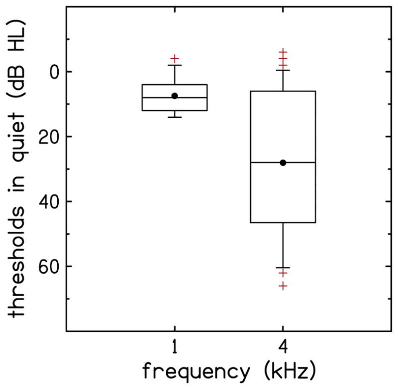
Audiometric thresholds at 1 kHz and 4 kHz for the participants of the study. The lower and upper margins of the boxes represent the 25^th and 75^th percentiles, respectively. The lower and upper whiskers represent the 10^th and 90^th percentiles, respectively. The line within the box represents the median, the filled circles represent the mean, and the plus signs indicate outliers, i.e., points that lie outside the 10^th-to-90^th percentile range.

Figure 2 shows representative ABR waveforms from one participant with SNHL, for 1 kHz (A) and 4 kHz (B). Each waveform is the average of four individual recordings for each stimulus condition. In each panel, the solid line is the response when the stimulus level was 100 dB peSPL and the dashed line is the response when the stimulus level was 80 dB peSPL. Locations of the SP, AP peak and the baseline that was used as reference in the calculations of SP and AP amplitudes are indicated in the waveform for 1 kHz at 100 dB peSPL (A). The SP was defined as the shoulder preceding the AP peak. Also indicated are peaks and troughs for ABR Waves I and V. For this example, the baseline was selected as the midpoint of the alternating-current (AC) signal (presumably either stimulus artifact or cochlear microphonic) at the early portion of the waveform. The baseline for the 1-kHz waveform (A) at 100 dB SPL, at 0.7 ms, is indicated using an open circle. ABR and ECochG components are also evident in the waveform for 4 kHz (B); however, they are not indicated to avoid clutter.

FIG. 2.

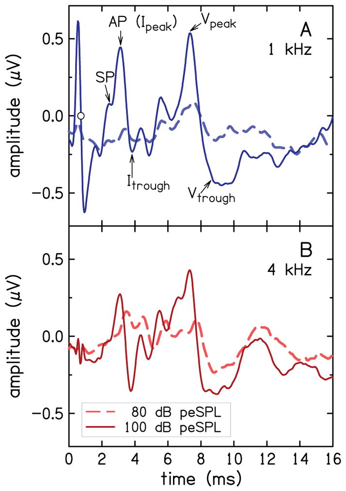
ABR waveforms for a representative participant for waveforms for 1 kHz (A) and 4 kHz (B). In each panel, waveforms are shown for 100 dB peSPL (solid line) and 80dB peSPL (dashed line). The AP, SP and the baseline (circle symbol at 0.7 ms), as well as the peaks and troughs of ABR Waves I and V, are identified in A. The peak at 0.6 ms is stimulus artifact.

The distribution of NEB values (rounded to the nearest integer) are shown in Fig. 3 in the form of a stacked histogram. The NEB has a theoretical range of 64 to 95.5 L_Aeq8760h (Stamper and Johnson, 2015a). In this study, NEB values ranged from 66.8 to 86.5 (mean = 75.2, SD = 5.4) L_Aeq8760h across all participants. The range of NEB values was 66.8 to 80.3, (mean = 73.2, SD = 4.5) L_Aeq8760h for female participants, and 67.5 to 86.5 (mean = 77.4, SD = 5.5) L_Aeq8760h for male participants. That is, the male participants had higher amounts of noise exposure than the female participants; however, the difference was not statistically significant (t(15)=−2.0, p=0.06). Eight of the 16 male participants and only two of the 17 female participants had NEB values (≥ 79) that are considered representative of high noise-exposure backgrounds. The ranges of NEB values from our study are similar to those observed in previous studies that utilized the NEQ to assess noise-exposure history. Specifically, Megerson (2010) reported ranges of 64–84 LAeq8760h for females and 64–88 LAeq8760h for males, and Stamper and Johnson (2015a) reported ranges of 67–83 LAeq8760h for females and 70–82 LAeq8760h for males.

FIG 3.

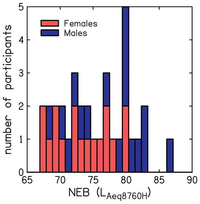
Distribution of noise exposure background (NEB) for female and male participants.

Figure 4 shows the SNR of the TEN (HL) test as a function of audiometric threshold in quiet, for 1 kHz (A) and 4 kHz (B). SNR was calculated as the difference between thresholds in noise and the level of the noise masker (70 dB HL). In each panel, solid lines are the simple linear regression fit to the data and dashed lines are the 95% confidence bounds. Note that some participants required a negative SNR to detect the tone (i.e., they were able to detect the tone when its level was lower than the level of the TEN masker), while others could only detect the tone when the SNR was positive. There was a correlation between thresholds in quiet and SNR at both 1 kHz (r=0.49, p<0.01) and 4 kHz (r=0.65, p<0.01). That is, a portion of the variance in thresholds in noise is due to hearing thresholds. Removing this component of the total variance provides the basis for our definition of a proxy for HHL.

FIG. 4.

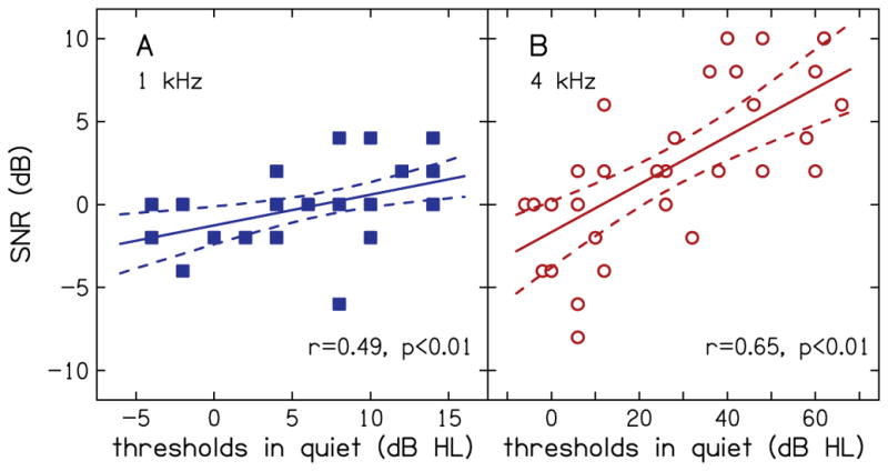
SNR for TEN (HL) test as function of audiometric thresholds in quiet for 1 kHz (A) and 4 kHz (B). Solid lines are the simple linear regression fits to the data and dashed lines are the 95% confidence bounds.

Figure 5 shows the threshold in noise residual (TINR), i.e. SNR residual, as a function of thresholds in quiet. Data were plotted using the same conventions that were used in Fig. 4. Figure 5 is equivalent to a rotation of Fig. 4 such that the slope of the regression line is zero (indicating a lack of a relationship between threshold in noise residual and threshold in quiet). Thresholds-in-noise residual is negative valued for SNRs that were below the regression line and positive valued for SNRs that were above the regression in Fig. 4. The 95% confidence bounds divide the range of TINR into three distinct regions. Based on TINR and the confidence bounds, participants above the 95% percentile bound (seven at 1 kHz and 11 at 4 kHz) have suprathreshold processing deficits, participants below the 5% percentile bound do not have suprathreshold processing deficits, and participants within the confidence bounds have an indeterminate status. Note the lack of a relationship between the status of suprathreshold processing ability and thresholds in quiet. This supports the idea that synaptopathy may exist not only in listeners with NH but also in listeners with SNHL.

FIG. 5.

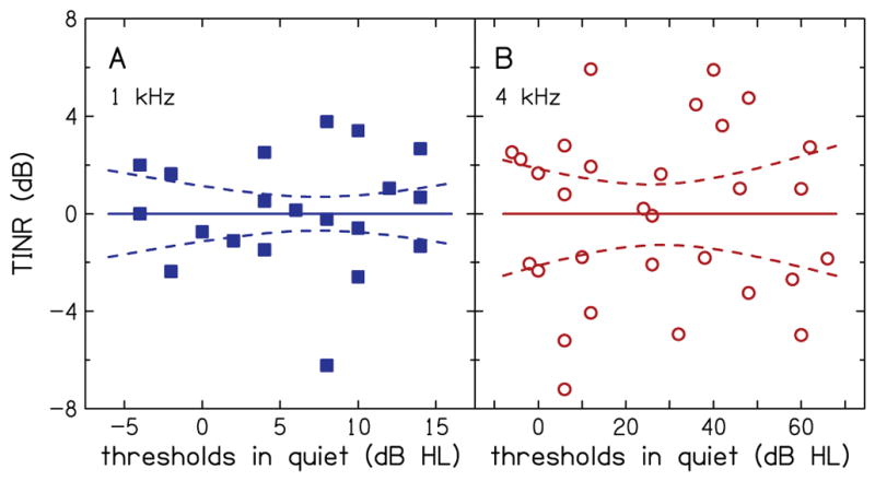
Thresholds in noise residual (TINR) as function of audiometric thresholds in quiet for 1 kHz (A) and 4 kHz (B). Solid lines are the simple linear regression fit to the data and dashed lines are the 95% confidence bounds.

Pairwise correlational analysis

In addition to thresholds in noise, thresholds in quiet were correlated with several other explanatory measures. These are summarized using values of r and p-values in Table 2. Bold font indicates correlations for which p<0.05. Including SNR for the TEN test, correlations with p<0.05 were observed for seven of 21 variables at 1 kHz and for 9 variables at 4 kHz. Correlations with thresholds in quiet for which p<0.05 at both 1 and 4 kHz were observed for five variables: SNR for the TEN test, age, DPOAE level, L_{10 CU} (lower segment of the CLS function) and Wave I amplitude at 100 dB peSPL. Correlation between thresholds in quiet and age was expected (Robinson & Sutton 1978; Brant & Fozard 1990; Lee et al. 2005). Correlations of thresholds in quiet with DPOAE level and with L_{10 CU} were also expected because these measures reflect OHC function, which relates to audiometric thresholds. Correlation between DPOAE level and L10 CU at 4 kHz (r =0.72, p<0.01; not reported in Table 2) suggests that the correlation of the three measures that reflect OHC function with each other is driven by individual differences in OHC function, and not by measurement noise. DPOAE level and the lower portion of the CLS function, however, were not correlated at 1 kHz (r =0.18, p=0.34). This is likely due to higher measurement noise for DPOAE measurements at 1 kHz compared to 4 kHz (the average noise floor was −14.89 and −22.94 dB at 1 and 4 kHz, respectively). This may also be due to the smaller variability in both DPOAE and CLS data at 1 kHz (where all participants had thresholds within the normal range) compared to 4 kHz. Across all participants, SDs for DPOAE and CLS were 6.93 dB and 10.41 dB at 1 kHz, and 13.39 dB and 16.81 dB at 4 kHz. The lack of a correlation of thresholds in quiet with the AP amplitude, when there was a correlation with Wave I amplitude, may be due to differences in the methods used to calculate the AP and Wave I amplitudes. Recall that while the peaks for the AP and ABR Wave I were identical, the amplitude of the AP was calculated with reference to a baseline and the amplitude of Wave I was calculated with reference to the following trough. Data for variables for which correlations with thresholds in quiet had p<0.05 at both 1 and 4 kHz are plotted in Fig. 6 with closed squares and open circles indicating data at 1 and 4 kHz, respectively.

Table 2.

Correlation of audiometric thresholds in quiet with explanatory variables at 1 and 4 kHz. Bold font indicate correlations with p<0.05. Subscripts 80 and 100 indicate stimulus level in dB peSPL.

Variable	1 kHz		4 kHz
	r	p	r	p
Sex	0.06	0.75	0.10	0.58
Age	0.74	<0.01	0.67	<0.01
DPOAE level	0.41	0.02	0.86	<0.01
L10 CU	0.36	0.04	0.89	<0.01
L40 CU	0.01	0.94	0.19	0.29
Wave I80	0.33	0.40	0.41	0.03
Wave I100	0.48	0.01	0.58	<0.01
Wave I difference	0.62	0.01	0.38	0.05
Wave V80	0.14	0.42	0.53	<0.01
Wave V100	0.11	0.55	0.37	0.05
Wave V/Wave I ratio80	0.34	0.83	0.59	0.71
Wave V/Wave I ratio100	0.48	0.01	0.19	0.81
SP/AP ratio80	0.46	0.36	0.32	0.20
SP/AP ratio100	0.41	0.11	0.14	0.50
SP80	0.29	0.57	0.01	0.98
SP100	0.34	0.16	0.34	0.10
AP80	0.22	0.57	0.27	0.21
AP100	0.37	0.06	0.49	0.01
AP difference	0.45	0.26	0.44	0.03
LAeq8760h	0.20	0.27	0.16	0.40
Thresholds in noise	0.49	<0.01	0.65	<0.01

FIG. 6.

Relationship of audiometric thresholds in quiet with measured variables at 1 kHz (closed squares) and 4 kHz (open circles) with correlations having p<0.05 at both frequencies. Correlations with p<0.05 were observed for age (A), DPOAE level (B), L_{10 CU} (C), and Wave I amplitude at 100 dB peSPL (D).

In the exploratory pairwise correlational analysis to determine the relationship between thresholds-in-noise residual and explanatory variables, thresholds-in-noise residual at 1 kHz was correlated with the residual of the SP/AP ratio at 100 dB peSPL (r=0.58, p=0.01). At 4 kHz, thresholds-in-noise residual was correlated with the residual of sex (r=0.37, p=0.04), with females having a higher thresholds-in-noise residual than males. For the differential analysis, thresholds-in-noise residual was correlated with the residuals of Wave I amplitude (r=0.43, p=0.02) and Wave V amplitude (r=0.55, p<0.01), both at 100 dB peSPL. The data for these residuals (having correlation of p<0.05) are plotted in Fig. 7, where thresholds-in-noise residual is plotted on the abscissa. For the differential analysis, the quantity in the ordinate axes is the ratio of the value of variable at 4 kHz to the value of variable at 1 kHz. The SP/AP ratio (Fig. 7A) increased with the amount of thresholds-in-noise residual, reflecting an increase in the SP and a decrease in the AP with thresholds-in-noise residual, although both SP and AP were not significantly correlated with thresholds-in-noise residual. The trends in our data, i.e. SP/AP ratio emerging as a possible indicator of suprathreshold processing deficit, are similar to trends in the Liberman et al. (2016) study, where the SP/AP ratio was an indicator of suprathreshold processing deficit. The trend that the residual of the SP amplitude increases with thresholds-in-noise residual is also consistent with Liberman et al. (2016), who observed an elevated SP in listeners with high noise-exposure history, and with Kim et al. (2005), who observed an increase in the SP after exposure to music at levels that were high enough to cause temporary threshold shifts exceeding 5 dB. However, as stated earlier in Methods section, caution should be made when interpreting our preliminary data because a correction was not applied for multiple comparisons.

FIG. 7.

Relationship of thresholds-in-noise residual (TINR) with residuals of explanatory variables having correlations with p<0.05. Correlations with p<0.05 were observed for SP/AP ratio at 1 kHz and 100 dB peSPL (A), sex at 4 kHz (B), Wave I amplitude at 100 dB peSPL for the differential analysis (C), and Wave V amplitude at 100 dB peSPL for the differential analysis (D). The differential analysis utilized the ratios of the value of variables at 4 kHz to the value of the variables at 1 kHz.

Although the raw sex variable was coded as Male = 1, and female =−1, calculating the residual sex variable created a spread around these values (Fig. 7B). The higher thresholds-in-noise residual in females compared to males was not expected because males are more likely to have higher occupational noise exposure and are more likely to engage in recreational activities where noise exposure might be high. This result was also in contrast with amount of noise exposure, as assessed using the NEQ (Fig. 3), where males had higher amounts of noise exposure than females, although the relationship was not statistically significant (t(15)=−2.0, p=0.06). Correlation of thresholds-in-noise residual with residual of Wave I amplitude ratio (Fig. 7C) was expected since this variable reflects ANF integrity. The increase in thresholds-in-noise residual with Wave I amplitude ratio suggests greater neural loss at 4 kHz. The lack of a correlation of thresholds-in-noise residual with AP amplitude, when there was a correlation with Wave I amplitude, was unexpected and may have been a result of the way in which the AP was quantified. Recall that while the peaks for the AP and ABR Wave I were identical, the amplitude of the AP was calculated with reference to a baseline and the amplitude of Wave I was calculated with reference to the following trough. There was less uncertainty in amplitude estimates referenced to the more reliably observed trough, compared to less reliably observed baseline preceding the AP, which may have contributed to the differences in correlations.

Contrary to our predictions, the NEB was not correlated with the AP, ABR Wave I, SP/AP ratio or thresholds-in-noise residual at both 1 and 4 kHz. The lack of a relationship between noise-exposure estimate and ABR Wave I amplitude disagrees with the data reported by Stamper and Johnson (2015a) and Bramhall et al. (2017), who observed statistically significant relationships. The stimulus level required for loudness judgments of 40 CU, L_{40 CU} was correlated with the amplitude difference between Wave V and Wave I (r = 0.46, p=0.02) at 4 kHz and 80 dB SPL.

Multiple linear regression model

As a preliminary validation of the MLR model for HHL, predictions of thresholds-in-noise residual were made using the model with the residuals of the explanatory variables, including audiometric thresholds in quiet, sex, and age as inputs. Separate models to predict thresholds-in-noise residual at 1 and 4 kHz were created with each model utilizing explanatory variables at both frequencies. Figure 8 demonstrates the effect of the number of principal components of the PCA on the MLR models for 1 and 4 kHz. Specifically, Fig. 8A shows the average (over the 1000 simulations) amount of variance of the residual variables that is explained by the PCs as the number of components is varied from four to 20. Recall that the PCs were ordered and included in the model according to the amount of variance accounted for by each component (largest to smallest). Because the same explanatory variables served as predictors in the models for 1 and 4 kHz, the variance explained is the same at both frequencies, and thus only one curve is plotted. Fig. 8B shows values of r for the correlation between the predicted thresholds-in-noise residual (outcome of MLR model) and measured thresholds-in-noise residual (residual of the SNR for the TEN (HL) test) as the number of PCs is varied. Finally, Fig. 8C shows the slope of the simple linear regression fit to the predicted thresholds-in-noise residual versus measured thresholds-in-noise residual as the number of PCs is varied. As expected, the variance explained increases as the number of PCs increases. The values of r and slope also increase with number of PCs, with larger values of both metrics at 1 kHz compared to 4 kHz.

FIG. 8.

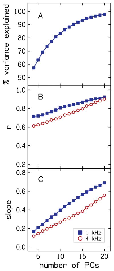
Effect of number of PCs on variance of explanatory variables explained by PCs (A), and on MLR model predictions as characterized using r (B) and slope of simple linear regression fit to the data (C). Data for 1 and 4 kHz are plotted using closed squares and open circles, respectively.

An example of the predicted thresholds-in-noise residual is plotted as a function of measured thresholds-in-noise residual in Fig. 9 for a condition in which the number of PCs (nine) is such that the variance explained by the PCs first exceeds 80% (mean = 80.3%, SD = 5.64, range = 70.5 to 100%, over the 1000 simulations). This model balances predictive power with number of components used. Pearson correlation was r = 0.78 (p<0.01) at 1 kHz (A) and r = 0.69 (p<0.01) at 4 kHz (B). The correlation coefficients translate into variances accounted for of 61% and 48%. The slopes of the simple linear regression fit to the data were 0.35 and 0.24, at 1 kHz and 4 kHz, respectively.

FIG. 9.

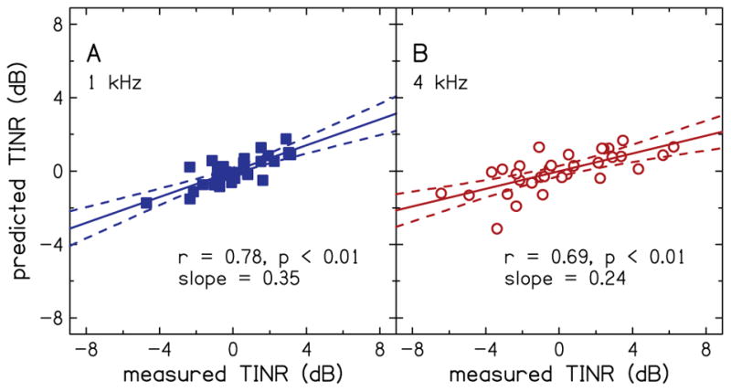
Example of the prediction of thresholds-in-noise residual (TINR) using a combination of principal component analysis with nine principal components and multiple linear regression analysis. Predictions are shown for 1 kHz (A) and 4 kHz (B).

DISCUSSION

Noise-induced synaptopathy may be a cause of suprathreshold processing difficulties in humans. As a first step toward understanding noise-induced suprathreshold processing deficits, this study developed a preliminary model of HHL, in which the residual of thresholds in noise served as the outcome variable. ABR, ECochG, DPOAE, and CLS measurements served as explanatory variables reflecting functional integrity of sites along the auditory pathway. Our hypothesis was that performance on the thresholds-in-noise task is influenced by synaptopathy because performance on this task depends on the integrity of IHCs and ANFs. A unique and potentially important aspect of the present study is the development of a functional and quantitative estimate of HHL as the portion of the variance in thresholds in noise that is not accounted for by thresholds in quiet (i.e. thresholds-in-noise residual). Thresholds-in-noise residual has intuitive appeal as a proxy for HHL because it is (by definition) not correlated with thresholds in quiet. However, other factors may also contribute to the variance in the residual, including aging, sex and cognitive-processing deficits (e.g. Hornsby 2013; Edwards 2016). Our use of the variance in suprathreshold measures (thresholds in noise in the current study) that is not accounted for by audiometric thresholds as a proxy for HHL can be extended to both listeners with normal hearing and listeners with hearing loss because both groups can have suprathreshold processing deficits. That is, a group of listeners with identical audiograms (normal hearing or hearing impaired) can have varied performance on a suprathreshold auditory task. Thus, in some individuals, it is possible that a combination of both “unhidden” and hidden hearing loss exists. This has implications for expected benefits from amplification, which may lead to different rehabilitation strategies for those with only OHC loss and those with OHC loss and synaptopathy.

Methodological Limitations

Our electrode configuration for ABR and ECochG measurements (ear-canal electrode and surface electrodes at the vertex and on the high forehead) enhanced Wave I and the SP. This enabled us to measure Wave I in 31 of 33 participants at both 1 kHz and 4 kHz when the stimulus level was 100 dB peSPL (see Table 1). However, Wave I was more difficult to observe at the lower stimulus level (80 dB peSPL), with 16 of 33 and 27 of 32 participants having measurable Wave I at 1 and 4 kHz, respectively. The SP was even more difficult to measure at 80 dB SPL, with only six participants having a measurable SP at 1 kHz. Still, our ability to measure Wave I, AP and SP was encouraging because these potentials are considered difficult to measure (e.g. Mehraei et al. 2016).

The use of two methods for identifying the baseline of ABR/ECochG waveforms may have contributed to the variability in SP amplitude. The use of two methods was necessitated by the fact that it was not always possible to identify a stimulus artifact or cochlear microphonic (which was used to define the baseline) in some waveforms. In the future, use of a slower repetition rate (e.g. 11/s) may help in the selection of a baseline because the longer inter-stimulus interval (91 ms at 11/s versus 37 ms at the 27/s repetition rate that was used) would allow additional time for the response to the previous stimulus to decay before the next stimulus is presented. A slower repetition rate would also allow for use of higher stimulus levels as there would be less stimulus energy over time.

In the current study, thresholds in noise were measured using the TEN (HL) test. This test was selected because simple procedures exist that utilize audiometric techniques. However, the limited bandwidth of the TEN (HL) masker (bandwidth of about 4 kHz) limits the application of this test to frequencies ≤ 4 kHz. In future studies, a three-interval forced choice adaptive procedure will be utilized to provide more accuracy compared to audiometric procedures, and use of a masker with a broader bandwidth will allow for measurements at high frequencies (> 4 kHz).

Correlational Analysis Suggests That ABR and ECochG Measures May Be Useful Indicators of HHL

In exploratory analyses, thresholds-in-noise residual was correlated with the residuals of some of the measures that reflect IHC and ANF integrity (SP/AP ratio at 1 kHz, and ABR Waves I and V for the differential analysis; Fig. 6). Although these correlations were observed for a limited set of stimulus conditions, they provide a preliminary validation of our methods for obtaining a proxy for HHL. Correlation of thresholds-in-noise residual with the SP/AP ratio at 1 kHz when there was no correlation with Wave I or AP residuals at the same frequency is likely because the ratio between the SP and AP eliminated some of the inter-subject variability of human ECochG measures (e.g., differences in head size, electrode contact). Correlation of thresholds-in-noise residual with ABR Waves I and V residuals for the differential analysis when correlations were not observed for 1 and 4 kHz highlights the importance of differential analysis for controlling inter-subject variability (Bharadwaj et al 2014; Plack et al. 2016).

The observation that SP/AP ratio increased with the amount of thresholds-in-noise residual was due to an increase in the SP amplitude and a decrease in the AP amplitude. The trend in the changes of the SP amplitude and SP/AP ratio with thresholds-in-noise residual are consistent with previous studies of noise exposure in humans (Liberman et al. 2016; Kim et al. 2005). Liberman et al. 2016 speculated that the increase in SP amplitude with amount of noise exposure was due to contributions from non-linear components in the receptor potentials from IHCs and/or OHCs, and excitatory post-synaptic potentials from cochlear-nerve terminals under IHCs.

We hypothesized that variability in the upper segment of the CLS function (quantified using L_{40 CU}) was partly driven by IHC and ANF integrity because it is presumably not related to OHC function. In exploratory analyses, L₄₀ CU was correlated with the amplitude difference between Wave V and Wave I, but not with Wave I itself. The lack of a correlation with Wave I may be a reflection of our small sample size. It is also possible that the variability in the upper segment of the CLS function is influenced by factors other than IHC and ANF integrity, such as cognitive factors which were not evaluated in the present study.

Limitations of Noise-Exposure Questionnaires

Noise-exposure history, as assessed by the NEQ, was not correlated with thresholds-in-noise residual or ABR Wave I amplitude. This finding is in contrast to observations of Stamper & Johnson (2015a) and Bramhall et al (2017), who found a relationship between noise-exposure history and Wave I amplitude, but in agreement with studies by Prendergast et al. (2017), and Spankovich et al. (2017), who found no relationship between these same variables. In addition, Yeend et al. (2017) found no relationship between lifetime noise exposure and performance on auditory processing and speech-in-noise tests. The lack of a relationship between noise-exposure history and measures that reflect ANF integrity in the current study and the disagreement across studies stems, in part, from the use of questionnaires to assess noise-exposure history. Since studies in which noise exposure is experimentally controlled are not possible in humans, questionnaires have been used, despite their subjective nature. These questionnaires, however, may not be reliable at quantifying noise-exposure history. The lack of a relationship between noise-exposure history and measures that reflect ANF integrity in the current study may also be a due to the small sample size. Perhaps a relationship would have been observed with a larger number of participants. A relationship may also have been observed if the questionnaire used in the current study assessed exposure to noise produced by firearms, given that Bramhall et al. showed a relationship between firearm use and ABR wave I amplitude. It is also possible that a lack of reliable relationships in the current study could reflect the lack of any real relationships between the measurements. It is worth noting that several other studies did not observe relationships between behavioral and physiological measures that were hypothesized to be predictive of HHL (e.g., Prendergast et al. 2017; Grose et al. 2016; Spankovich et al. 2017; Yeend et al. 2017). It is also possible that noise-induced HHL may not be prevalent in humans because typical occupational and recreational noise exposures are not high enough to cause synaptopathy. Less than half of the study participants (eight of the 16 male participants and only two of the 17 female participants) had noise exposure backgrounds that are considered high according to the NEQ. This highlights the difficulty of describing HHL in humans. Anecdotally, some patients report difficulty hearing in noise that would not be predicted from their pure-tone audiogram. Thus, unexplained difficulties in suprathreshold function remains a clinical concern.

Overall, we observed higher thresholds-in-noise residual in females compared to males, which was not expected because males are more likely to have higher noise exposure than females. This result was also in contrast with amount of noise exposure, as assessed using the NEQ, where the results for males suggested higher amounts of noise exposure than females. We assessed the extent to which differences in age between our male and female participants could explain the higher thresholds-in-noise residual in females. Aging has been shown to cause synaptopathy that is similar to that caused by noise exposure (Sergeyenko et al. 2013; Kujawa & Liberman 2015). The age of our female participants (mean = 43.3, SD = 11.5, range = 23 to 64 years) was similar to that our male participants (mean = 40.9, SD = 12.3, range = 23 to 59 years). In addition, age and sex were not related. Thus, differences in age cannot explain the higher thresholds-in-noise residual that we observed in our female participants.

Statistical Modeling May Provide a Verifiable and Quantifiable Estimate of HHL

Although exploratory correlational analysis is useful for detecting patterns in the data, it is inconsequential to the success of the MLR model. Unlike correlational analysis, MLR leverages and combines the predictive power of several measures, some of which are weakly correlated with thresholds-in-noise residual when considered in isolation, to produce more robust predictions. Our model of HHL predicted thresholds-in-noise residual at a statistically significant level, as shown in Fig. 9 at a statistically significant level. Variance accounted for by the model’s predictions were 61% and 48% at 1 and 4 kHz, respectively. The model, however, is limited by the reliability of all measures, especially estimates of noise exposure (derived from the NEQ), lack of a gold standard for HHL, the generally smaller variance due to thresholds-in-noise residual compared to unhidden SNHL, and the relatively small sample size (especially in relation to the number of variables). Cognitive processing may also have influenced the results of our behavioral outcome measure – thresholds in noise. Additionally, the accuracy of the model was limited by missing data (see Table 1), which necessitated the use of the alternating least squares algorithm in the PCA. This algorithm uses an iterative process with random initial value to estimate the missing values. In future studies, having complete data from each participant will eliminate the need for the alternating least squares algorithm in the PCA. Reducing the number of explanatory variables and utilizing a large sample may reduce or eliminate the need to reduce the dimensionality of the data using PCA, while improving prediction accuracy. Application of the model to an independent group of participants will provide further validation of the modelling approach.

For the example presented in Fig. 9, the model under-predicted the magnitude of thresholds-in-noise residual (i.e. slope was less than unity). However, in Fig. 8 the slope increased towards unity as the number of PCs increased. This, together with the fact that Pearson correlation also increased with the number of PCs, suggests that the prediction accuracy of the model may be improved if either the number of participants increases, or the number of explanatory variables decreases, or a combination of the two factors.

Our model of HHL utilized a behavioral measure (thresholds in noise) as an outcome variable and physiological (ECochG, ABR and DPOAE) and behavioral (CLS) measures as explanatory variables. Several physiological measures, such as middle-ear muscle reflex, medial olivocochlear reflex and frequency-following response may be predictive of HHL, as described earlier. Using these measures as outcome variables and only physiological measures as explanatory variables would allow for objective identification of HHL We assessed the accuracy of the current model when only physiological measures were used as explanatory variables. The variance accounted for by the prediction fell from 61% to 48% at 1 kHz and from 48% to 36% 4 kHz; thus the behavioral data contributed to the accuracy of the predictions.

It is possible that other behavioral measures may be more sensitive to the presence of HHL than thresholds in noise. For example, studies have shown a relationship between measures that are thought to reflect HHL and behavioral measures of temporal-coding abilities, such as frequency-modulation detection threshold (Johannesen et al, 2016), and spatial selective auditory attention (Ruggles et al. (2011). A relationship has also been shown between measures that are thought to reflect HHL and performance on speech-in-noise tests (Liberman et al. 2016). Future studies are needed that explore these measures as outcome variables in the model of HHL.

Translation of Animal Studies to Humans, and Clinical Implications

The current study was motivated by observations in animal studies implicating damage to the peripheral auditory system (IHCs, synapses and low-SR ANFs) as a primary cause of HHL. Several issues have to be considered in efforts to translate these findings to humans (see Dobie and Humes, 2017 and Hickox et al. 2017 for reviews). There may be species differences in susceptibility to noise. Humans may be more susceptible to impulsive noise, such as firearms, than to the continuous noise that was shown to cause synaptopathy in laboratory animals. It may be that the controlled higher noise levels that were used in animal studies are required to cause synaptopathy in humans. In studies of temporary threshold shift (TTS), levels that caused TTS in laboratory animals were lower than those that caused TTS in humans (e.g. Mills et al. 1979). The lack of experimental control of noise experienced by humans might mean that humans may have other cochlear dysfunctions (i.e. loss of OHC, IHC) in addition to synaptopathy, making it more difficult to identify synaptopathic HHL. Neurophysiological differences between species also have to be considered. Joris et al. (2011) suggested that the relationship between spontaneous firing rate and thresholds of ANFs maybe be different in non-human primates (macaque) compared to animals commonly used in laboratory studies (guinea pig, mouse, gerbil, cat). More research is needed to address these issues.

Currently, clinical intervention strategies for HHL do not exist. The lack of interventions is driven, in part, by the lack of diagnostic tools for HHL, as well as other technological limitations. Our statistical modeling approach may establish a theoretical framework for the development of diagnostic tools to identify HHL. The ability to diagnose HHL may usher in new methods for clinical evaluation, and may lead to better remediation of both SNHL and HHL. For example, studies have shown clinicians might elect to use individualized hearing-aid compression parameters if they knew that a patient had IHC dysfunction comorbid with OHC dysfunction. Additional counseling could be provided to patients diagnosed with HHL when they complain of difficulty understanding speech in noisy environments or report they are not receiving sufficient benefit from hearing aids. There is also the possibility that HHL may be managed using advanced signal-processing strategies that go beyond wide-dynamic range compression and noise reduction. A diagnosis that suggests primary neural degeneration might be treated by application of neurotrophin therapies in humans, which have been shown to regenerate synapses following noise-induced synaptopathy in transgenic mice (Wan et al. 2014; Suzuki et al. 2016). The modeling approach may also lead to applications in tinnitus research, as it has been suggested that both HHL and tinnitus share a similar underlying cause (i.e., ANF damage; Schaette & McAlpine 2011). Finally, modeling may lead to applications in aging research because aging is known to cause synaptopathy that is similar to that caused by noise exposure (Sergeyenko et al. 2013; Kujawa & Liberman 2015).

CONCLUSIONS

Measures of thresholds in noise, the SP/AP ratio, and ABR Waves I and V may be useful for the prediction of HHL in humans. These results are consistent with the view that IHC and ANF pathology may underlie suprathreshold auditory performance. Our approach of quantifying HHL as the variance that remains in suprathreshold measures of auditory function after removing the variance due to thresholds in quiet may provide a verifiable and quantifiable estimate of HHL. The predictive power of our statistical modeling suggests that this approach may provide a framework for the development of diagnostic tools to identify HHL in humans.

References

- Abdala C, Visser-Dumont L. Distortion product otoacoustic emissions: A tool for hearing assessment and scientific study. Volta Rev. 2001;103:281–302. [PMC free article] [PubMed] [Google Scholar]
- Al-Salim SC, Kopun JG, Neely ST, et al. Reliability of categorical loudness scaling and its relation to threshold. Ear Hear. 2010;31:567–578. doi: 10.1097/AUD.0b013e3181da4d15. [DOI] [PMC free article] [PubMed] [Google Scholar]
- Bharadwaj HM, Verhulst S, Shaheen L, et al. Cochlear neuropathy and the coding of supra-threshold sound. Front Syst Neurosci. 2014;8:26. doi: 10.3389/fnsys.2014.00026. [DOI] [PMC free article] [PubMed] [Google Scholar]
- Bharadwaj HM, Masud S, Mehraei G, et al. Individual differences reveal correlates of hidden hearing deficits. J Neurosci. 2015;35:2161–2172. doi: 10.1523/JNEUROSCI.3915-14.2015. [DOI] [PMC free article] [PubMed] [Google Scholar]
- Bramhall NF, Konrad-Martin D, McMillan GP, et al. Auditory brainstem response altered in humans with noise exposure despite normal outer hair cell function. Ear Hear. 2017;38:e1–e12. doi: 10.1097/AUD.0000000000000370. [DOI] [PMC free article] [PubMed] [Google Scholar]
- Brand T, Hohmann V. Effect of hearing loss, center frequency, and bandwidth on the shape of loudness functions in categorical loudness scaling. Audiol. 2001;40:92–103. [PubMed] [Google Scholar]
- Brant LJ, Fozard JL. Age changes in pure-tone hearing thresholds in a longitudinal study of normal human aging. J Acoust Soc Am. 1990;88:813–820. doi: 10.1121/1.399731. [DOI] [PubMed] [Google Scholar]
- Brownell WE. Outer hair cell electromotility and otoacoustic emissions. Ear Hear. 1990;11:82–92. doi: 10.1097/00003446-199004000-00003. [DOI] [PMC free article] [PubMed] [Google Scholar]
- Chen Z, Hu G, Glasberg BR, Moore BC. A new method of calculating auditory excitation patterns and loudness for steady sounds. Hear Res. 2011;282:204–215. doi: 10.1016/j.heares.2011.08.001. [DOI] [PubMed] [Google Scholar]
- Chertoff ME, Earl BR, Diaz FJ, et al. Analysis of the cochlear microphonic to a low-frequency tone embedded in filtered noise. J Acoust Soc Am. 2012;110(132):3351–3362. doi: 10.1121/1.4757746. [DOI] [PMC free article] [PubMed] [Google Scholar]
- Costalupes JA, Young ED, Gibson DJ. Effects of continuous noise backgrounds on rate response of auditory nerve fibers in cat. J Neurophysiol. 1984;51(6):1326–1344. doi: 10.1152/jn.1984.51.6.1326. [DOI] [PubMed] [Google Scholar]
- Costalupes JA. Representation of tones in noise in the responses of auditory nerve fibers in cats. I Comparison with detection thresholds. J Neurosci. 1985;5(12):3261–3269. doi: 10.1523/JNEUROSCI.05-12-03261.1985. [DOI] [PMC free article] [PubMed] [Google Scholar]
- Dobie RA, Humes LE. Commentary on the regulatory implications of noise-induced cochlear neuropathy. International J Aud. 2017;56(sup1):74–78. doi: 10.1080/14992027.2016.1255359. [DOI] [PubMed] [Google Scholar]
- Durrant JD, Wang J, Ding DL, Salvi RJ. Are inner or outer hair cells the source of summating potentials recorded from the round window? J Acoust Soc Am. 1998;104:370–377. doi: 10.1121/1.423293. [DOI] [PubMed] [Google Scholar]
- Edwards B. A Model of Auditory-Cognitive Processing and Relevance to Clinical Applicability. Ear Hear. 2016;37:85S–91S. doi: 10.1097/AUD.0000000000000308. [DOI] [PubMed] [Google Scholar]
- El-Badry MM, McFadden SL. Electrophysiological correlates of progressive sensorineural pathology in carboplatin-treated chinchillas. Brain Res. 2007;1134:122–130. doi: 10.1016/j.brainres.2006.11.078. [DOI] [PMC free article] [PubMed] [Google Scholar]
- Ferraro JA, Durrant JD. Electrocochleography in the evaluation of patients with Meniere’s disease/endolymphatic hydrops. J Am Acad Audiol. 2006;17:45–68. doi: 10.3766/jaaa.17.1.6. [DOI] [PubMed] [Google Scholar]
- Furman AC, Kujawa SG, Liberman MC. Noise-induced cochlear neuropathy is selective for fibers with low spontaneous rates. J Neurophysiol. 2013;110:577–586. doi: 10.1152/jn.00164.2013. [DOI] [PMC free article] [PubMed] [Google Scholar]
- Gorga MP, Neely ST, Ohlrich B, et al. From laboratory to clinic: A large scale study of distortion product otoacoustic emissions in ears with normal hearing and ears with hearing loss. Ear Hear. 1997;18:440–455. doi: 10.1097/00003446-199712000-00003. [DOI] [PubMed] [Google Scholar]
- Gorga MP, Johnson TA, Kaminski JR, et al. Using a combination of click- and tone burst-evoked auditory brain stem response measurements to estimate pure-tone thresholds. Ear Hear. 2006;27(1):60–74. doi: 10.1097/01.aud.0000194511.14740.9c. [DOI] [PMC free article] [PubMed] [Google Scholar]
- Grose J, Buss E, Hall J, Hall JW. ‘Hidden Hearing Loss’ and Intense Music Exposure in Humans. Paper presented at the 39th Annual Midwinter Meeting of Association for Research in Otolaryngology; San Diego. 2016. [Google Scholar]
- Henry KS, Heinz MG. Diminished temporal coding with sensorineural hearing loss emerges in background noise. Nat Neurosci. 2012;15:1362–1364. doi: 10.1038/nn.3216. [DOI] [PMC free article] [PubMed] [Google Scholar]
- Hickox AE, Larsen E, Heinz MG, Shinobu L, Whitton JP. Translational issues in cochlear synaptopathy. Hear Res. 2017;349:164–171. doi: 10.1016/j.heares.2016.12.010. [DOI] [PMC free article] [PubMed] [Google Scholar]
- Hornsby BW. The effects of hearing aid use on listening effort and mental fatigue associated with sustained speech processing demands. Ear Hear. 2013;34:523–534. doi: 10.1097/AUD.0b013e31828003d8. [DOI] [PubMed] [Google Scholar]
- Jepsen ML, Dau T. Characterizing auditory processing and perception in individual listeners with sensorineural hearing loss. J Acoust Soc Am. 2011;129:262–281. doi: 10.1121/1.3518768. [DOI] [PubMed] [Google Scholar]
- Johannesen PT, Pérez-González P, Lopez-Poveda EA. Across-frequency behavioral estimates of the contribution of inner and outer hair cell dysfunction to individualized audiometric loss. Front Neurosci. 2014;8:214. doi: 10.3389/fnins.2014.00214. [DOI] [PMC free article] [PubMed] [Google Scholar]
- Johnson TA, Neely ST, Kopun JG, et al. Clinical test performance of distortion product otoacoustic emissions using new stimulus conditions. Ear Hear. 2010;31:74. doi: 10.1097/AUD.0b013e3181b71924. [DOI] [PMC free article] [PubMed] [Google Scholar]
- Johnson TA, Cooper S, Stamper GC, et al. Noise Exposure Questionnaire: A Tool for Quantifying Annual Noise Exposure. J Am Acad Audiol. 2017;28(1):14–35. doi: 10.3766/jaaa.15070. [DOI] [PMC free article] [PubMed] [Google Scholar]
- Joris PX, Bergevin C, Kalluri R, Mc Laughlin M, Michelet P, van der Heijden M, Shera CA. Frequency selectivity in Old-World monkeys corroborates sharp cochlear tuning in humans. Proc Natl Acad Sci. 2011;108:17516, e17520. doi: 10.1073/pnas.1105867108. [DOI] [PMC free article] [PubMed] [Google Scholar]
- Kim JS, Nam EC, Park SI. Electrocochleography is more sensitive than distortion-product otoacoustic emission test for detecting noise-induced temporary threshold shift. Otolaryngol head and neck surgery. 2005;133(4):619–24. doi: 10.1016/j.otohns.2005.06.012. [DOI] [PubMed] [Google Scholar]
- Kujawa SG, Liberman MC. Adding insult to injury: Cochlear nerve degeneration after “temporary” noise-induced hearing loss. J Neurosci. 2009;29:14077–14085. doi: 10.1523/JNEUROSCI.2845-09.2009. [DOI] [PMC free article] [PubMed] [Google Scholar]
- Kujawa SG, Liberman MC. Synaptopathy in the noise-exposed and aging cochlea: primary neural degeneration in acquired sensorineural hearing loss. Hear Res. 2015;330(Pt. B):191–199. doi: 10.1016/j.heares.2015.02.009. [DOI] [PMC free article] [PubMed] [Google Scholar]
- Kummer P, Janssen T, Arnold W. The level and growth behavior of the 2 f1−f2 distortion product otoacoustic emission and its relationship to auditory sensitivity in normal hearing and cochlear hearing loss. J Acoust Soc Am. 1998;103(6):3431–3444. doi: 10.1121/1.423054. [DOI] [PubMed] [Google Scholar]
- Lee FS, Matthews LJ, Dubno JR, et al. Longitudinal study of pure-tone thresholds in older persons. Ear Hear. 2005;26(1):1–11. doi: 10.1097/00003446-200502000-00001. [DOI] [PubMed] [Google Scholar]
- Le Prell CG, Clavier OH. Effects of noise on speech recognition: Challenges for communication by service members. Hear Res. 2016;349:76–89. doi: 10.1016/j.heares.2016.10.004. [DOI] [PubMed] [Google Scholar]
- Levine S, Margolis RH, Daly KA. Use of electrocochleography in the diagnosis of Meniere’s disease. Laryngoscope. 1998;108(7):993–1000. doi: 10.1097/00005537-199807000-00008. [DOI] [PubMed] [Google Scholar]
- Liberman MC. Auditory nerve response from cats raised in a low-noise chamber. J Acoust Soc Am. 1978;63(2):442–455. doi: 10.1121/1.381736. [DOI] [PubMed] [Google Scholar]
- Liberman LD, Liberman MC. Dynamics of cochlear synaptopathy after acoustic overexposure. J Assoc Res Otolaryngol. 2015;16(2):205–219. doi: 10.1007/s10162-015-0510-3. [DOI] [PMC free article] [PubMed] [Google Scholar]
- Liberman MC, Epstein MJ, Cleveland SC, et al. Toward a differential diagnosis of hidden hearing loss in humans. PLoS One. 2016;11:1–15. doi: 10.1371/journal.pone.0162726. [DOI] [PMC free article] [PubMed] [Google Scholar]
- Liberman MC, Kujawa SG. Cochlear synaptopathy in acquired sensorineural hearing loss: manifestations and mechanisms. Hear Res. 2017;349:138–147. doi: 10.1016/j.heares.2017.01.003. [DOI] [PMC free article] [PubMed] [Google Scholar]
- Lin HW, Furman AC, Kujawa SG. Primary neural degeneration in the guinea pig cochlea after reversible noise-induced threshold shift. J Assoc Res Otolaryngol. 2011;12:605–616. doi: 10.1007/s10162-011-0277-0. [DOI] [PMC free article] [PubMed] [Google Scholar]
- Lobarinas E, Salvi R, Ding D. Selective inner hair cell dysfunction in chinchillas impairs hearing-in-noise in the absence of outer hair cell loss. J Assoc Res Otolaryngol. 2016;17(2):89–101. doi: 10.1007/s10162-015-0550-8. [DOI] [PMC free article] [PubMed] [Google Scholar]
- Lonsbury-Martin BL, Martin GK. The clinical utility of distortion-product otoacoustic emissions. Ear Hear. 1990;11:144–154. doi: 10.1097/00003446-199004000-00009. [DOI] [PubMed] [Google Scholar]
- Lopez-Poveda EA, Johannesen PT, Merchán MA. Estimation of the degree of inner and outer hair cell dysfunction from distortion product otoacoustic emission input/output functions. Audiol Med. 2009;7:22–28. [Google Scholar]
- Lopez-Poveda EA, Johannesen PT. Behavioral estimates of the contribution of inner and outer hair cell dysfunction to individualize audiometric loss. J Assoc Res Otolaryngol. 2012;13(4):485–504. doi: 10.1007/s10162-012-0327-2. [DOI] [PMC free article] [PubMed] [Google Scholar]
- McCreery RW, Kaminski J, Beauchaine K, et al. The impact of degree of hearing loss on auditory brainstem response predictions of behavioral thresholds. Ear Hear. 2015;36(3):309–319. doi: 10.1097/AUD.0000000000000120. [DOI] [PMC free article] [PubMed] [Google Scholar]
- Megerson SC. Published Dissertation. University of Kansas; 2010. Development of a screening tool for identifying young people at risk for noise-induced hearing loss. [Google Scholar]
- Mehraei G, Hickox AE, Bharadwaj HM, et al. Auditory brainstem response latency in noise as a marker of cochlear synaptopathy. J Neurosci. 2016;36(13):3755–3764. doi: 10.1523/JNEUROSCI.4460-15.2016. [DOI] [PMC free article] [PubMed] [Google Scholar]
- Mills JH, Gilbert RM, Adkins WY. Temporary threshold shifts in humans exposed to octave bands of noise for 16 to 24 hours. J Acoust Soc Am. 1979;65(5):1238–1248. doi: 10.1121/1.382791. [DOI] [PubMed] [Google Scholar]
- Moore BC, Glasberg BR. A model of loudness perception applied to cochlear hearing loss. Aud Neurosci. 1997;3:289–311. doi: 10.1016/S0378-5955(03)00347-2. [DOI] [PubMed] [Google Scholar]
- Moore BC, Glasberg BR, Stone MA. New version of the TEN test with calibrations in dB HL. Ear Hear. 2004;25(5):478–487. doi: 10.1097/01.aud.0000145992.31135.89. [DOI] [PubMed] [Google Scholar]
- Neely ST, Liu Z. Technical Memo No 17. Boys Town National Research Hospital; Omaha, NE: 1994. EMAV: Otoacoustic emission averager. [Google Scholar]
- Oetting D, Brand T, Ewert SD. Optimized loudness-function estimation for categorical loudness scaling data. Hear Res. 2014;316:16–27. doi: 10.1016/j.heares.2014.07.003. [DOI] [PubMed] [Google Scholar]
- Plack CJ, Barker D, Prendergast G. Perceptual consequences of “hidden” hearing loss. Trends Hear. 2014;18:1–11. doi: 10.1177/2331216514550621. [DOI] [PMC free article] [PubMed] [Google Scholar]
- Plack CJ, Léger A, Prendergast G, et al. Toward a diagnostic test for hidden hearing loss. Trends Hear. 2016;20:1–9. doi: 10.1177/2331216516657466. [DOI] [PMC free article] [PubMed] [Google Scholar]
- Prendergast G, Guest H, Munro KJ, et al. Effects of noise exposure on young adults with normal audiograms I: Electrophysiology. Hear Res. 2017;344:68–81. doi: 10.1016/j.heares.2016.10.028. [DOI] [PMC free article] [PubMed] [Google Scholar]
- Rasetshwane DM, Trevino AC, Gombert JN, et al. Categorical loudness scaling and equal-loudness contours in listeners with normal hearing and hearing loss. J Acoust Soc Am. 2015;137(4):1899–1913. doi: 10.1121/1.4916605. [DOI] [PMC free article] [PubMed] [Google Scholar]
- Rasetshwane DM, Argenyi M, Neely ST, et al. Latency of tone-burst-evoked auditory brain stem responses and otoacoustic emissions: level, frequency, and rise-time effects. J Acoust Soc Am. 2013;133(5):2803–2817. doi: 10.1121/1.4798666. [DOI] [PMC free article] [PubMed] [Google Scholar]
- Reuven ML, Neely ST, Kopun JG, et al. Effect of calibration method on distortion-product otoacoustic emission measurements at and around 4 kHz. Ear Hear. 2013;34:6. doi: 10.1097/AUD.0b013e3182994f15. [DOI] [PMC free article] [PubMed] [Google Scholar]
- Richmond SA, Kopun JG, Neely ST, et al. Distribution of standing-wave errors in real-ear sound-level measurements. J Acoust Soc Am. 2011;129:3134–3140. doi: 10.1121/1.3569726. [DOI] [PMC free article] [PubMed] [Google Scholar]
- Robinson DW, Sutton GJ. Acoustics Report, Ac 84. National Physical Laboratory; Teddington: 1978. A comparative analysis of data on the relation of pure tone audiometric thresholds to age. [Google Scholar]
- Ruggles D, Bharadwaj H, Shinn-Cunningham BG. Normal hearing is not enough to guarantee robust encoding of suprathreshold features important in everyday communication. Proc Nat Acad Sci. 2011;108(37):15516–15521. doi: 10.1073/pnas.1108912108. [DOI] [PMC free article] [PubMed] [Google Scholar]
- Schaette R, McAlpine D. Tinnitus with a normal audiogram: Physiological evidence for hidden hearing loss and computational model. J Neurosci. 2011;31:13452–13457. doi: 10.1523/JNEUROSCI.2156-11.2011. [DOI] [PMC free article] [PubMed] [Google Scholar]
- Scheperle RA, Neely ST, Kopun JG, et al. Influence of in-situ sound level calibration on distortion product otoacoustic emission variability. J Acoust Soc Am. 2008;124:288–300. doi: 10.1121/1.2931953. [DOI] [PMC free article] [PubMed] [Google Scholar]
- Sergeyenko Y, Lall K, Liberman MC, et al. Age-related cochlear synaptopathy: An early-onset contributor to auditory functional decline. J Neurosci. 2013;33:13686–13694. doi: 10.1523/JNEUROSCI.1783-13.2013. [DOI] [PMC free article] [PubMed] [Google Scholar]
- Siegel JH, Hirohata ET. Sound calibration and distortion product otoacoustic emissions at high frequencies. Hear Res. 1994;80(2):146–152. doi: 10.1016/0378-5955(94)90106-6. [DOI] [PubMed] [Google Scholar]
- Spankovich C, Le Prell CG, Lobarinas E, Hood LJ. Noise history and auditory function in young adults with and without type 1 diabetes mellitus. Ear Hear. 2017 doi: 10.1097/AUD.0000000000000457. Published ahead of print. [DOI] [PubMed] [Google Scholar]
- Stover L, Gorga MP, Neely ST, et al. Toward optimizing the clinical utility of distortion product otoacoustic emission measurements. J Acoust Soc Am. 1996;100(2):956–967. doi: 10.1121/1.416207. [DOI] [PubMed] [Google Scholar]
- Stamper GC, Johnson TA. Auditory function in normal-hearing, noise-exposed human ears. Ear Hear. 2015a;36:172–184. doi: 10.1097/AUD.0000000000000107. [DOI] [PMC free article] [PubMed] [Google Scholar]
- Stamper GC, Johnson TA. Letter to the Editor: Examination of potential sex influences in Stamper, G. C., & Johnson, T. A. (2015). Auditory function in normal-hearing, noise-exposed human ears, ear hear, 36, 172–184. Ear Hear. 2015b;36:738–740. doi: 10.1097/AUD.0000000000000228. [DOI] [PMC free article] [PubMed] [Google Scholar]
- Suzuki J, Corfas G, Liberman MC. Round-window delivery of neurotrophin 3 regenerates cochlear synapses after acoustic overexposure. Sci Rep. 2016;6:24907. doi: 10.1038/srep24907. [DOI] [PMC free article] [PubMed] [Google Scholar]
- Thabet EM. Evaluation of tinnitus patients with normal hearing sensitivity using TEOAEs and TEN test. Auris Nasus Larynx. 2009;36(6):633–636. doi: 10.1016/j.anl.2009.01.002. [DOI] [PubMed] [Google Scholar]
- Thorson MJ, Kopun JG, Neely ST, et al. Reliability of distortion-product otoacoustic emissions and their relation to loudness. J Acoust Soc Am. 2012;131(2):1282–1295. doi: 10.1121/1.3672654. [DOI] [PMC free article] [PubMed] [Google Scholar]
- Valero MD, Hancock KE, Liberman MC. The middle ear muscle reflex in the diagnosis of cochlear neuropathy. Hear Res. 2016;332:29–38. doi: 10.1016/j.heares.2015.11.005. [DOI] [PMC free article] [PubMed] [Google Scholar]
- Viana LM, O’Malley JT, Burgess BJ, et al. Cochlear neuropathy in human presbycusis: Confocal analysis of hidden hearing loss in post-mortem tissue. Hear Res. 2015;327:78–88. doi: 10.1016/j.heares.2015.04.014. [DOI] [PMC free article] [PubMed] [Google Scholar]
- Vinay Hansen AS, Raen Ø, Moore BC. Reference thresholds for the TEN (HL) test for people with normal hearing. Int J Audiol. 2017:1–5. doi: 10.1080/14992027.2017.1307531. [DOI] [PubMed] [Google Scholar]
- Wan G, Gomez-Casati ME, Gigliello AR, et al. Neurotrophin-3 regulates ribbon synapse density in the cochlea and induces synapse regeneration after acoustic trauma. Elife. 2014;3:e03564. doi: 10.7554/eLife.03564. [DOI] [PMC free article] [PubMed] [Google Scholar]
- Wang J, Ding D, Salvi RJ. Functional reorganization in chinchilla inferior colliculus associated with chronic and acute cochlear damage. Hear Res. 2002;168:238–249. doi: 10.1016/s0378-5955(02)00360-x. [DOI] [PubMed] [Google Scholar]
- Wynne DP, Zeng FP, Bhatt S, et al. Loudness adaptation accompanying ribbon synapse and auditory nerve disorders. Brain. 2013;136(5):1626–38. doi: 10.1093/brain/awt056. [DOI] [PMC free article] [PubMed] [Google Scholar]
- Yeend I, Beach EF, Sharma M, Dillon H. The effects of noise exposure and musical training on suprathreshold auditory processing and speech perception in noise. Hear Res. 2017;353:224–236. doi: 10.1016/j.heares.2017.07.006. [DOI] [PubMed] [Google Scholar]
- Young ED, Barta PE. Rate responses of auditory-nerve fibers to tones in noise near masked threshold. J Acoust Soc Am. 1986;79:426–442. doi: 10.1121/1.393530. [DOI] [PubMed] [Google Scholar]