Variable importance-weighted Random Forests

Abstract

Background

Random Forests is a popular classification and regression method that has proven powerful for various prediction problems in biological studies. However, its performance often deteriorates when the number of features increases. To address this limitation, feature elimination Random Forests was proposed that only uses features with the largest variable importance scores. Yet the performance of this method is not satisfying, possibly due to its rigid feature selection, and increased correlations between trees of forest.

Methods

We propose variable importance-weighted Random Forests, which instead of sampling features with equal probability at each node to build up trees, samples features according to their variable importance scores, and then select the best split from the randomly selected features.

Results

We evaluate the performance of our method through comprehensive simulation and real data analyses, for both regression and classification. Compared to the standard Random Forests and the feature elimination Random Forests methods, our proposed method has improved performance in most cases.

Conclusions

By incorporating the variable importance scores into the random feature selection step, our method can better utilize more informative features without completely ignoring less informative ones, hence has improved prediction accuracy in the presence of weak signals and large noises. We have implemented an R package “viRandomForests” based on the original R package “randomForest” and it can be freely downloaded from http://zhaocenter.org/software.

INTRODUCTION

With the rapid development of molecular technologies, huge amount of high-throughput-omics data have been generated. These data provide rich information on various biological processes at the molecular level, and insights learned from these data may lead to new tools for disease diagnosis, prognosis, and treatment [1]. However, the large number of features in these data and the existence of complex interactions among these features pose great challenges in extracting useful information for accurate predictions. Random Forests [2], an ensemble method based on classification and regression trees (CART) trained on bootstrapped samples and randomly selected features, has been shown to have superior performance over many other classification and regression methods [2–4] and is commonly used in genomic data analyses [5,6]. However, when the number of features is very large and the signals are relatively weak, its performance tends to decline (see Results and Ref. [7] for examples).

An intuitive idea to improve the performance of Random Forests is to evaluate the importance of each feature first and then only keep the most informative ones in a second round of analysis. This is the core idea of several feature elimination Random Forests algorithms [8–10]. As a by-product of Random Forests, the variable importance score (increase in classification error rate or regression MSE when a feature is randomly permutated) [11] provides an assessment of the informativeness of each feature. The feature elimination methods utilize this measurement and iteratively select top-ranked features accordingly and re-train a Random Forests based only on selected features. While showing improvement in some cases [8–10], the main limitation of this feature elimination approach is that it is too rigid in feature selection, sensitive to inaccuracies in feature selection, and may lead to significant increase in the correlation among trees that may negatively affect the performance (see Results).

To overcome this limitation, we propose a soft “feature selection” strategy in this paper. Unlike the feature elimination approach which keeps only features with the largest importance scores, we input all the features as well as their importance scores into a second stage Random Forests model. However, in the random feature selection step when splitting a tree node, instead of sampling each feature with equal probability like Random Forests, our new method samples features according to their importance scores. With this weighted sampling strategy, the final model is able to focus on the most informative features while not completely ignoring contributions from others at the same time. We note that a similar method was proposed specifically for continuous-feature, two-class classification problems (called “enriched Random Forests”) [7]. The authors used marginal t-test (or conditional t-test [12]) q-values to guide the random feature selection. Here, we also extended this marginal testing idea to more general cases by adopting ANOVA for continuous-feature, multiple-class classification, Chi-squared test for categorical-feature classification and F-test (linear regression with only one feature) for regression.

We evaluated the performance of the proposed variable importance-weighted Random Forests (viRF), the standard Random Forests, the feature elimination Random Forests and the marginal screening-based enriched Random Forests through comprehensive simulation studies and the analysis of gene expression data sets. We found that the viRF has better performance in most cases. These results suggest that viRF is effective in using high-dimensional genomic data to construct useful predictive models.

RESULTS

Regression

Simulation models

We consider the following three models in our simulations [13].

1. y = 10sin(10πx₁) + ε, with x_i, ~ Unif (0,1), i = 1,2, …,d and ε ~ N(0,1).

2. y = 10sin(10πx₁x₂) + 20(x₃ − 0.05)² + 10x₄ + 5x₅ + ε, with x_i ~ Unif (0,1), i=1, 2, …,d and ε ~ N(0,1).

3. y = f(x) + ε, with x_i ~ Unif (0,1), i=1, 2, …, d, ε ~ N(0,1), and f(x) follows a tree structure as in Figure 1.

Figure 1.

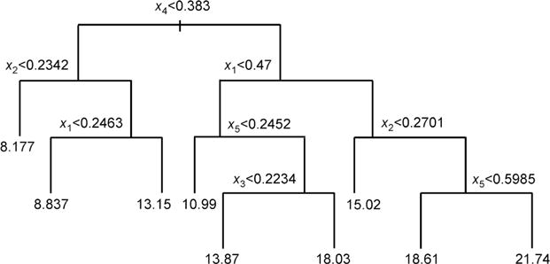
Tree structure used in regression Model 3.

The total number of features, d, was varied from 5 to 200. For each d, we generated training sets with sample size, n, ranging from 10 to 500 (Figures 2–4). The accuracy of each method was evaluated on a testing data set with 500 samples. We repeated the process 50 times and report the average MSEs, where smaller value indicates better performance.

Figure 2. MSE in regression simulation Model 1.

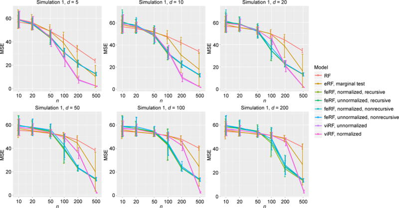
“ViRF” is short for variable importance-weighted Random Forests, “eRF” for enriched Random Forests, “feRF” for feature elimination Random Forests and “RF” for the standard Random Forests; “normalized”/“unnormalized” denotes whether the variable importance scores used are normalized, and “recursive”/“nonrecursive” denotes whether the variable importance scores are recursively estimated (see Materials and Methods for details). We adopt these notations in subsequent figures and tables.

Figure 4.

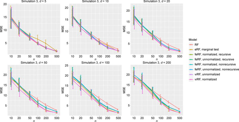
MSE in regression simulation Model 3.

In simulation Model 1, out of d total features only one (x₁) is informative. The variable importance-weighted Random Forests (viRF) and the feature elimination ones (feRF), being less influenced by noise features, both outperformed the standard Random Forests (RF) as expected (Figure 2). When sample size (n) was large relative to the dimension (d), viRFs performed better than feRFs. We also note that although linear regression was not expected to be effective for the periodic function (sin), F-test q-value based enriched Random Forests (eRF) still outperformed the standard RF in most cases (since x₁ did get smaller p-values than x₂, …, x_d). However, its performance was much worse than viRF, indicating an advantage of Random Forests’ variable importance score quantifying the feature informativeness in this scenario.

Simulation Model 2 has five informative features (x₁, …, x₅). For most d and n, all the modified Random Forests had similar performance, which were better than that of the standard RF (Figure 3).

Figure 3.

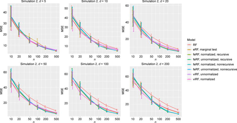
MSE in regression simulation Model 2.

For the tree structure in Model 3, with five informative features (x₁, …, x₅), viRF performed the best in almost all cases (Figure 4).

We also consider three Models that have similar functional forms as Models 1–3, except with both continuous and categorical features (Supplementary Figure S1). In addition, we consider cases where a certain level of correlation exists between the effective and nuisance features. The relative performance of all the methods was similar to what we observed in Models 1–3 (Supplementary Figures S2–S7).

Overall, these simulation results suggest an improved performance of viRF over standard RF and eRF (with linear model F-test weights) in regression. In addition, the feature weighting strategy also performed better than the feature elimination one in most scenarios except when the number of informative features and the sample size were both very small.

Drug sensitivity prediction

We further assessed the performance of these regression methods using the CCLE drug sensitivity data [14]. The CCLE data contain gene expression profiles of ~500 cancer cell lines and their sensitivities to 24 anticancer drugs. For each drug, we constructed a regression model with the sensitivity measurement (area under dose response curve) as the response variable for a cell line and features as the cell line’s expression levels (10,000 genes). The MSEs estimated with 20 rounds of 5-fold cross-validation are shown in Table 1.

Table 1.

Cross validation MSE in CCLE data analysis (in parentheses are standard deviations).

Drug	viRF		eRF	feRF				RF	#cell lines
	normalized	unnormalized	marginal test	normalized, recursive	unnormalized, recursive	normalized, nonrecursive	unnormalized, nonrecursive
17-AAG	0.914 (0.007)	0.897 (0.012)	0.896 (0.013)	0.914 (0.012)	0.905 (0.016)	0.919 (0.016)	0.902 (0.011)	0.932 (0.007)	503
AEW541	0.303 (0.004)	0.305 (0.006)	0.297 (0.005)	0.302 (0.005)	0.300 (0.006)	0.304 (0.007)	0.300 (0.004)	0.305 (0.003)	503
AZD0530	0.544 (0.008)	0.553 (0.011)	0.546 (0.017)	0.547 (0.015)	0.544 (0.010)	0.543 (0.009)	0.543 (0.011)	0.540 (0.007)	504
AZD6244	0.879 (0.014)	0.852 (0.016)	0.860 (0.016)	0.866 (0.021)	0.861 (0.017)	0.864 (0.019)	0.859 (0.015)	0.935 (0.015)	503
Erlotinib	0.326 (0.004)	0.326 (0.006)	0.325 (0.004)	0.327 (0.005)	0.327 (0.005)	0.327 (0.005)	0.328 (0.006)	0.331 (0.003)	503
Irinotecan	0.746 (0.012)	0.669 (0.016)	0.789 (0.010)	0.685 (0.036)	0.698 (0.039)	0.679 (0.026)	0.698 (0.024)	0.810 (0.010)	317
L-685458	0.223 (0.004)	0.225 (0.005)	0.218 (0.004)	0.219 (0.005)	0.220 (0.006)	0.220 (0.006)	0.219 (0.005)	0.221 (0.004)	491
LBW242	0.469 (0.005)	0.477 (0.009)	0.472 (0.006)	0.472 (0.005)	0.471 (0.005)	0.471 (0.006)	0.473 (0.006)	0.470 (0.003)	503
Lapatinib	0.323 (0.004)	0.307 (0.008)	0.320 (0.005)	0.317 (0.010)	0.316 (0.009)	0.314 (0.008)	0.316 (0.009)	0.335 (0.003)	504
Nilotinib	0.489 (0.020)	0.488 (0.024)	0.469 (0.018)	0.493 (0.027)	0.497 (0.035)	0.495 (0.026)	0.490 (0.028)	0.490 (0.016)	420
Nutlin-3	0.198 (0.003)	0.200 (0.004)	0.197 (0.003)	0.199 (0.003)	0.199 (0.003)	0.199 (0.003)	0.199 (0.003)	0.198 (0.002)	504
PD-0325901	1.258 (0.018)	1.223 (0.023)	1.242 (0.022)	1.233 (0.024)	1.239 (0.024)	1.233 (0.018)	1.237 (0.029)	1.367 (0.020)	504
PD-0332991	0.295 (0.003)	0.298 (0.004)	0.291 (0.003)	0.294 (0.004)	0.294 (0.006)	0.294 (0.005)	0.296 (0.006)	0.294 (0.003)	434
PF2341066	0.278 (0.005)	0.265 (0.008)	0.280 (0.004)	0.276 (0.013)	0.279 (0.012)	0.276 (0.008)	0.276 (0.007)	0.289 (0.003)	504
PHA-665752	0.248 (0.002)	0.251 (0.002)	0.248 (0.002)	0.249 (0.003)	0.249 (0.003)	0.249 (0.002)	0.249 (0.002)	0.248 (0.002)	503
PLX4720	0.291 (0.004)	0.297 (0.004)	0.290 (0.004)	0.291 (0.005)	0.291 (0.004)	0.293 (0.004)	0.293 (0.007)	0.292 (0.005)	496
Paclitaxel	1.260 (0.013)	1.246 (0.017)	1.232 (0.011)	1.236 (0.014)	1.238 (0.022)	1.227 (0.022)	1.220 (0.017)	1.279 (0.01)	503
Panobinostat	0.387 (0.005)	0.384 (0.006)	0.391 (0.005)	0.391 (0.007)	0.389 (0.006)	0.388 (0.005)	0.388 (0.008)	0.393 (0.005)	500
RAF265	0.466 (0.008)	0.467 (0.009)	0.458 (0.009)	0.464 (0.009)	0.461 (0.010)	0.465 (0.009)	0.459 (0.010)	0.468 (0.006)	460
Sorafenib	0.217 (0.005)	0.221 (0.006)	0.214 (0.005)	0.216 (0.006)	0.216 (0.008)	0.217 (0.006)	0.217 (0.006)	0.217 (0.004)	503
TAE684	0.578 (0.009)	0.576 (0.012)	0.570 (0.008)	0.580 (0.013)	0.575 (0.010)	0.579 (0.010)	0.575 (0.012)	0.586 (0.007)	504
TKI258	0.284 (0.003)	0.279 (0.004)	0.284 (0.004)	0.285 (0.004)	0.284 (0.004)	0.284 (0.003)	0.283 (0.004)	0.287 (0.003)	504
Topotecan	0.996 (0.012)	0.931 (0.013)	1.061 (0.010)	1.001 (0.020)	0.997 (0.018)	0.997 (0.016)	1.000 (0.020)	1.082 (0.009)	504
ZD-6474	0.437 (0.006)	0.433 (0.006)	0.440 (0.009)	0.440 (0.009)	0.437 (0.008)	0.440 (0.007)	0.436 (0.007)	0.442 (0.005)	496

Total number of cell lines for each of the 24 anticancer drugs is shown in the last column. The smallest MSE achieved for each drug is highlighted in bold.

We observed that for all drugs other than “AZD0530” and “Paclitaxel” the best-performing methods were always among the weighted Random Forests (viRF or eRF based on marginal F-test q-values), yet no clear conclusion could be drawn between these two approaches. This may suggest that in practice it would be a good strategy to have features weighted according to their informativeness, such that the final model will be more dominated by key features, while at the same time not completely ignore the less informative ones to stay robust to inaccuracies occurred in the evaluations of feature importance and effective dimension.

Classification

Simulation models

We generated three simulated data sets analogous to those in the regression analyses to evaluate the performances of the methods in classification. In simulation Model 1, we consider a continuous-feature, two-class classification problem with only one informative feature (x₁). The coefficients of the logistic function were selected such that the two classes would have balanced sample sizes. In simulation Model 2, the number of informative features increases to five (x₁, …, x₅). In simulation Model 3, we consider a tree structure with five informative continuous features (x₁, …, x₅) and four classes.

1. $y~\mathit{Bernoulli}\left(\frac{1}{1+\exp \left(1-2x_1\right)}\right)$, with x_i ~ Unif (0,1), i= 1, 2, …,d.

2. $y~\mathit{Bernoulli}\left(\frac{1}{1+\exp \left(-\frac{10\sin \left(\mathrm{\pi }{x}_1{x}_2\right)+20{\left(x_3-0.05\right)}^2+10x_4+5x_5-20}{3}\right)}\right)$, with x_i ~ Unif (0,1), i= 1, 2, …,d.

3. y follows a tree structure as in Figure 5, with x_i ~ Unif (0,1), i= 1, 2, …,d.

Figure 5. Tree structure used in classification Model 3.

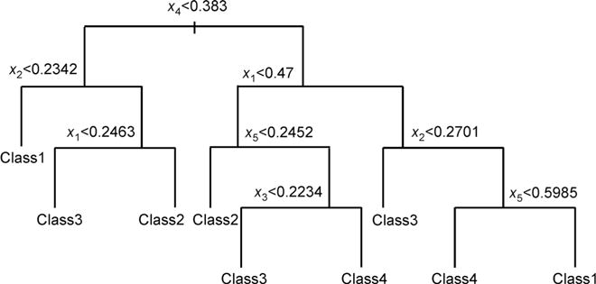
Noises are added by assigning data point in each terminal node the denoted class with probability 0.9 and any other class with probability 0.1/3.

We plot the classification error rates of all the methods with a range of training sample sizes in Figures 6–8. Unlike what was observed in the regression cases, the feature elimination Random Forests (feRF) almost consistently performed worse than the other methods. The variable importance-weighted Random Forests (viRF) and the enriched Random Forests (eRF, marginal q-value weighted) both achieved the lowest prediction error rates in most cases, while viRF was the single best classifier in the rest. It is worth noting for Models 3 with tree structures, the standard Random Forests (RF), as an ensemble of trees, performed very well when the dimension is low (occasionally even slightly better than the weighted Random Forests); however, as the number of uninformative features increased, its performance declined and the improvement by adding a weight to the features became clear (Figure 8).

Figure 6.

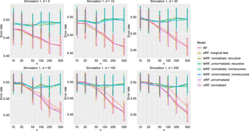
Error rate in classification simulation Model 1.

Figure 8.

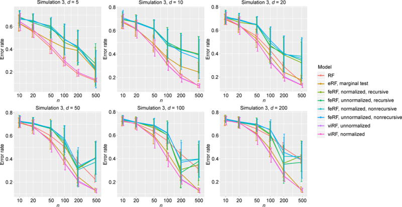
Error rate in classification simulation Model 3.

Additionally, we also considered three cases where both continuous and categorical features exist (Supplementary Figure S8) and three cases where some nuisance features are correlated with the effective features. The observations were similar to what we got on Models 1–3 (Supplementary Figures S9–S14).

In order to get more insights about these different performances, we investigated the strength of individual trees and the correlation between trees [2] for each method (Supplementary Figures S15–S23). Generally, Random Forests achieves a small correlation between trees while maintaining individual tree’s strength at the same time to give accurate classification [2]. We note that compared to the standard RF, the weighted ones (viRF and eRF) would have both increased strengths and correlations; and since their effect in strength improvement was greater than that in correlation deterioration, the overall performance was boosted. However, for feRF, the same increment in single-tree strength often brought much larger sacrifice to the correlation side, which resulted in worse performance overall.

Cancer (subtype) classification

We then assessed the performance of these methods for cancer/normal and cancer subtype classification. We considered three data sets (Table 2) with various sample sizes and input types.

Table 2.

Classification data sets summary.

Data set	Main task	Sample size	Number of features
Arcene [15]	Distinguish ovarian and prostate cancer vs. normal using mass-spectrometric data	Class 1 (cancer): 112 Class 2 (normal): 88	10,000
Pomeroy [16]	Distinguish central neural system embryonal tumor subtypes using gene expression data	Class 1: 10 Class 2: 10 Class 3: 10 Class 4: 4 Class 5: 8	5,597
Singh [17]	Distinguish prostate cancer vs. normal using gene expression data	Class 1 (cancer): 52 Class 2 (normal): 50	6,033

We performed 5-fold cross validation for 20 rounds and report the average prediction errors in Table 3. In all these three data sets, viRF performed the best. ERF (marginal test q-value weighted) also achieved better performance than the standard RF. However, similar to what we observed in the simulations, feRF performed poorly, even worse than the standard RF.

Table 3.

Cross validation error rate in cancer (subtype) classification analysis (in parentheses are standard deviations).

Data set	Arcene Overall [Class 1, Class 2]	Pomeroy Overall [Class 1, Class 2, Class 3, Class 4, Class 5]	Singh Overall [Class 1, Class 2]
viRF, normalized	0.168 (0.025) [0.078 (0.013), 0.089 (0.014)]	0.261 (0.048) [0.021 (0.017), 0.025 (0.005), 0.012 (0.014), 0.063 (0.024), 0.139 (0.030)]	0.057 (0.008) [0.013 (0.005), 0.044 (0.006)]
viRF, unnormalized	0.175 (0.028) [0.082 (0.017), 0.093 (0.015)]	0.255 (0.048) [0.026 (0.019), 0.024 (0.008), 0.014 (0.016), 0.061 (0.025), 0.130 (0.032)]	0.082 (0.011) [0.032 (0.011), 0.05 (0.004)]
eRF, marginal test	0.178 (0.017) [0.080 (0.011), 0.098 (0.013)]	0.276 (0.051) [0.029 (0.021), 0.031 (0.017), 0.013 (0.014), 0.054 (0.024), 0.150 (0.023)]	0.063 (0.011) [0.016 (0.008), 0.047 (0.006)]
feRF, normalized, recursive	0.195 (0.033) [0.100 (0.022), 0.096 (0.017)]	0.345 (0.094) [0.067 (0.035), 0.058 (0.033), 0.038 (0.029), 0.058 (0.024), 0.124 (0.033)]	0.111 (0.024) [0.054 (0.020), 0.057 (0.011)]
feRF,unnormalized, recursive	0.211 (0.027) [0.101 (0.019), 0.110 (0.017)]	0.395 (0.102) [0.073 (0.037), 0.065 (0.046), 0.056 (0.035), 0.064 (0.019), 0.137 (0.037)]	0.106 (0.024) [0.050 (0.018), 0.056 (0.016)]
feRF, normalized, nonrecursive	0.203 (0.026) [0.103 (0.015), 0.101 (0.018)]	0.339 (0.090) [0.054 (0.042), 0.058 (0.036), 0.031 (0.030), 0.064 (0.027), 0.132 (0.037)]	0.114 (0.024) [0.060 (0.014), 0.054 (0.017)]
feRF,unnormalized, nonrecursive	0.213 (0.022) [0.103 (0.016), 0.110 (0.015)]	0.319 (0.075) [0.050 (0.033), 0.044 (0.025), 0.032 (0.032), 0.061 (0.021), 0.132 (0.031)]	0.102 (0.022) [0.046 (0.016), 0.056 (0.015)]
RF	0.180 (0.022) [0.082 (0.010), 0.099 (0.015)]	0.273 (0.043) [0.015 (0.014), 0.026 (0.007), 0.008 (0.012), 0.070 (0.020), 0.152 (0.026)]	0.091 (0.011) [0.027 (0.008), 0.064 (0.006)]

The smallest overall error rates achieved for each data set is highlighted in bold.

DISCUSSION

We have proposed a variable importance-weighted Random Forests (viRF) that utilizes the variable importance scores obtained from a standard Random Forests to sample features in a weighted Random Forests. This enables the final model to rely more on informative features, hence can better deal with the growing noises as dimension increases than standard Random Forests.

Unlike the feature elimination Random Forests that removes features with small importance scores entirely, our strategy allows features with weaker information to be considered in the final model, thus it is more flexible and less prone to the inaccuracies that might occur in feature evaluation and selection steps. Especially when interactions exist between features (Simulation Model 3 and real biological data), the weighted feature sampling method is more able to capture interactions from features that might be less important marginally, and has superior performance. Besides, by avoiding the internal cross-validation that is required by feature elimination Random Forests to determine the optimal number of features, the computational burden for the weighted Random Forests is greatly reduced.

In addition, we extended a previous idea (enriched Random Forests) for continuous-feature, two-class classification problem to more general cases by utilizing the corresponding marginal test q-values to guide the random feature selection. Though theoretically such marginal tests may not provide an ideal evaluation of the features’ informativeness, in our real data analyses sometimes it presented promising results as well.

In summary, sampling features according to their informativeness in the random feature selection step could further enhance Random Forests’ performance, in both regression and classification. Since variable importance score estimated by Random Forests as the increased MSE/error rate when a feature is random permuted, provides a reliable measurement of the feature’s relevance to the outcome, we consider it a useful weight to be assigned for features. In our R implementation of the weighted Random Forests, we set default weight as the variable importance score; we also give users an option to specify other weights to use.

MATERIALS AND METHODS

Random Forests and variable importance score

Random Forests is an ensemble of classification and regression trees (CART) [2]. Each tree is grown on a bootstrapped sample from the original data set. At each node, m out of p total features are randomly selected (random feature selection) and the best split is chosen from them. The constructed trees vote for the most popular class (classification) or the mean predicted value (regression). For Random Forests classifier, an upper bound of its generalization error can be derived in terms of strength of individual trees and correlation between them [2]:

$$\mathit{PE}\ast \le \frac{\overline{\rho }\left(1-s^2\right)}{s^2},$$

where PE* is the generalization error, $\overline{\rho }$ is the average pairwise correlation between trees and s is the average single tree strength, defined as follows.

$$PE\ast =P_{\mathit{X},Y}\left(P_{\Theta }\left(h\left(\mathit{X},\Theta \right)=Y\right)-\underset{j\ne Y}{max}{P}_{\Theta }\left(h\left(\mathit{X},\Theta \right)=j\right)<0\right),$$

$$s=E_{\mathit{X},Y}\left[P_{\Theta }\left(h\left(\mathit{X},\Theta \right)=Y\right)-\underset{j\ne Y}{max}{P}_{\Theta }\left(h\left(\mathit{X},\Theta \right)=j\right)\right],$$

$$\overline{\rho }=E_{\Theta }{{ }_{,}}_{{\Theta }^{\prime }}\left[\mathit{cor}\left(I\left(h\left(\mathit{X},\Theta \right)=Y\right)-I\left(h\left(\mathit{X},\Theta \right)=\widehat{j}\left(\mathit{X},Y\right)\right),I\left(h\left(\mathit{X},{\Theta }^{\prime }\right)=Y\right)-I\left(h\left(\mathit{X},{\Theta }^{\prime }\right)=\widehat{j}\left(\mathit{X},Y\right)\right)\right)\right],$$

where X, Y are the features and true class, Θ and h(X,Θ) represent a tree and its predicted class of X, and $\widehat{j}\left(\mathit{X},Y\right)=\arg \underset{j\ne Y}{max}{P}_{\Theta }\left(h\left(\mathit{X},\Theta \right)=j\right)$.

Random Forests can also generate a variable importance score for each feature, which is evaluated as the increased classification error rate or regression MSE (measured on out-of-bag samples, i.e., samples not used to grow a tree) when a feature is randomly permuted [11]. Intuitively, permutation of an informative feature will lead to large increment in classification error rate or regression MSE while permutation of a non-informative feature will not influence the model’s performance much. A slightly modified version of variable importance score takes uncertainty of the mean increased error rate/MSE (across trees) into account by normalizing the value with the standard deviation. We considered both the unnormalized and normalized variable importance scores in our analyses, and the results did not suggest major performance difference.

Variable importance-weighted Random Forests

We propose a two-stage variable importance-weighted Random Forests (viRF) method. For the first stage, we run a standard Random Forests and obtain a variable importance score for each feature w_i, i=1, 2, …, d. Considering that it is possible for some w_i to be zero or negative, we transform these importance scores as follows:

$${\stackrel{\sim }{w}}_i=\{\begin{array}{cc}\frac{1}{d}+\frac{w_i}{\underset{j}{max}{w}_j},& \text{if}\underset{j}{max}{w}_j>0\\ \frac{1}{d},& \text{otherwise}\end{array}.$$

In the second stage, we construct another Random Forests. However, instead of sampling m features with equal probability for each feature in the random feature selection step, we sample m features with probability proportional to ${\stackrel{\sim }{w}}_i$, i=1, 2, …, d. The best split is chosen from these m features.

Other methods

Besides Random Forests’ variable importance score, we also consider a marginal testing approach to assessing the importance of a feature and perform the weighted feature sampling using the q-values of t-test (continuous-feature, two-class classification), ANOVA (continuous-feature, multiple-class classification), Chi-squared test (categorical-feature classification) or linear regression F-test (regression), following the idea of Ref. [7].

We compare the weighted Random Forests with feature elimination Random Forests [8–10]. At each iteration r% (we used r = 30 here) of the features with the least importance scores are removed and a Random Forests is constructed using the remaining ones. The number of features used in the final model is determined by cross validation. We consider both recursive (variable importance scores are updated at each iteration) and nonrecursive (variable importance scores are calculated only once at the first iteration) approaches for feature elimination, and the results did not suggest an obvious difference.

Data sets

We downloaded the CCLE data set from https://portals.broadinstitute.org/ccle/home. To reduce computational cost we kept 10,000 genes with the largest expression coefficients of variations in our analyses. We downloaded the classification data sets from http://archive.ics.uci.edu/ml/datasets/Arcene, http://stat.ethz.ch/%7Edettling/bagboost.html and http://stat.ethz.ch/%7Edettling/bagboost.html. All features included in the original data sets were used.

Figure 7.

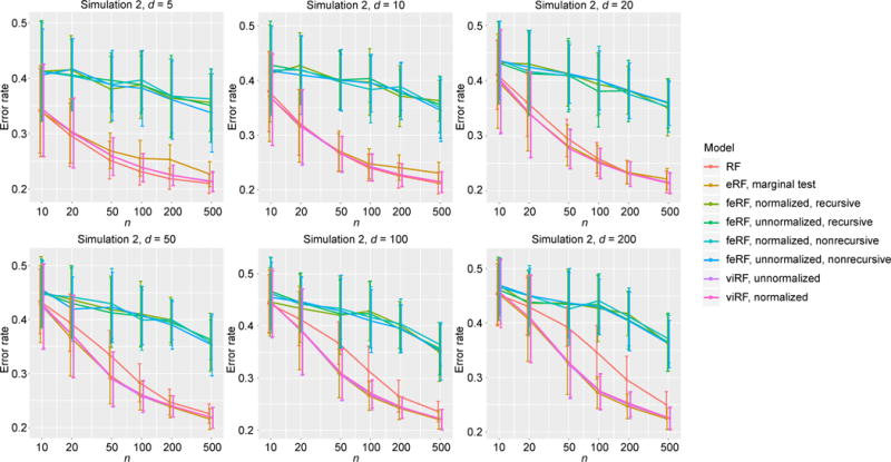
Error rate in classification simulation Model 2.

ABBREVIATIONS

RF

Random Forests

viRF

variable importance-weighted Random Forests

eRF

enriched Random Forests

feRF

feature elimiation Random Forests

References

- 1.Hanahan D, Weinberg RA. Hallmarks of cancer: the next generation. Cell. 2011;144:646–674. doi: 10.1016/j.cell.2011.02.013. [DOI] [PubMed] [Google Scholar]
- 2.Breiman L. Random forests. Mach Learn. 2001;45:5–32. [Google Scholar]
- 3.Palmer DS, O’Boyle NM, Glen RC, Mitchell JB. Random forest models to predict aqueous solubility. J Chem Inf Model. 2007;47:150–158. doi: 10.1021/ci060164k. [DOI] [PubMed] [Google Scholar]
- 4.Jiang P, Wu H, Wang W, Ma W, Sun X, Lu Z. MiPred: classification of real and pseudo microRNA precursors using random forest prediction model with combined features. Nucleic Acids Res. 2007;35:W339–W344. doi: 10.1093/nar/gkm368. [DOI] [PMC free article] [PubMed] [Google Scholar]
- 5.Lee JW, Lee JB, Park M, Song SH. An extensive comparison of recent classification tools applied to microarray data. Comput Stat Data Anal. 2005;48:869–885. doi: 10.1016/j.csda.2004.03.017. [DOI] [Google Scholar]
- 6.Goldstein BA, Polley EC, Briggs FB. Random forests for genetic association studies. Stat Appl Genet Mol Biol. 2011;10:32. doi: 10.2202/1544-6115.1691. [DOI] [PMC free article] [PubMed] [Google Scholar]
- 7.Amaratunga D, Cabrera J, Lee YS. Enriched random forests. Bioinformatics. 2008;24:2010–2014. doi: 10.1093/bioinformatics/btn356. [DOI] [PubMed] [Google Scholar]
- 8.Granitto PM, Furlanello C, Biasioli F, Gasperi F. Recursive feature elimination with random forest for PTR-MS analysis of agroindustrial products. Chemometr Intell Lab. 2006;83:83–90. [Google Scholar]
- 9.Svetnik V, Liaw A, Tong C, Wang T. Application of Breiman’s random forest to modeling structure-activity relationships of pharmaceutical molecules. Lect Notes Comput Sci. 2004;3077:334–343. [Google Scholar]
- 10.Díaz-Uriarte R, de Andrés SA. Gene selection and classification of microarray data using random forest. BMC Bioinformatics. 2006;7:3. doi: 10.1186/1471-2105-7-3. [DOI] [PMC free article] [PubMed] [Google Scholar]
- 11.Breiman L. Statistical modeling: the two cultures. Stat Sci. 2001;16:199–231. [Google Scholar]
- 12.Amaratunga D, Cabrera J. A conditional t suite of tests for identifying differentially expressed genes in a DNA microarray experiment with little replication. Stat Biopharm Res. 2009;1:26–38. [Google Scholar]
- 13.Biau G. Analysis of a random forests model. J Mach Learn Res. 2012;13:1063–1095. [Google Scholar]
- 14.Barretina J, Caponigro G, Stransky N, Venkatesan K, Margolin AA, Kim S, Wilson CJ, Lehár J, Kryukov GV, Sonkin D, et al. The cancer cell line encyclopedia enables predictive modelling of anticancer drug sensitivity. Nature. 2012;483:603–607. doi: 10.1038/nature11003. [DOI] [PMC free article] [PubMed] [Google Scholar]
- 15.Guyon I, Gunn S, Ben-Hur A, Dror G. Result Analysis of The Nips 2003 Feature Selection Challenge. Proceeding NIPS’04 Proceedings of the 17th International Conference on Neural Information Processing Systems. 2004:545–552. [Google Scholar]
- 16.Pomeroy SL, Tamayo P, Gaasenbeek M, Sturla LM, Angelo M, McLaughlin ME, Kim JY, Goumnerova LC, Black PM, Lau C, et al. Prediction of central nervous system embryonal tumour outcome based on gene expression. Nature. 2002;415:436–442. doi: 10.1038/415436a. [DOI] [PubMed] [Google Scholar]
- 17.Singh D, Febbo PG, Ross K, Jackson DG, Manola J, Ladd C, Tamayo P, Renshaw AA, D’Amico AV, Richie JP, et al. Gene expression correlates of clinical prostate cancer behavior. Cancer Cell. 2002;1:203–209. doi: 10.1016/s1535-6108(02)00030-2. [DOI] [PubMed] [Google Scholar]
Associated Data
This section collects any data citations, data availability statements, or supplementary materials included in this article.