Learning Optimal Personalized Treatment Rules in Consideration of Benefit and Risk: with an Application to Treating Type 2 Diabetes Patients with Insulin Therapies

Abstract

Individualized medical decision making is often complex due to patient treatment response heterogeneity. Pharmacotherapy may exhibit distinct efficacy and safety profiles for different patient populations. An “optimal” treatment that maximizes clinical benefit for a patient may also lead to concern of safety due to a high risk of adverse events. Thus, to guide individualized clinical decision making and deliver optimal tailored treatments, maximizing clinical benefit should be considered in the context of controlling for potential risk. In this work, we propose two approaches to identify personalized optimal treatment strategy that maximizes clinical benefit under a constraint on the average risk. We derive the theoretical optimal treatment rule under the risk constraint and draw an analogy to the Neyman-Pearson lemma to prove the theorem. We present algorithms that can be easily implemented by any off-the-shelf quadratic programming package. We conduct extensive simulation studies to show satisfactory risk control when maximizing the clinical benefit. Lastly, we apply our method to a randomized trial of type 2 diabetes patients to guide optimal utilization of the first line insulin treatments based on individual patient characteristics while controlling for the rate of hypoglycemia events. We identify baseline glycated hemoglobin level, body mass index, and fasting blood glucose as three key factors among 18 biomarkers to differentiate treatment assignments, and demonstrate a successful control of the risk of hypoglycemia in both the training and testing data set.

1 Introduction

Treatment of chronic diseases such as diabetes mellitus is often multifaceted. While maximizing clinical benefit or efficacy is the primary goal, complications and risks related to safety need to be taken into account. For example, the goal of treating patients with type 2 diabetes mellitus is to achieve a glycated hemoglobin (A1C) level of less than or equal to 7%, the level recommended by the American Diabetes Association and the European Association for the Study of Diabetes (Inzucchi et al., 2012). To attain this goal of fast and flexible control of blood glucose levels, oral hypoglycemic agents or insulin therapies are usually administered by clinicians. However, hypoglycemic events are common adverse events which may have s significant negative impact on patients. It is associated with adverse short-term and long-term outcomes, such as increased mortality, seizures, and coma. In addition, fear of hypoglycemia can lead to medication noncompliance and failure to achieve glycemic control (Cryer et al., 2003). While the progressive nature of the disease requires an escalating sequence of medications or dose of insulin, the risk of hypoglycemia and other adverse events may increase with the intensified treatment (Cryer, 2002). Hence, when choosing an optimal treatment regimen for a patient, it is necessary to consider both maximizing clinical benefit (glycemic control) and minimizing risk (hypoglycemia) at the same time.

Due to patient's differential response to a treatment, characterization of individual response heterogeneity has been a critical component of clinical decision making. Recent literature on personalized medicine has flourished with methods on using clinical and biological markers to guide the development of tailored therapies (Su et al., 2009; Lipkovich et al., 2011; Cai et al., 2011; Foster et al., 2011; Zhao et al., 2012). Several work focuses on identifying a target subgroup of subjects who are expected to gain substantial benefit from a given treatment, i.e., the right subpopulation for a given treatment (e.g., Foster et al., 2011). Some recent development aims for identifying the optimal treatment for a given subject (Qian and Murphy, 2011; Zhao et al., 2012). In particular, to estimate the optimal treatment for a patient, machine learning methods such as outcome weighted learning (Zhao et al., 2012; Liu et al., 2014) and alternatives building on double robust estimation in a semiparametric modeling framework (Zhang et al., 2012) are proposed.

The above referenced work on estimating optimal treatment strategy targets one side of clinical decision making – the clinical benefit and efficacy, but they ignore the potential safety and risk due to the “optimal” and potentially aggressive treatments. The important issue of controlling risk while maximizing benefit has long been recognized in the clinical community where safety concerns for medications often arise, since the most efficacious medication for a patient or a subpopulation may also lead to a higher risk. For example, the recent controversy regarding the safety of thiazolidinediones for treating diabetes led the new guidance issued by the Food and Drug Administration on the need to evaluate the cardiovascular risk of diabetes medications (http://www.fda.gov/downloads/Drugs/GuidanceComplianceRegulatoryInformation/Guidances/ucm071627.pdf). This new guideline calls for attention to adverse events to make accurate conclusions about the efficacy and safety of the medication. In addition, for chronic diseases such as diabetes, the long duration of treatment may expose patients to higher risk of adverse events such as hypoclycemia (Cryer et al., 2003).

Similar to the phenomenon of the heterogeneous treatment effect measured by the efficacy outcome, patients may exhibit heterogeneity in their risk profiles depending on the subject-specific characteristics. For example, Sinclair et al. (2015) reported that the risk of hypoglycemic events is higher among elder individuals. As another example, it is well-known that the relative abundance of drug-metabolizing enzymes such as cytochrome P450 (CYP450) varies from person to person, and genetic polymorphisms associated with CYP450 have been identified (Belle and Singh, 2008). Therefore, patients' adverse reactions to the same drug dosage can show between-subject heterogeneity. In addition, the efficacy outcome and safety or toxicity outcome for an individual is correlated. Increasing a subject's dosage of a medication leads to an increase in the efficacy, but may at the same time increase the risk of adverse events. Thus, in the context of identifying optimal individualized treatment rules, the goal of maximizing efficacy outcome (reward function) needs to be considered in conjunction with controlling for the risk.

An existing body of literature has considered both efficacy and safety outcomes for personalized medicine through joint modeling of the two outcomes (Houede et al., 2010; Thall et al., 2008; Thall, 2012; Lee et al., 2015). These Bayesian approaches construct a utility function or posterior criterion based on bivariate models of the efficacy and safety outcomes, and estimate an optimal dosing strategy to maximize the utility function or criterion. Subject-specific covariates are introduced to the bivariate model to estimate personalized optimal dosing strategy. Other authors propose to handle multiple outcomes while maximizing clinical benefit through a conditional regression as in Q-learning. See for example, Lizotte et al. (2012); Laber et al. (2014), and (Kosorok and Moodie, 2015, Chapter 15). Solutions were obtained by grid search or iterative methods, and no general theorem was given for a unified optimal solution. Another related work (Kosorok and Moodie, 2015, Chapter 14) proposed outcome weighted learning with a rejection option to reserve the selection of treatment and leave the actual assignment open to other considerations (including risk outcomes). Luedtke et al. (2016) considered to restrict treatment options instead of a risk outcome.

In contrast to the above existing approaches, here we aim to estimate the optimal personalized treatment rule to maximize the clinical benefit while directly impose a constraint such that the average risk under the optimal treatment assignment is lower than a pre-determined, and clinically meaningful threshold. Our approach does not require joint modeling of the efficacy and safety outcome. In addition, by directly controlling the risk while maximizing the efficacy, there is no need to examine the trade-off between the benefit and risk to form a composite outcome or utility function, as done in the benefit-risk analysis (Guo et al., 2010) or as required in some existing work (e.g., Houede et al., 2010). How to weight benefit and risk in a manner that addresses the complexity of the clinical contexts in which a medical decision is made is a separate issue that deserves attention in its own right (Moore et al., 2008). In our approach, the problem of how to compare dissimilar outcomes is avoided.

We translate the scientific goal of maximizing efficacy while controlling for the risk to a constrained optimization problem, where the resulting optimal rule is expected to maximize the clinical reward function and satisfy the risk constraint. We propose two approaches to solve the risk-constrained learning: one based on regression model with an additional constraint placed to bound the average risk (model-based benefit-risk learning, BR-M), and the other based on outcome weighted learning (benefit-risk O-learning, BR-O). For the latter, the zero-one loss in the risk constraint is approximated by a shifted ramp loss (Huang et al., 2014) instead of the usual hinge loss to allow more precise control of the risk bound. The difference of convex functions algorithm (DC algorithm, Tao and An (1998)) is applied to solve the optimization problem. We derive the theoretical optimal treatment rule under the risk constraint and show a natural connection with finding the optimal rejection region while controlling for the type I error rate as given by the familiar Neyman-Pearson lemma. We perform extensive simulation studies to examine the performance and stability of both algorithms and compare with utility function based methods. Lastly, we apply our approach to the real world motivating study to develop personalized treatment rules to guide the administration of the first line insulin treatment based on individual patient characteristics while restricting the rate of hypoglycemia events.

2 DURABLE Study: A Type 2 Diabetes Randomized Clinical Trial

Type 2 diabetes mellitus (T2DM) is a progressive disease, and the current treatment strategy is one of gradual regimen intensification. When lifestyle intervention and oral anti-diabetic agents fail to achieve adequate glycemic control, insulin treatments are often appropriate next steps. There are a variety of insulin initiation options, such as adding basal insulin or starting with twice-daily premixed insulin. To compare the efficacy, safety, and durability of two common starter insulin regimens, a randomized control clinical trial, DURABLE, was conducted to compare once-daily basal insulin glargine versus twice-daily insulin lispro mix 75/25 (Fahrbach et al., 2008). This study enrolled 2,091 patients from 242 centers in 11 countries (Argentina, Australia, Brazil, Canada, Greece, Hungary, India, the Netherlands, Romania, Spain, and the U.S.) between December 2005 and July 2007. The trial was designed with a 6-month initiation phase to compare safety and efficacy, and a subsequent 24-month maintenance phase to compare durability. The last patient visit of this trial occurred in December 2009. Because the patients had to be re-consented for the maintenance phase, the second phase was not a randomized trial any more. Therefore, we focus on the data from the first 6-month initiation phase, which consisted of 965 patients on lispro mix and 980 patients on insulin glargine.

While reducing A1C is an important efficacy goal, controlling hypoglycemia is also particularly crucial for optimizing insulin treatment regimen and patient care management. Over-medication with insulin, delays in mealtimes, or insufficient carbohydrate intake to match insulin dose are some common causes of hypoglycemia. The Diabetes Complications and Controls Trial (DCCT) found that intensive therapy for type 1 diabetes patients caused a 3-fold increase in hypoglycemic event rates compared with less aggressive treatment strategy (Control et al., 1997). Similarly, tight glycemic control in type 2 diabetes led to a significant increase in the incidence of hypoglycemia in the UK Prospective Diabetes Study (UKPDS) (Group et al., 1998). Hypoglycemia is a major limiting factor in the management of type 1 and type 2 diabetes. Patients having hypoglycemic events have symptoms ranging from hunger, sweating, to severe cases such as seizure, coma, and even death. Hypoglycemia management also relates to significant health care utilization. The mean costs for hypoglycemia visits were $17,564 for an inpatient admission, $1,387 for an emergency room visit, and $394 for an outpatient visit (Quilliam et al., 2011). As pointed out by Fidler et al. (2011), if we can successfully avoid the hypoglycemic events, glycemia targets would be much easier to achieve. Therefore, it is important to have a treatment algorithm to maximize patients benefit from insulin treatment while controlling for the risk of hypoglycemia.

Our primary efficacy measure (benefit outcome) was A1C at the study end point, and the safety measure (risk outcome) was daily hypoglycemic event rate. The study enrolled patients with baseline A1C > 7% with a median of 8.8%. The duration of diabetes at baseline ranged from 0.3 to 39 years with a median of 8 years. Our preliminary data analysis indicated that patients' responses to the treatments were heterogeneous. For example, for patients with baseline A1C > 8.8% versus ≤ 8.8%, their A1C reductions were 2.44 versus 1.08 (p-value < 0.01), and daily hypoglycemic rates were 0.061 versus 0.078 (p-value < 0.01); and for patients with baseline duration of diabetes > 8 years versus ≤ 8 years, their A1C reductions were 1.752 versus 1.746 (p-value = 0.82), and daily hypoglycemia rates were 0.082 versus 0.058 (p-value < 0.01). These pooled analyses show that the efficacy and safety endpoints are associated with some covariates but whether these covariates could further interact with the treatment assignment is largely unknown. Hence, it is important to understand the underlying heterogeneity of treatment responses for both benefit and risk outcomes so as to derive the optimal personalized treatment rules to maximize the A1c reduction while controlling for the risk of hypoglycemia.

3 Personalized Treatment Rules Maximizing Benefit While Controlling for Risk

3.1 Statistical framework

Let Y denote the benefit outcome and R denote the risk outcome. Thus, a large Y and small R is desirable. Consider a dichotomous treatment option denoted by A ∈ {−1, 1}. Let X denote subject-specific feature variables. A treatment rule is then a map from X to the treatment option domain. For any given treatment rule, say 𝒟, the expected benefit and risk are E^𝒟[Y] and E^𝒟[R], respectively, where E^𝒟[·] is the expectation under probability measure 𝒫^𝒟 for (Y, R, A, X) given that A = 𝒟(X). Our goal is to estimate a personalized treatment rule that maximizes the expected benefit while controlling the overall expected risk to be below a given threshold.

Specifically, we aim to find an optimal treatment rule, denoted by 𝒟*, such that 𝒟* solves

$$\{\begin{array}{cc}{max}_{\mathcal{D}}& E^{\mathcal{D}}(Y),\\ \text{subject to}& E^{\mathcal{D}}(R)\le \tau ,\end{array}$$ (3.1)

where τ is a pre-specified value denoting the maximal tolerance of the overall risk. For example, in the DURABLE study, Y was the reduction in HbA1C at the end point, R was the rate of hypoglycemic events, and τ was chosen to be 0.065 hypoglycemic event/day (or approximately 2 hypoglycemic events/month).

Consider data collected from a randomized trial such as DURABLE, so (Y, R, A, X) follows a non-degenerate distribution 𝒫. Furthermore, we assume that the randomization probability P(A = a|X) is bounded strictly away from zero for a ∈ {−1, 1}. Under these conditions, from the Randon-Nikodym theorem, since

$$\frac{d{\mathcal{P}}^{\mathcal{D}}}{d\mathcal{P}}=\frac{I_{a=\mathcal{D}(x)}}{p(a|x)},$$

we obtain that the expected value of treatment benefit under the rule 𝒟 is

$$E^{\mathcal{D}}(Y)=\int Yd{\mathcal{P}}^{\mathcal{D}}=\int Y\frac{d{\mathcal{P}}^{\mathcal{D}}}{d\mathcal{P}}d\mathcal{P}=E\left\{\frac{I(A=\mathcal{D}(X))}{p(A|X)}Y\right\},$$

and the expected risk under the same rule is given as

$$E^{\mathcal{D}}(R)=E\left\{\frac{I(A=\mathcal{D}(X))}{p(A|X)}R\right\}.$$

Since

$$E\left\{\frac{Y}{p(A|X)}\right\}-E\left\{\frac{I(A=\mathcal{D}(X))}{p(A|X)}Y\right\}=E\left\{\frac{I(A\ne \mathcal{D}(X))}{p(A|X)}Y\right\},$$

maximizing the benefit function is equivalent to minimizing E {I(A ≠ 𝒟(X))Y/p(A|X)}. Treatment rule 𝒟(X) is usually given as the sign of a decision function, i.e., 𝒟(X) = sign(f(X)), for some function f(X). Therefore, estimating 𝒟* using randomized trial data is equivalent to solving

$$\{\begin{array}{cc}{min}_f& E\left\{\frac{I(Af(X)<0)}{p(A|X)}Y\right\},\\ \text{subject to}& E\left\{\frac{I(Af(X)\ge 0)}{p(A|X)}R\right\}\le \tau .\end{array}$$ (3.2)

As a note, E^𝒟[Y] is termed the value function associated with the rule 𝒟. Some existing work (e.g., Zhao et al., 2012) aims to maximize this value function to find the optimal treatment rule but impose no risk control, i.e., setting τ = ∞. Here f is identifiable up to a scale. To estimate the optimal rule, only the sign of f is required. To ensure identifiability of f, a constraint on the norm of f (e.g., ‖f‖ = 1) can be imposed.

3.2 Theoretical optimal treatment rule

In this section, we will derive an explicit solution for 𝒟* that solves (3.2). First, we let δ_Y(X) = E[Y|X, A = 1] − E[Y|X, A = −1] and δ_R(X) = E[R|X, A = 1] − E[R|X, A = −1]. Note that (3.2) is equivalent to

$$\begin{array}{ccc}\underset{f}{max}E\{{\delta }_Y(X)I(f(X)>0)\}& \text{subject to}& E\{{\delta }_R(X)I(f(X)>0)\}\le \alpha ,\end{array}$$

where α = τ − E {E(R|A = −1, X)}. Clearly, from the constraint, we require that α ≥ E{δ_R(X)I(δ_R(X) < 0)} since otherwise, no f exists. In other words, τ cannot be too small so that no treatment rule can induce risk below τ. Additionally, we assume X to be continuous.

To derive the optimal treatment rule, we consider two different domains of X: ℳ = {X : δ_Y(X)δ_R(X) ≤ 0} and ℳ^c. Clearly, for X ∈ ℳ, treatment options yielding higher benefit also reduce risk or treatments yielding lower benefit also increase risk; while it is the opposite for X ∈ ℳ^c. Hence, for X ∈ ℳ, we choose f*(X) = sign(δ_Y(X)) which gives the largest benefit and smallest risk.

It only remains to determine f*(X) for X ∈ ℳ^c. The objective function to be maximized becomes

$$\begin{array}{ccc}E\{{\delta }_Y(X)I(f(X)>0)|X\in {\mathcal{M}}^c\},& \text{subject to}& E\{{\delta }_R(X)I(f(X)>0)|X\in {\mathcal{M}}^c\}\le {\alpha }^{\ast }\end{array},$$

Where

$${\alpha }^{\ast }=\frac{\alpha -E\{{\delta }_R(X)I({\delta }_Y(X)>0,X\in \mathcal{M})\}}{P(X\in {\mathcal{M}}^c)}=\frac{\alpha -E\{{\delta }_R(X)I({\delta }_Y(X)>0,{\delta }_R(X)\le 0)\}}{1-P({\delta }_Y(X)>0,{\delta }_R(X)\le 0)-P({\delta }_Y(X)\le 0,{\delta }_R(X)>0)}.$$

The optimal rule is given in the following theorem.

Theorem 1 The optimal treatment rule is 𝒟*(X) = sign(f*(X)), where

$${\mathcal{D}}^{\ast }(X)=\mathit{\text{sign}}({\delta }_Y(X)-{\lambda }^{\ast }{\delta }_R(X)),$$

where λ* = 0 if $E[{\delta }_R^{+}(X)|X\in {\mathcal{M}}^c]\le {\alpha }^{\ast }$; otherwise, λ* solves equation

$$E[{\delta }_R(X)I\{{\delta }_R(X)>0,{\delta }_Y(X)/{\delta }_R(X)>\lambda \}|X\in {\mathcal{M}}^c]+E[{\delta }_R(X)I\{{\delta }_R(X)<0,{\delta }_Y(X)/{\delta }_R(X)<\lambda \}|X\in {\mathcal{M}}^c]={\alpha }^{\ast }.$$

The proof of Theorem 1 is given in Appendix A.

Remark 1. The proof of Theorem 1 shows that estimating the optimal treatment rule is analogous to finding the optimal rejection region at a given type I error rate as in the Neyman-Pearson lemma, which aims to maximize the power under an alternative hypothesis while controlling the type I error under the null. Therefore, if X is not continuous, there may not exist an exact solution λ* to satisfy the last equation. In this case, similar to the Neyman-Pearson lemma, we propose to adopt a probability distribution to assign the optimal treatment. Analogous to the fact that the optimal test in Neyman-Pearson lemma is the likelihood ratio test, our optimal treatment rule depends on the benefit-risk ratio, δ_Y(X)/δ_R(X).

Remark 2. When there is no treatment heterogeneity on safety outcomes in the population, Theorem 1 still applies with δ_R(X) = c, which is a special case of our general scenario allowing δ_R(·) to depend on X.

4 Estimation of the Optimal Treatment Rules

In this section, we propose two learning algorithms to estimate the optimal treatment rules using data collected from a randomized trial: regression-based learning and O-learning (abbreviated for outcome weighted learning) in the benefit-risk framework. In the subsequent development, we assume that data consist of (Y_i, R_i, A_i, X_i) for i = 1, …, n.

4.1 Regression-model-based learning algorithm (BR-M learning)

Our first algorithm is based on explicitly estimating the solution as given in Theorem 1. We use the empirical observations to fit regression models for Y given (A, X) and for R given (A, X), respectively. From the fitted model, we can estimate δ_Y(X) and δ_R(X) by δ̂_Y(X) and δ̂_R(X). Let ℳ̂ = {x : δ̂_Y(x)δ̂_R(x) ≤ 0} and

$${\widehat{\alpha }}^{\ast }=\frac{\tau -{\overline{R}}_1-n^{-1}{\sum }_{i=1}^n[{\widehat{\delta }}_R(X_i)I({\widehat{\delta }}_Y(X_i)>0,X_i\in \widehat{\mathcal{M}})]}{n^{-1}{\sum }_{i=1}^{n}I(X_i\in {\widehat{\mathcal{M}}}^c)},$$

where R̄₁ is the average risk outcome in subjects with A = 1. Theorem 1 implies that the optimal treatment rule can be estimated by D̂(X) = sign(f̂(X)), where

$$\widehat{f}(X)=\{\begin{array}{cc}\text{sign}({\widehat{\delta }}_Y(X)),& X\in \widehat{\mathcal{M}}\\ \text{sign}({\widehat{\delta }}_Y(X)-\widehat{\lambda }{\widehat{\delta }}_R(X)),& X\in {\widehat{\mathcal{M}}}^c\end{array}$$

with λ̂ = 0 if

$$\frac{{\sum }_{i=1}^n{\widehat{\delta }}_R^{+}(X_i)I(X_i\in {\widehat{\mathcal{M}}}^c)}{{\sum }_{i=1}^{n}I(X_i\in {\widehat{\mathcal{M}}}^c)}\le {\alpha }^{\ast },$$

and otherwise, λ̂ is the solution to

$$\begin{gathered} \frac{{\sum }_{i=1}^n{\widehat{\delta }}_R(X_i)I(X_i\in {\widehat{\mathcal{M}}}^c,{\widehat{\delta }}_R(X_i)>0,{\widehat{\delta }}_Y(X_i)/{\widehat{\delta }}_R(X_i)>\lambda )}{{\sum }_{i=1}^{n}I(X_i\in {\widehat{\mathcal{M}}}^c)} \\ +\frac{{\sum }_{i=1}^n{\widehat{\delta }}_R(X_i)I(X_i\in {\widehat{\mathcal{M}}}^c,{\widehat{\delta }}_R(X_i)<0,{\widehat{\delta }}_Y(X_i)/{\widehat{\delta }}_R(X_i)<\lambda )}{{\sum }_{i=1}^{n}I(X_i\in {\widehat{\mathcal{M}}}^c)}={\alpha }^{\ast }. \end{gathered}$$

The regression models can be fitted by linear regression with a sparse penalty when the number of covariates is large.

4.2 Outcome-weighted learning algorithm (BR-O learning)

Our second algorithm directly solves the empirical version of (3.2) using machine learning approaches. This approach is a non-trivial extension of the non-constrained O-learning where maximizing benefit without risk control is the goal. Denote p_i = p(A_i|X_i). We propose to solve the following optimization problem:

$$\{\begin{array}{cc}{min}_f& n^{-1}{\sum }_{i=1}^n\frac{Y_i}{p_i}I(A_{i}f(X_i)<0),\\ \text{subject to}& n^{-1}{\sum }_{i=1}^n\frac{R_i}{p_i}I(A_{i}f(X_i)\ge 0)\le \tau .\end{array}$$ (4.1)

However, due to the discontinuity of the indicator function corresponding to the zero-one loss, solving the above constrained optimization problem in (4.1) is an NP-hard problem (Natarajan, 1995). Thus, instead of using the zero-one loss in the optimization, we consider other types of surrogate loss functions and propose feasible algorithms to obtain solutions.

First, following Liu et al. (2014), we modify the above optimization problem to (a) reduce the variability of weights (Y_i/p_i) in the objective function, and (b) handle the situation that the weights in the objective function can be negative, especially after (a). Specifically, for (a), instead of using the original Y as outcomes, we first regress Y on X and let the residuals be the outcomes. The validity of using the residual is because

$$arg\underset{\mathcal{D}\in \mathrm{\Delta }}{max}E\left\{\frac{I(A=\mathcal{D}(X))}{p(A|X)}Y\right\}=arg\underset{\mathcal{D}\in \mathrm{\Delta }}{max}E[\frac{I(A=\mathcal{D}(X))}{p(A|X)}\{Y-m(X)\}],$$

where m(X) is any function of X. For (b), we note

$$\begin{gathered} E\left\{\frac{I(A=\mathcal{D}(X))}{p(A|X)}Y\right\} \\ +E\left\{\frac{Y^{-}}{p(A|X)}\right\} \\ =E\left\{\frac{I(A=\mathcal{D}(X))}{p(A|X)}{Y}^{+}\right\} \\ +E\left\{\frac{I(A\ne \mathcal{D}(X))}{p(A|X)}{Y}^{-}\right\} \\ =E\{\frac{I(A\cdot \text{sign}(Y)=\mathcal{D}(X))}{p(A|X)}|Y|\}. \end{gathered}$$

This suggests that the original optimization problem can be modified as follows. Define $Y_i^{\ast }=|Y_i-m(X_i)|$, $A_i^{\ast }=\text{sign}\{Y_i-m(X_i)\}{A}_i$, equation (4.1) is equivalent to

$$\{\begin{array}{cc}{min}_f& {\sum }_{i=1}^n\frac{Y_i^{\ast }}{p_i}I(A_i^{\ast }f(X_i)<0),\\ \text{subject to}& {\sum }_{i=1}^n\frac{R_i}{p_i}I(A_{i}f(X_i)\ge 0)\le n\tau .\end{array}$$ (4.2)

Since the indicator function in the objective function is discontinuous, we introduce a slack variable as the usual support vector machine, and adopt the kernel tricks to estimate f. Specifically, we let $f(X|\beta )={\beta }_0+{\sum }_{j=1}^n{\beta }_{j}K(X,X_j)$ where K(·, ·) is a reproducing kernel and introduce slack variables, ${\xi }_i\ge 1-A_i^{\ast }f(X|\beta )$, and ξ_i ≥ 0. Then, the optimization problem becomes

$$\{\begin{array}{cc}{min}_f& C{\sum }_{i=1}^n\frac{Y^{\ast }}{p_i}{\xi }_i+\frac{1}{2}{\Vert f\Vert }_{\mathcal{H}},\\ \text{subject to}& {\sum }_{i=1}^n\frac{R_i}{p_i}I(A_{i}f(X_i)\ge 0)\le n\tau ,\\ & {\xi }_i\ge 1-A_i^{\ast }\{{\beta }_0+{\sum }_{j=1}^n{\beta }_{j}K(X_i,X_j)\},{\xi }_i\ge 0\forall i.\end{array}$$ (4.3)

Here, ${\Vert f\Vert }_{\mathcal{H}}^2$ is the norm for the reproducing kernel Hilbert space which is equivalent to ${\beta }_{(0)}^T\mathbf{K}{\beta }_{(0)}$ with K being the kernel matrix and β₍₀₎ = {β₁, …, β_n}^T.

In the above optimization, the non-convex indicator function in the constraint makes computation difficult. To avoid this discontinuity, we approximate I{Af(X) ≥ 0} by the following shifted ramp loss (Huang et al., 2014, see also Figure 1):

Figure 1. Comparison of zero-one loss, hinge loss, and shifted ψ–loss*.

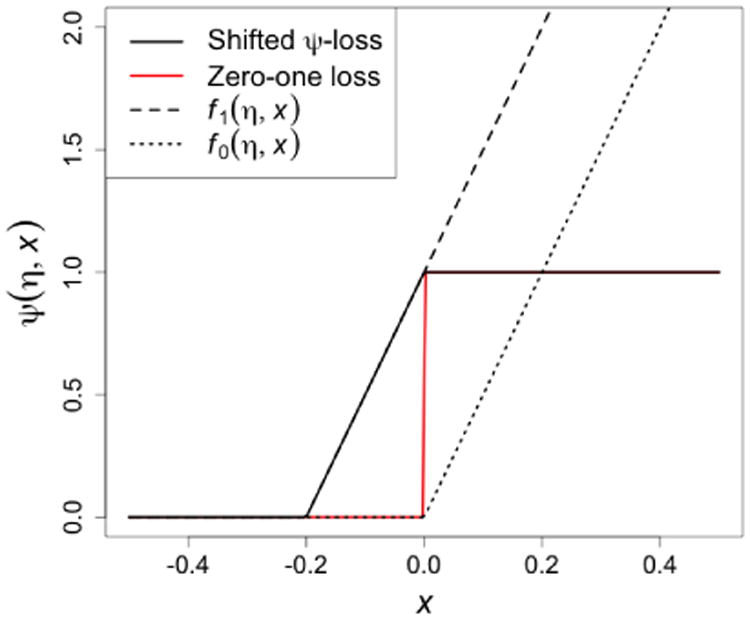
*: Shifted ψ-loss is defined as ψ(η, x) = f₁(η, x) − f₀(η, x) = η⁻¹(x + η)₊ − η⁻¹(x)₊.

$$\psi (\eta ,x)=f_1(\eta ,x)-f_0(\eta ,x)={\eta }^{-1}{(x+\eta )}_{+}-{\eta }^{-1}{(x)}_{+}.$$

As we can see that ψ(η, x) ≥ I(x ≥ 0), thus the shifted ψ-loss serves as an upper bound of the zero-one loss function. Therefore, if we can control the risk under loss function ψ(η, x), we can also control the risk under the zero-one loss. In summary, the final solution for f* solves

$$\{\begin{array}{cc}{min}_f& C{\sum }_{i=1}^n\frac{Y^{\ast }}{p_i}{\xi }_i+\frac{1}{2}{\beta }_{(0)}^T\mathbf{K}{\beta }_{(0)},\\ \text{subject to}& {\sum }_{i=1}^n\frac{R_i}{p_i}[{\eta }^{-1}{\{A_{i}f(X_i)+\eta \}}_{+}-{\eta }^{-1}{\{A_{i}f(X_i)\}}_{+}]\le n\tau ,\\ & {\xi }_i\ge 1-A_i^{\ast }\{{\beta }_0+{\sum }_{j=1}^n{\beta }_{j}K(X_i,X_j)\},{\xi }_i\ge 0\forall i.\end{array}$$ (4.4)

We present the detailed algorithm for solving the above optimization problem in the Appendix. Briefly speaking, by expressing the non-convex loss function as the difference of two convex functions, the DC algorithm (Tao and An, 1998) can be applied for optimization, and the tuning parameters are chosen by cross-validation. To stabilize optimization, all covariates will be standardized before fitting the DC algorithm.

5 Simulation Studies

We simulated 10 i.i.d. covariates, X₁, …, X₁₀, from a Uniform(0, 1) distribution. The efficacy responses Y and safety responses R were generated from two continuous distributions,

$$\begin{array}{c}Y=1-2X_1+X_2-X_3+h_Y(X,A)+{\epsilon }_Y,\\ R=2+X_1+h_R(X,A)+{\epsilon }_R,\end{array}$$

where ε_Y follows N(0, 1), ε_R follows a truncated standard normal distribution (truncated at 1), h_Y(X, A) and h_R(X, A) are the interaction terms between covariates and treatment for the efficacy and risk outcome, respectively. Here A takes two values: 1 (experimental therapy) and −1 (standard of care), and the randomization probability is 0.5. In the first simulation setting, we considered the decision rules for both risk and efficacy to be linear, that is,

$$\begin{array}{cc}{h}_Y(X,A)=2(1-X_1-X_2)A,& h_R(X,A)=(1+X_1-X_2)A.\end{array}$$

In this setting, regardless of whether all subjects are given the experimental therapy or standard treatment, the average efficacy values do not vary greatly and they are both close to 0. However, the risk of receiving the experimental therapy is much higher (3.503) as compared to the standard treatment (1.496). If ignoring the risk outcomes, the optimal treatment strategy based on the efficacy alone results in a maximal efficacy of 0.670 while the average risk reaches 2.495. Therefore, if the safety outcome above some level, say 2.0, is of great concern, this optimal treatment strategy is highly risky and not acceptable.

To illustrate how the risk constraint may affect the optimal treatment decision boundary, in Figure 2 we plot these boundaries and present the partition of optimal treatment regions. Without the risk constraint, the optimal treatment decision boundary is a linear function, X₁ + X₂ = 1, so the optimal treatment for subjects in regions A and B is the experimental therapy, TRT, because the benefit function δ_Y(X) is positive in these regions. Similarly, the optimal treatment for subjects in region C is the standard of care, SOC, because there is no gain in terms of the efficacy for TRT. However, when considering risk constraint, subjects in region B originally with TRT the as the optimal treatment should be changed to receiving SOC instead, since the benefit gain from TRT is moderate but the average risk is higher for this group as demonstrated by the contour lines of the risk differences. Subjects in region A maintain TRT as their optimal treatment taking into account of risk because the benefit is higher in this group. Likewise, subjects in region C maintain SOC as the optimal treatment since SOC shows a higher benefit and the risk is always lower than TRT. This region mimics the real world scenario where a safer medication is preferred when the efficacy is similar.

Figure 2.

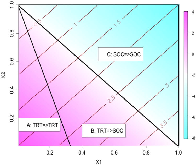
Regions of optimal treatment rules with τ = 1.75 in the first simulation setting.

For each simulated data, we applied the proposed two methods to estimate the optimal treatment rules, where we varied the risk threshold τ from 1.75 to 2.25. In the BRM learning, we estimated both δ_Y(X) and δ_R(X) using linear regression models with interactions between X and A included. We then estimated the optimal treatment rule using the expression in Section 4.1, where λ̂ was calculated using a grid search algorithm. In the BR-O learning, we chose the kernel function to be a linear kernel, i.e., K(x, x) = x^Tx. The DC algorithm was used to solve the optimization problem, where at each iteration we used an existing quadratic programming package (“ipop” in R package kernlab https://cran.r-project.org/web/packages/kernlab/kernlab.pdf) for the optimization. The tuning parameters, C and δ, for BR-O were chosen by 2-fold cross validation. The data was split into a training set and a testing set. On the training set, the optimal treatment rule was computed with the risk constraint. On the testing set, the empirical average of the efficacy outcome under the derived rule was computed and used as the criterion for the cross validation. We let C vary from 0.5 to 2 and δ between 0.01 and 0.05. To compare different methods, we independently generated a validation data set of size 20,000 and applied the estimated decision rules to the validation data in order to assess the predicted efficacy and risk on this large testing set. We also calculated the efficacy of the theoretical optimal treatment rule using Theorem 1.

The simulation results from 100 replicates for this setting are shown in Table 1. BR-M and BR-O perform similarly: with a more lenient threshold τ, the average risk increases and average efficacy also increases. Both methods control the risk to be close to the pre-specified level and the estimated optimal treatment agrees with the true optimal treatment for most subjects (proportion of agreement greater than 85%). With a smaller sample size, BR-M provides a slightly larger efficacy and a higher probability of identifying the correct optimal treatment. With increasing sample size, both methods show improved performance. The median efficacy and risk is similar to the mean. Since the true optimal treatment boundary is linear, the model-free BR-O may not greatly improve the performance as compared to the model-based BR-M.

Table 1. Estimated average risk and optimal benefit in the first simulation setting^†.

τ	Efficacy	n	Method	M-risk (sd)	M-effic (sd)	P-risk (dev)	P-effic (dev)	Accuracy
1.75	0.370	200	BR-M	1.751 (0.062)	0.338 (0.062)	1.750 (0.039)	0.337 (0.037)	93% (1.6%)
			BR-O	1.776 (0.136)	0.321 (0.125)	1.763 (0.094)	0.335 (0.085)	89% (2.5%)
		400	BR-Q	1.747 (0.041)	0.345 (0.042)	1.743 (0.028)	0.349 (0.027)	95% (1.2%)
			BR-O	1.773 (0.111)	0.331 (0.102)	1.768 (0.072)	0.344 (0.068)	90% (1.7%)
2.00	0.556	200	BR-M	2.004 (0.070)	0.525 (0.040)	2.009 (0.041)	0.530 (0.025)	92% (1.8%)
			BR-O	2.005 (0.154)	0.487 (0.091)	1.993 (0.107)	0.492 (0.066)	87% (3.1%)
		400	BR-M	2.001 (0.049)	0.535 (0.028)	1.999 (0.037)	0.535 (0.020)	95% (1.4%)
			BR-O	2.006 (0.113)	0.505 (0.067)	2.000 (0.082)	0.512 (0.049)	90% (2.2%)
2.25	0.648	200	BR-M	2.261 (0.070)	0.617 (0.019)	2.260 (0.051)	0.622 (0.012)	92% (1.9%)
			BR-O	2.216 (0.154)	0.576 (0.055)	2.225 (0.091)	0.592 (0.034)	88% (3.6%)
		400	BR-M	2.251 (0.050)	0.626 (0.015)	2.254 (0.037)	0.626 (0.011)	94% (1.3%)
			BR-O	2.242 (0.102)	0.604 (0.029)	2.236 (0.063)	0.604 (0.021)	91% (2.2%)

^†“Efficacy” is the theoretical efficacy value under the risk constraint; “M-risk” is the mean of the predicted risk in the validation data; “M-effic” is the mean of the predicted efficacy using an independent validation data set of size 20,000; “sd” is the empirical standard deviation; “P-risk” is the median of the predicted risk in the validation data; “P-effic” is the median of the predicted efficacy using an independent validation data set of size 20,000; “dev” is the median of the absolute value of the deviation from the median; “Accuracy” is the proportion of subjects whose predicted optimal treatments agree with the true optimal treatments. The numbers in the parentheses are the median absolute deviation from 100 replicates.

Next, we examined a procedure to rank variable importance using the magnitude of the coefficients of the fitted linear optimal treatment rule. In this simulation setting, the first two feature variables were equally informative (same coefficient on the optimal treatment rule) and the other variables were noise. The average estimated rank based on the absolute value of the fitted coefficient is 1.46 (sd = 0.50) for X₁ and 1.53 (sd = 0.50) for X₂, where the true rank for both variables is 1.5. The eight noise variables have an average rank of 6.50 across 100 simulations, while the true rank is also 6.5. These results suggest that using the magnitude of the coefficients of the optimal rule to determine variable importance is effective when the true optimal rule is linear.

In the second simulation setting, we considered a nonlinear efficacy and safety boundaries by letting

$$\begin{array}{c}Y=1-2X_1+X_2-X_3+h_Y(X,A)+{\epsilon }_Y,\\ R=2+X_1+h_R(X,A)+{\epsilon }_R,\end{array}$$

where ε_Y and ε_R were generated the same as in the previous setting but

$$\begin{array}{cc}{h}_Y(X,A)=8(1-X_1^2-X_2^2)A,& h_R(X,A)=(X_1+X_2-0.3)A.\end{array}$$

The covariates and treatment assignments were the same as setting 1. Figure 3 illustrates 3 regions partitioned by the nonlinear optimal treamtent boundaries. The optimal treatment for subjects in Region C is SOC due to a negative benefit function. However, the risk of treating subjects in region B with TRT is too high (δ_R(X) > 0 with large magnitude). Thus, for region B, the optimal treatment should be switched to SOC when considering risk regardless of a slightly inferior efficacy on SOC. This scenario is similar to setting 1 except that the optimal decision boundaries are nonlinear. The average risk is 2.661 and the theoretical maximal efficacy without risk constraint is 3.602.

Figure 3.

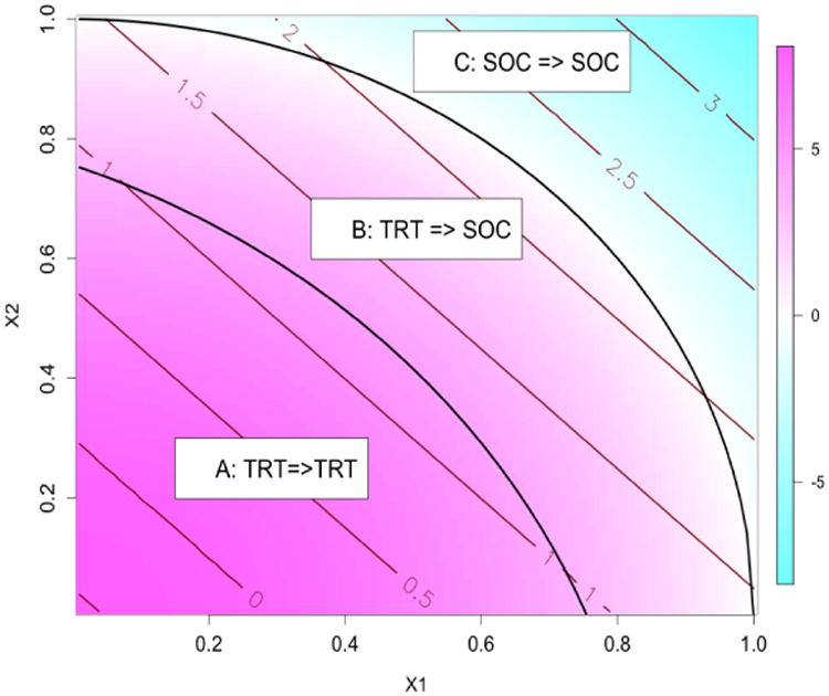
Regions of optimal treatment rules with τ = 2.0 in the second simulation setting.

The results from setting 2 are summarized in Table 2. Both methods adequately control the risk since the risk outcome is simulated from a linear model. For small sample size, BR-M has slightly higher efficacy and a smaller variability in estimating benefit function since it is model-based. The variability of BR-O is larger than BR-M, leading to some outliers and a slightly smaller mean benefit. When considering median benefit, BR-O performs as well as BR-M even for small sample size: for τ = 2.0 and n = 200, the median efficacy for BR-O and BR-M are: 1.801 and 1.834, respectively. With larger sample size, the variability of BR-O is reduced and it has a greater mean benefit (and a greater median benefit) than BR-M under all values of τ.

Table 2. Estimated average risk and optimal benefit in the second simulation setting^†.

τ	Efficacy	n	Method	M-risk (sd)	M-effic (sd)	P-risk (dev)	P-effic (dev)	Accuracy
2.0	1.843	200	BR-M	2.008 (0.051)	1.758 (0.402)	2.008 (0.030)	1.801 (0.226)	94% (2.0%)
			BR-O	2.052 (0.139)	1.737 (1.064)	2.026 (0.101)	1.834 (0.666)	88% (6.0%)
		400	BR-M	2.005 (0.037)	1.785 (0.274)	2.009 (0.027)	1.823 (0.184)	95% (1.0%)
			BR-O	2.037 (0.094)	1.858 (0.701)	2.036 (0.052)	1.944 (0.350)	91% (4.2%)
2.1	2.467	200	BR-M	2.107 (0.051)	2.363 (0.267)	2.107 (0.033)	2.399 (0.138)	93% (1.1%)
			BR-O	2.135 (0.137)	2.296 (0.689)	2.131 (0.107)	2.438 (0.455)	88% (3.9%)
		400	BR-M	2.106 (0.042)	2.380 (0.207)	2.107 (0.026)	2.402 (0.128)	94% (0.9%)
			BR-O	2.134 (0.099)	2.408 (0.488)	2.124 (0.066)	2.462 (0.299)	91% (3.2%)
2.2	2.902	200	BR-M	2.202 (0.053)	2.766 (0.197)	2.202 (0.031)	2.778 (0.109)	92% (0.9%)
			BR-O	2.221 (0.157)	2.642 (0.602)	2.221 (0.100)	2.789 (0.334)	88% (4.4%)
		400	BR-M	2.202 (0.041)	2.781 (0.146)	2.207 (0.024)	2.814 (0.082)	93% (0.4%)
			BR-O	2.232 (0.111)	2.797 (0.390)	2.230 (0.078)	2.852 (0.249)	90% (2.6%)

^†See Table 1.

In the above two simulation settings, we also estimated the optimal rules using the BR-O under a Gaussian kernel. For the Gaussian kernel, following Jaakkola et al. (1999) and Wu et al. (2010), we used a heuristic method to choose the spread parameter σ as $\sigma =1/d_m^2$, where d_m was the median pairwise Euclidean distance defined as median{‖X_i − X_j‖ : A_i ≠ A_j}. The performance was very similar to using the linear kernel with a slightly larger efficacy in the nonlinear setting. However, the computational time using the Gaussian kernel was much more intensive. Therefore, a linear kernel for BR-O may be sufficient in practice.

As a comparison, we also implemented a utility based method inspired by Thall et al. (2008). Let U(Y_i, R_i) = Y_i − βR_i denote a utility function, where β reflects the equivalent benefit loss for one unit increase in risk and is computed as the regression coefficient of Y_i on R_i using the population data. Specifically, β = 0.091 and 0.093 for the two simulation settings, respectively. Following Thall et al. (2008), we fitted a bivariate copula model to estimate the joint distribution of efficacy and risk outcome including treatment by covariate interactions, and computed the expected utility given the joint distribution for each patient. The optimal treatment was estimated as the one leading to a higher utility value. Under simulation setting 1, the mean efficacy (sd) was 0.622 (0.015) and 0.634 (0.008) for n = 200 and n = 400, respectively. The mean risk (median absolute deviation) was 2.620 (0.078) and 2.629 (0.053), respectively. The median efficacy and risk were similar to the mean. For setting 2, the mean (sd) of the efficacy was 3.521 (0.017) and 3.526 (0.012), for the two sample sizes, respectively. The corresponding mean (sd) for the risk outcome was 2.563 (0.023) and 2.558 (0.017), respectively. These results show that the utility based method captures the optimal efficacy, but does not provide control over the risk at a particular level. Thus, the higher efficacy is achieved by allowing a higher risk, where the latter may potentially be over the tolerance bound.

Next, we explored a modified utility-based method that provides more control over individual risk outcome by imposing a safety admission rule: for each individual, we examine whether the previously estimated utility-based treatment rule will lead to a risk outcome (or estimated risk outcome) exceeding the threshold τ; if so, we select the safer treatment with a lower risk regardless of the efficacy. The results under the first simulation setting show that utility-based approach with safely admission rule leads to the risk outcome being controlled well below the threshold, at the price of a lower efficacy than BR-M and BR-O. For example, for setting 1, the mean efficacy across simulations was 0.016 and the mean risk was 1.49 when τ = 2.0 and n = 200. When τ = 2.25, the mean risk and efficacy was 1.50 and 0.0164, respectively. The efficacy is close to that of the non-personalized, “one-size-fits-all” rule (treatment effect of 0.003). This may be due to that the risk constraint is imposed at the individual level for this utility-based approach, while for BR-M and BR-O the risk is controlled on average (across patients). Thus, when strictly enforcing each individual's risk to be below τ is desirable, utility-based method with a safety admission rule is preferable.

6 Application to DURABLE Trial

We applied our method to DURABLE study (Fahrbach et al., 2008) introduced in Section 2. A more detailed description of the study design was previously published (Fahrbach et al., 2008; Buse et al., 2009). A major objective of treating diabetes patients was to lower patients' blood glucose measured by A1C. Similar to the original report in Fahrbach et al. (2008), our efficacy endpoint (the benefit) was A1C change from baseline at 24 weeks (last observation carried forward [LOCF] to 24 weeks). Our safety (the risk) endpoint was measured by daily hypoglycemic event rate. We considered 18 relevant covariates measured at the baseline, including baseline A1C, fasting blood glucose, fasting insulin, adiponectin, blood pressure, 7 points self monitored blood glucose, duration of diabetes, weight, height, blood pressure, body mass index (BMI). The covariates were standardized before fitting the model and the tuning parameters for BR-O were chosen by 2-fold cross validation similar to the simulation studies.

We included randomized patients who received at least one treatment, which consisted of 965 patients on lispro mix and 980 patients on insulin glargine. Within a reasonable range, we examined different threshold values for daily hypoglecemic rates (τ = 0.063, 0.064, 0.065, 0.066, 0.067) as our safety constraint. To compare the performance of different methods and evaluate the importance of the variables in this analysis, we randomly split the full data into a training set and a testing set, so the performance can be assessed using the testing set. Among 1,945 patients, we randomly selected 300 patients as a training set, and used the rest 1,645 patients as a testing set. We applied the proposed algorithms (BR-M, BR-O) to the training set, and obtained the average efficacy and safety outcomes under the estimated optimal treatment assignments on the testing set. Furthermore, to minimize influence on the variability due to selecting training and testing set by chance, we repeated this procedure 100 times.

We show in Table 3 the average benefit and risk obtained by BR-M and BR-O under risk constraints, and compare with results obtained by O-learning without controlling for the risk (Zhao et al., 2012). We see that the average risks are reasonably controlled for both BR-M and BR-O at all constraint value of τ. BR-O produces a more conservative result in terms of a lower rate of hypoglycemia on the testing set as compared to BR-M, and thus a slightly lower average benefit. The average benefit increases as a function of threshold τ, indicating that allowing a more lenient risk control leads to gain in efficacy. The maximal benefit for the optimal treatment rules under O-learning without constraint (τ = ∞) is the highest (1.738).

Table 3.

DURABLE study analysis results. We randomly selected 300 patients as a training dataset, used the rest 1,645 patients as a testing dataset, and repeated this 100 times. The average benefit, risk and their standard deviations are shown.

Risk(τ)	Method	Risk-Training	Risk-Testing	Benefit-Training	Benefit-Testing
0.063	BR-M	0.0639(0.005)	0.0689(0.004)	1.8668(0.142)	1.7201(0.049)
	BR-O	0.0626(0.003)	0.0640(0.006)	1.7824(0.142)	1.6980(0.042)
0.064	BR-M	0.0644(0.006)	0.0690(0.004)	1.8682(0.141)	1.7209(0.050)
	BR-O	0.0632(0.003)	0.0650(0.006)	1.7905(0.135)	1.7004(0.050)
0.065	BR-M	0.0652(0.006)	0.0692(0.004)	1.8736(0.142)	1.7228(0.050)
	BR-O	0.0638(0.003)	0.0650(0.006)	1.7983(0.135)	1.7030(0.051)
0.066	BR-M	0.0657(0.006)	0.0694(0.004)	1.8780(0.146)	1.7241(0.051)
	BR-O	0.0644(0.003)	0.0655(0.006)	1.8048(0.135)	1.7021(0.046)
0.067	BR-M	0.0667(0.006)	0.0696(0.004)	1.8827(0.148)	1.7250(0.052)
	BR-O	0.0654(0.003)	0.0660(0.006)	1.8273(0.131)	1.7093(0.048)
∞	BR-M	0.0756(0.010)	0.0712(0.003)	1.9392(0.153)	1.7378(0.048)
	BR-O	0.0769(0.010)	0.0714(0.005)	1.9895(0.146)	1.7360(0.052)

Since a linear kernel was used for the BR-O algorithm, the treatment decision boundary can be expressed as a linear combination of the covariates. The standardized effects can be used to compare influences of the covariates on the decision boundary and rank the importance of covariates (absolute value of the standardized coefficient). The ranking based on covariates' average effects from 100 random splits indicates that the top 3 most important variables are, in turn, baseline fasting blood glucose, BMI and A1C. The variables with highest importance are not sensitive to the threshold of the risk constraint. The less important variables can change order in the presence and absence of risk constraint (e.g., fasting insulin and heart rate).

To determine an appropriate risk bound for the final model, we control the rate of hypoglycemic event to be below the observed incidence rate in the low risk treatment arm (insulin glargine) in DURABLE trial, an incidence rate of 0.5 per week for each patient (Buse et al., 2009, Table 2, a total of 530 incidences per week for 1,046 patients), which corresponds to 2 hypoglycemic events per month (i.e., τ = 0.065). To further illustrate an empirical method to choose the threshold, we adapt the net clinical benefit (NCB) which was proposed to weigh benefits against harms of a treatment based on the difference between expected benefit and expected harm (Lynd, 2006; Sutton et al., 2005). Specifically, the NCB at each threshold was computed as Y − 1.5R, where Y was the average efficacy obtained on the testing set using BR-O, and R was the corresponding average risk on the testing set (Table 3). The scaled association coefficient of 1.5 was obtained from the full data, similar to the method used for constructing the utility function. The increase in NCB with increasing threshold was 0.0026, 0.0029, -0.0024, and 0.0098 for τ changing from 0.063 to 0.067 at an increment of Δτ = 0.001. Thus, when τ = 0.065 the change in NCB is negative for the first time, i.e., the change in benefit does not outweigh the change in risk. This analysis further supports the choice of τ = 0.065 as the threshold.

Next, we present the estimated optimal treatment rule obtained by BR-O and O-learning using all 1,945 patients with τ = 0.065. To visualize the influence of top ranking variables on the personalized treatment rules, in Figure 4 we plot the decision boundary as a function of two covariates with A1C values fixed at pre-specified levels and all other covariates fixed at sample means. The proportion of patients recommended to take mix 75/25 based on BR-O (40%, 33%, 23%) is decreasing with increasing A1C (7.8%, 8.8%, 10.3%). Similar trend was also found for O-learning (62%, 55%, 44%). From Figure 4, we observe that for patients with a higher BMI, mix 75/25 is recommended. This finding is consistent with clinical knowledge on the mechanism of these two treatments: because patients with a higher BMI often have more food intake, a treatment that can more efficiently lower the post prandial blood glucose, namely mix 75/25, is more desirable. Comparing the change of slopes for the decision boundary with and without risk constraint, Figure 4 indicates that when considering hypoglycemic events, fasting blood glucose plays a more important role. In addition, the two decision boundaries become more divergent when the fasting blood glucose is low. This observation reflects the fact that patients with a low blood glucose level are at a higher risk of experiencing hypoglycemia events, which is consistent with the diabetes treatment guidance (American Diabetes Association and others, 2014).

Figure 4.

Estimated optimal treatment decision boundaries (based on all subjects) stratified by baseline A1C^†.

^†: Except BMI, fasting blood glucose and A1C, all other covariates are fixed at sample mean level. Red solid line: BR-O (τ = 0.065). Black dahsed line: O-learning without risk constraint. Patients above the lines are recommended to take mix 75/25 and patients below the lines are recommended to take insulin glargine.

Lastly, when comparing with the utility based method, the utility function was computed as U(Y, R) = Y – βR, where β = 0.0041 is the regression coefficient of Y on R using the full data. Thus, on average one unit increase in the risk is reflected as 0.0041 unit decrease in the benefit. Following Thall et al. (2008), we first estimated the joint distribution of Y and R using a copula model including treatment and covariate interactions. Using this joint distribution, we then calculated the expected utility function and maximized it to find the optimal treatment rule. The estimated optimal treatment rule achieves an average efficacy of 1.742 (sd=0.049), similar to O-learning without the risk constraint. However, similar to that observed in the simulation studies, the average risk is also higher (0.0704, sd=0.003) than BR-M or BR-O. Therefore, the utility function based method leads to a higher efficacy, but at the price of a higher risk.

7 Discussion

7.1 Concluding remarks

In this work, we introduce a risk constraint to the estimation of optimal personalized treatment rule, so that the identified rule not only maximizes efficacy but also controls the average risk to be below a pre-specified threshold. We have proposed two methods to the constrained optimization, of which BR-M relies on valid models for both efficacy and safety outcomes while BR-O directly maximizes an approximation to the objective function without modelling. In our simulation and data analysis, we used linear models in BR-M, so if the linear model is misspecified, BR-M may not always control the risk in a testing dataset. In contrast, as seen from our numerical studies, BR-O controls the risk at the pre-specified level on both the training and testing data, and maintains robustness against the model misspecification of δ_R(X). From a computational perspective, BR-M only requires fitting two regression models and solving a single-parameter monotone optimization problem, which is fast. For BR-O, the computation can be improved by using reasonable initial values, for example, those estimated under the hinge loss.

In our approaches, the choice of threshold value for controlling the risk is important. Ideally, the threshold should be a clinically meaningful safety/risk bound specified by clinicians or policy makers. When such a clinically meaningful bound is not available, our method provides a complete picture of the trade-off between benefit and risk for a range of threshold values. In our application example, several thresholds were examined, and the final bound was controlled at the average level observed in the low risk arm. Furthermore, we illustrate using the change in NCB (Lynd, 2006; Sutton et al., 2005) as an empirical guide to determine the threshold. A limitation of these proposals to find the threshold is that they do not take into account the variability rising from estimating the optimal rule. A better alternative is to use bootstrap resampling to examine the probabilistic behavior of the risk outcome (for example, whether the mean or median risk across bootstrap samples is below the threshold bound). A Bayesian approach may also be suitable. When two optimal treatment rules have similar efficacy but different safety which are both under the bound, we propose to select the treatment strategy that achieves the smallest threshold.

Alternative Bayesian approaches to handle multivariate benefit and risk outcomes include defining a meaningful utility function as exemplified in Houede et al. (2010); Thall et al. (2008); Thall (2012), although the definition of a utility function may be difficult in cases without a consensus. As demonstrated in the simulation study and application to our motivating example, using utility function may yield a higher benefit but at a price of an increased risk potentially higher than the threshold. A solution is to impose a more strict safety admission rule at the individual level as in Section 5. However, as observed in the simulations, it may result in a conservative treatment rule with a low risk but at the price of a lower efficacy.

There is a link between the utility based approaches and BR-O: by re-defining the value function as negative infinity when the average risk is greater than the bound, the risk constraint can be directly enforced into the value function. However, the re-defined value function will be non-smooth with a singleton component. Thus, computation may be more difficult and potentially causing numeric instability.

7.2 Extension to multiple risk constraints

Patients' perspective on acceptable risk threshold may depend on the goal of the treatment they are receiving (e.g., disease prevention, chronic treatment), their genetic risk factors, or their perception of susceptibility of a disease. Thus, it is desirable to include multiple thresholds or risk constraints in estimating the optimal treatment depending on patient-specific features or preferences. Extensions to handle multiple constraints can be incorporated in BR-O learning framework, although it requires determination of thresholds for multiple risk outcomes.

Consider K types of risk outcomes, denoted by R⁽¹⁾, …, R^(K), each with a threshold value τ⁽¹⁾, …, τ^(K), respectively. Then our method can be extended to solve the following optimization problem:

$$\begin{array}{c}\underset{f}{max}E\left\{\frac{I(AF(X)\ge 0)Y}{p(A|X)}\right\},\\ \text{subject to}E\left\{\frac{I(Af(X)\ge 0)}{p(A|X)}{R}^{(k)}\right\}\le {\tau }_k,k=1,\dots ,K.\end{array}$$

Following the same derivation as in Theorem 1, by introducing K Lagrange-multipliers, we can show that the optimal decision rule takes a similar form as described in Theorem 1 with λ* replaced by outcome-specific ${\lambda }_k^{\ast }$. BR-O as given in (4.4) can also be extended to include multiple constraints in the optimization.

Finally, we also note that the same procedure is applicable to control group-specific risks, in which different risk bounds may be imposed on difference subgroups of patients. For example, patients who are more susceptible to adverse events may require tighter control on their risk outcomes. In this case, the above procedure is applicable when each constraint is conditioned on the corresponding subgroup.

7.3 Extension to multiple treatments

The same idea in this paper can be extended to the applications with multiple treatment arms. Assume that A has m treatment levels so that the decision function 𝒟(X) maps X to one of these m levels. The optimization problem in (3.2) becomes

$$\underset{\mathcal{D}}{max}\sum _{j=1}^{m}E\{E[Y|A=j,X]I(\mathcal{D}(X)=j)\},$$

subject to the constraint

$$\sum _{j=1}^{m}E\{E[R|A=j,X]I(\mathcal{D}(X)=j)\}\le \tau .$$

Hence, BR-M can be extended by solving an empirical version of a constrained equation. To extend BR-O, we can replace the objective function in the optimization by a consistent continuous loss for multicategory learning (Lee et al., 2004; Liu and Yuan, 2011), where 𝒟(X) is replaced by a vector of decision functions (f₁, …, f_m) with each component corresponding to each level of A, and the indicator function in the constraint, which is equivalent to (I(A = j)f_j(X) ≥ 0), can be approximated by the shifted ψ-loss. A computational algorithm similar to BR-O can be carried out but will be more involved. Further investigation is warranted for implementation.

Table 4.

DURABLE study analyses results: ranking of baseline biomarkers based on average standardized effects over 100 repetitions.

τ =	0.063	0.064	0.065	0.066	0.067	∞
Baseline A1C	1	1	1	1	1	1
BMI	2	2	2	2	2	2
Fasting Blood Glucose	3	3	3	3	3	3
Height	4	4	4	4	4	4
Adiponectin	5	5	5	5	5	5
Duration of diabetes	6	6	6	6	6	6
Body Weight	7	7	7	7	7	7
Diastolic blood pressure	8	8	8	8	8	8
Fasting Insulin	9	9	9	9	9	10
Heart rate	10	10	10	10	10	9
Systolic blood pressure	11	11	11	11	11	11
Glucose:Morning before meal	12	12	12	12	12	12
Glucose: 3am at night	13	13	13	13	13	14
Glucose:Evening before meal	14	14	14	14	14	13
Glucose:Morning 2 hours after meal	15	15	16	15	15	16
Glucose:Evening after meal	16	16	15	16	16	15
Glucose:Noon before meal	17	17	18	17	17	18
Glucose:Noon 2 hours after meal	18	18	17	18	18	17

A Appendix: Proof of Theorem 1

If E[δ_R(X)⁺|X ∈ ℳ^c] ≤ α*, then every f(x) satisfies the constraint so the optimal f*(X) = sign(δ_Y(X)). Thus, for the following discussion, we assume E[δ_R(X)⁺|X ∈ ℳ^c] > α*. Suppose f*(x) to be the optimal solution in this region. We claim E[δ_R(X)I(f*(X) > 0)|X ∈ ℳ^c] = α*. To see this, we note that f*(X) cannot have the same sign as δ_r(X) because otherwise, $E[{\delta }_R(X)I(f(X)>0)|X\in {\mathcal{M}}^c]=E[{\delta }_R^{+}(X)|X\in {\mathcal{M}}^c]>{\alpha }^{\ast }$. Thus, if E[δ_R(X)I(f*(X) > 0)|X ∈ ℳ^c] < α*, then we can change sign of f*(X) in a small region of X where f*(X) and δ_R(X) have the opposite signs so that E[δ_R(X)I(f*(X) > 0)] is closer to α*. However, since δ_Y(X)δ_R(X) > 0, this change will only increase the overall benefit. Therefore, in region ℳ^c, f*(x) solves

$$\begin{array}{cc}\underset{f}{max}E\{{\delta }_Y(X)I(f(X)>0)|X\in {\mathcal{M}}^c\}& \text{subject to}E[{\delta }_R(X)I(f(X)>0)|X\in {\mathcal{M}}^c]={\alpha }^{\ast }.\end{array}$$

After introducing the Lagrange multiplier, f*(x) maximize,

$$E[\{{\delta }_Y(X)-\lambda {\delta }_R(X)\}I(f(X)>0)|X\in {\mathcal{M}}^c]$$

subject to E[δ_R(X)I(f(X) > 0)|X ∈ ℳ^c] = α*. Clearly,

$$I\{f^{\ast }(X)>0\}=I[\{{\delta }_Y(X)-\lambda {\delta }_R(X)\}>0],$$

where λ solves equation,

$$E[{\delta }_R(X)I(\{{\delta }_Y(X)-\lambda {\delta }_R(X)\}>0)|X\in {\mathcal{M}}^c]={\alpha }^{\ast }.$$

The last equation is equivalent to,

$$E[{\delta }_R(X)I\{{\delta }_R(X)>0,{\delta }_Y(X)/{\delta }_R(X)>\lambda \}|X\in {\mathcal{M}}^c]+E[{\delta }_R(X)I\{{\delta }_R(X)<0,{\delta }_Y(X)/{\delta }_R(X)<\lambda \}|X\in {\mathcal{M}}^c]={\alpha }^{\ast }.$$

The left-hand side of the equation is strictly decreasing in λ which is equal to E[δ_r(X)⁺] if λ = 0 and E[δ_R(X)I{δ_R(X) < 0}|X ∈ ℳ^c] ≤ α* if λ = ∞. Thus, this equation has a unique solution denoted by λ*. Consequently, the optimal treatment regime f*(X) has the same sign as sign (δ_Y(X) − λ*δ_R(X)).

Interestingly, when X ∈ ℳ where δ_Y(X) and δ_R(X) take opposite signs, we note that the sign of δ_Y(X) is the same as the sign of δ_Y(X) − λ*δ_R(X). So we have the results of Theorem 1.

B Appendix: Detailed algorithm for BR-O-learning

Here we describe the detailed computational algorithm for solving (4.4). At each iteration of the DC algorithm, after introducing additional slack variable ζ_i ≥ A_if(X_i) + δ and ζ_i ≥ 0, ∀_i, we have,

$$\{\begin{array}{cc}{\beta }^{(l+1)}\in {arg\; min}_{\beta }& {\sum }_{i=1}^n(C\frac{Y_i^{\ast }}{p_i}{\xi }_i+C/n{\zeta }_i)+\frac{1}{2}{\beta }_{(0)}^T\mathbf{K}{\beta }_{(0)},\\ \text{subject to}& {\sum }_{i=1}^n\frac{R_i}{p_i}\{{\zeta }_i-{\widehat{\upsilon }}_i(\beta ,{\beta }^{(l)})\}\le \delta n\tau ,\\ & {\xi }_i\ge 1-A_i^{\ast }\{{\beta }_0+{\sum }_{j=1}^n{\beta }_{j}K(X_i,X_j)\},{\xi }_i\ge 0\\ & {\zeta }_i\ge \delta +A_i\{{\beta }_0+{\sum }_{j=1}^n{\beta }_{j}K(X_i,X_j)\},{\zeta }_i\ge 0,\forall i,\end{array}$$

where ${\widehat{\upsilon }}_i(\beta ,{\beta }^{(l)})=\{A_{i}f(X_i|\beta )\}{I}_i^{(l)}$ and $I_i^{(l)}=I\{A_{i}f(X_i|{\beta }^{(l)})>0\}$. Note that the presence of ξ_i in the objective function guarantees that the optimal ζ_i should be equal to

$${(\delta +A_i\{{\beta }_0+\sum _{j=1}^n{\beta }_{j}K(X_i,X_j)\})}_{+}.$$

However, since we only weigh the summation of ζ_i by a small weight C/n. The objective in the above optimization is approximately equivalent to (4.4).

The Lagrange (primal) function is,

$$\begin{array}{c}{L}_P=C\sum _{i=1}^n(\frac{Y_i^{\ast }}{p_i}{\xi }_i+n^{-1}{\zeta }_i)+\frac{1}{2}{\beta }_{(0)}^T\mathbf{K}{\beta }_{(0)}+\pi [\sum _{i=1}^n\frac{R_i}{p_i}\{{\zeta }_i-{\widehat{\upsilon }}_i(\beta ,{\beta }^{(l)})\}-\delta n\tau ]\\ -\sum _{i=1}^n{\alpha }_i[{\xi }_i-1+A_i^{\ast }\{{\beta }_0+\sum _{j=1}^n{\beta }_{j}K(X_i,X_j)\}]-\sum _{i=1}^n{\mu }_i{\xi }_i\\ -\sum _{i=1}^n{\kappa }_i[{\zeta }_i-\delta -A_i\{{\beta }_0+\sum _{j=1}^n{\beta }_{j}K(X_i,X_j)\}]-\sum _{i=1}^n{\rho }_i{\zeta }_i.\end{array}$$

Taking the derivative with respect to ξ_i, ζ_i, β₀ and β₍₀₎, and set them equal to zero, we have,

$$\begin{array}{c}C\frac{Y_i^{\ast }}{p_i}-{\alpha }_i-{\mu }_i=0,\\ \frac{C}{n}+\pi \frac{R_i}{p_i}-{\kappa }_i-{\rho }_i=0,\\ \pi \sum _{i=1}^n\frac{R_i}{p_i}{A}_i{I}_i^{(l)}+\sum _{i=1}^n{\alpha }_i{A}_i^{\ast }-\sum _{i=1}^n{\kappa }_i{A}_i=0,\\ {\beta }_i-\pi \frac{R_i}{p_i}{A}_i{I}_i^{(l)}-{\alpha }_i{A}_i^{\ast }+{\kappa }_i{A}_i=0,\forall i=1,\dots ,n.\end{array}$$

Let $\mathit{\theta }={(\pi \frac{R_1}{p_1}{A}_1{I}_1^{(l)}+{\alpha }_1{A}_1^{\ast }-{\kappa }_1{A}_1,\dots ,\pi \frac{R_n}{p_n}{A}_n{I}_n^{(l)}+{\alpha }_n{A}_n^{\ast }-{\kappa }_n{A}_n)}^T$, α = (α₁, …, α_n)^T, κ = (κ₁, …, κ_n)^T, $C_{\ast }={(C\frac{Y_1^{\ast }}{p_1},\dots ,C\frac{Y_n^{\ast }}{p_n})}^T$, R_p = (R₁/p₁, …, R_n/p_n)^T, A = (A₁, …, A_n)^T, $A^{\ast }={(A_1^{\ast },\dots ,A_n^{\ast })}^T$, and $R_{pA}^I={(R_1/p_1{A}_1{I}_1^{(l)},\dots ,R_n/p_n{A}_n{I}_n^{(l)})}^T$. By substituting the equations and removing constants, the Lagrange (dual) problem for (4.4) is

$$\begin{array}{cc}\underset{\pi ,\alpha ,\kappa }{max}& -\frac{1}{2}{\mathit{\theta }}^T\mathbf{K}\mathit{\theta }+{(\mathit{\alpha }+\delta \mathit{\kappa })}^T\mathbf{1}-\delta \pi n\tau \\ \text{subject to}& \{\begin{array}{c}\mathbf{0}\preccurlyeq \mathit{\alpha }\preccurlyeq C_{\ast },\\ \mathit{\kappa }-\pi R_p\preccurlyeq n^{-1}C\mathbf{1},0\le \pi ,\mathbf{0}\preccurlyeq \mathit{\kappa },\\ \pi {\mathbf{1}}^T{R}_{pA}^I+{\mathit{\alpha }}^T{A}^{\ast }-A^T\mathit{\kappa }=0,\end{array}\end{array}$$

where ≼ is the by element inequality. Let ω = (π, α^T, κ^T)^T, 1^δ = {−δnτ, 1^T, δ1}^T, $\mathbf{H}=\{R_{pA}^I,\text{diag}(A^{\ast }),\text{diag}(-A)\}$ which is a n × (2n + 1) matrix,

$$\begin{array}{ccc}\mathbf{W}={\left[\begin{array}{ccc}{R}_p& \text{diag}({\mathbf{0}}_n)& \text{diag}(-{\mathbf{1}}_n)\\ {\mathbf{1}}^T{R}_{Ap}^I& {(A^{\ast })}^T& -A^T\end{array}\right]}_{(n+1)\times (2n+1)}& \mathbf{b}={\left[\begin{array}{c}-C{\mathbf{1}}_n/n\\ 0\end{array}\right]}_{(n+1)\times 1}& \mathbf{r}={\left[\begin{array}{c}\infty {\mathbf{1}}_n\\ 0\end{array}\right]}_{(n+1)\times 1}\end{array},$$

and $\mathbf{u}={(\infty ,C_{\ast }^T,\infty {\mathbf{1}}_n^T)}^T$. We end up to solve

$$\begin{array}{cc}\underset{\omega }{max}& -\frac{1}{2}{\mathit{\omega }}^T({\mathbf{H}}^T\mathbf{K}\mathbf{H})\mathit{\omega }+{\mathit{\omega }}^T{\mathbf{1}}^{\delta }\\ \text{subject to}& \{\begin{array}{c}\mathbf{b}\preccurlyeq \mathbf{W}\mathit{\omega }\preccurlyeq \mathbf{b}+\mathbf{r},\\ {\mathbf{0}}_{2n+1}\preccurlyeq \mathit{\omega }\preccurlyeq \mathbf{u}.\end{array}\end{array}$$

In particular, package ipop can be used to obtain the solution.

References

- American Diabetes Association and others. Standards of medical care in diabetes2014. Diabetes Care. 2014;37:S14–S80. doi: 10.2337/dc14-S014. [DOI] [PubMed] [Google Scholar]
- Belle DJ, Singh H. Genetic factors in drug metabolism. American family physician. 2008;77:1553–1560. [PubMed] [Google Scholar]
- Buse JB, Wolffenbuttel BH, Herman WH, Shemonsky NK, Jiang HH, Fahrbach JL, Scism-Bacon JL, Martin SA. DURAbility of basal versus lispro mix 75/25 insulin efficacy (DURABLE) trial 24-week results: safety and efficacy of insulin lispro mix 75/25 versus insulin glargine added to oral antihyperglycemic drugs in patients with type 2 diabetes. Diabetes Care. 2009;32:1007–13. doi: 10.2337/dc08-2117. [DOI] [PMC free article] [PubMed] [Google Scholar]
- Cai T, Tian L, Wong PH, Wei L. Analysis of randomized comparative clinical trial data for personalized treatment selections. Biostatistics. 2011;12:270–282. doi: 10.1093/biostatistics/kxq060. [DOI] [PMC free article] [PubMed] [Google Scholar]
- Control D, Group CTR, et al. Hypoglycemia in the diabetes control and complications trial. Diabetes. 1997;46:271–286. [PubMed] [Google Scholar]
- Cryer PE. Hypoglycaemia: the limiting factor in the glycaemic management of Type 1 and Type II diabetes. Diabetologia. 2002;45:937–48. doi: 10.1007/s00125-002-0822-9. [DOI] [PubMed] [Google Scholar]
- Cryer PE, Davis SN, Shamoon H. Hypoglycemia in diabetes. Diabetes care. 2003;26:1902–1912. doi: 10.2337/diacare.26.6.1902. [DOI] [PubMed] [Google Scholar]
- Fahrbach J, Jacober S, Jiang H, Martin S. The DURABLE trial study design: comparing the safety, efficacy, and durability of insulin glargine to insulin lispro mix 75/25 added to oral antihyperglycemic agents in patients with type 2 diabetes. Journal of diabetes science and technology. 2008;2:831–838. doi: 10.1177/193229680800200514. [DOI] [PMC free article] [PubMed] [Google Scholar]
- Fidler C, Elmelund Christensen T, Gillard S. Hypoglycemia: an overview of fear of hypoglycemia, quality-of-life, and impact on costs. Journal of medical economics. 2011;14:646–655. doi: 10.3111/13696998.2011.610852. [DOI] [PubMed] [Google Scholar]
- Foster JC, Taylor JM, Ruberg SJ. Subgroup identification from randomized clinical trial data. Statistics in medicine. 2011;30:2867–2880. doi: 10.1002/sim.4322. [DOI] [PMC free article] [PubMed] [Google Scholar]
- Group UPDSU, et al. Intensive blood-glucose control with sulphonylureas or insulin compared with conventional treatment and risk of complications in patients with type 2 diabetes (UKPDS 33) The Lancet. 1998;352:837–853. [PubMed] [Google Scholar]
- Guo JJ, Pandey S, Doyle J, Bian B, Lis Y, Raisch DW. A review of quantitative risk–benefit methodologies for assessing drug safety and efficacyreport of the ISPOR Risk–Benefit Management Working Group. Value in Health. 2010;13:657–666. doi: 10.1111/j.1524-4733.2010.00725.x. [DOI] [PubMed] [Google Scholar]
- Houede N, Thall PF, Nguyen H, Paoletti X, Kramar A. Utility-Based Optimization of Combination Therapy Using Ordinal Toxicity and Efficacy in Phase I/II Trials. Biometrics. 2010;66:532–540. doi: 10.1111/j.1541-0420.2009.01302.x. [DOI] [PMC free article] [PubMed] [Google Scholar]
- Huang X, Shi L, Suykens JA. Ramp loss linear programming support vector machine. The Journal of Machine Learning Research. 2014;15:2185–2211. [Google Scholar]
- Inzucchi SE, Bergenstal RM, Buse JB, Diamant M, Ferrannini E, Nauck M, Peters AL, Tsapas A, Wender R, Matthews DR. Management of hyperglycemia in type 2 diabetes: a patient-centered approach position statement of the American Diabetes Association (ADA) and the European Association for the Study of Diabetes (EASD) Diabetes care. 2012;35:1364–1379. doi: 10.2337/dc12-0413. [DOI] [PMC free article] [PubMed] [Google Scholar]
- Jaakkola T, Diekhans M, Haussler D. Using the Fisher kernel method to detect remote protein homologies. ISMB. 1999;99:149–158. [PubMed] [Google Scholar]
- Kosorok MR, Moodie EE. Adaptive Treatment Strategies in Practice: Planning Trials and Analyzing Data for Personalized Medicine. SIAM 2015;21 [Google Scholar]
- Laber EB, Lizotte DJ, Ferguson B. Set-valued dynamic treatment regimes for competing outcomes. Biometrics. 2014;70:53–61. doi: 10.1111/biom.12132. [DOI] [PMC free article] [PubMed] [Google Scholar]
- Lee J, Thall PF, Ji Y, Müller P. Bayesian dose-finding in two treatment cycles based on the joint utility of efficacy and toxicity. Journal of the American Statistical Association. 2015;110:711–722. doi: 10.1080/01621459.2014.926815. [DOI] [PMC free article] [PubMed] [Google Scholar]
- Lee Y, Lin Y, Wahba G. Multicategory support vector machines: Theory and application to the classification of microarray data and satellite radiance data. Journal of the American Statistical Association. 2004;99:67–81. [Google Scholar]
- Lipkovich I, Dmitrienko A, Denne J, Enas G. Subgroup identification based on differential effect search a recursive partitioning method for establishing response to treatment in patient subpopulations. Statistics in medicine. 2011;30:2601–2621. doi: 10.1002/sim.4289. [DOI] [PubMed] [Google Scholar]
- Liu Y, Wang Y, Kosorok M, Zhao Y, Zeng D. Robust Hybrid Learning for Estimating Personalized Dynamic Treatment Regimens. arXiv preprint arXiv:1611.02314 2014 [Google Scholar]
- Liu Y, Yuan M. Reinforced multicategory support vector machines. Journal of Computational and Graphical Statistics. 2011;20:901–919. doi: 10.1080/10618600.2015.1043010. [DOI] [PMC free article] [PubMed] [Google Scholar]
- Lizotte DJ, Bowling M, Murphy SA. Linear fitted-q iteration with multiple reward functions. Journal of Machine Learning Research. 2012;13:3253–3295. [PMC free article] [PubMed] [Google Scholar]
- Luedtke AR, Van Der Laan MJ, et al. Statistical inference for the mean outcome under a possibly non-unique optimal treatment strategy. The Annals of Statistics. 2016;44:713–742. doi: 10.1214/15-AOS1384. [DOI] [PMC free article] [PubMed] [Google Scholar]
- Lynd L. Quantitative Methods for Therapeutic Risk-Benefit Analysis. 11th International Meetings of the International Society for Pharmacoeconomics and Outcomes Research. 2006 Issues Panel: Health outcomes approaches to risk-benefit analysis: how ready are they. [Google Scholar]
- Moore RA, Derry S, McQuay HJ, Paling J. What do we know about communicating risk? A brief review and suggestion for contextualising serious, but rare, risk, and the example of cox-2 selective and nonselective NSAIDs. Arthritis Research and Therapy. 2008;10:R20. doi: 10.1186/ar2373. [DOI] [PMC free article] [PubMed] [Google Scholar]
- Natarajan BK. Sparse approximate solutions to linear systems. SIAM journal on computing. 1995;24:227–234. [Google Scholar]
- Qian M, Murphy SA. Performance guarantees for individualized treatment rules. Annals of statistics. 2011;39:1180. doi: 10.1214/10-AOS864. [DOI] [PMC free article] [PubMed] [Google Scholar]
- Quilliam BJ, Simeone JC, Ozbay AB, Kogut SJ. The incidence and costs of hypoglycemia in type 2 diabetes. The American journal of managed care. 2011;17:673–680. [PubMed] [Google Scholar]
- Sinclair A, Dunning T, Rodriguez-Mañas L. Diabetes in older people: new insights and remaining challenges. The Lancet Diabetes & Endocrinology. 2015;3:275–285. doi: 10.1016/S2213-8587(14)70176-7. [DOI] [PubMed] [Google Scholar]
- Su X, Tsai CL, Wang H, Nickerson DM, Li B. Subgroup analysis via recursive partitioning. The Journal of Machine Learning Research. 2009;10:141–158. [Google Scholar]
- Sutton AJ, Cooper NJ, Abrams KR, Lambert PC, Jones DR. A Bayesian approach to evaluating net clinical benefit allowed for parameter uncertainty. Journal of clinical epidemiology. 2005;58:26–40. doi: 10.1016/j.jclinepi.2004.03.015. [DOI] [PubMed] [Google Scholar]
- Tao PD, An LTH. A DC optimization algorithm for solving the trust-region subproblem. SIAM Journal on Optimization. 1998;8:476–505. [Google Scholar]
- Thall PF. Bayesian adaptive dose-finding based on efficacy and toxicity. J Statistical Research. 2012;14:187–202. [Google Scholar]
- Thall PF, Nguyen HQ, Estey EH. Patient-Specific Dose Finding Based on Bivariate Outcomes and Covariates. Biometrics. 2008;64:1126–1136. doi: 10.1111/j.1541-0420.2008.01009.x. [DOI] [PubMed] [Google Scholar]
- Wu Y, Zhang HH, Liu Y. Robust model-free multiclass probability estimation. Journal of the American Statistical Association. 2010;105 doi: 10.1198/jasa.2010.tm09107. [DOI] [PMC free article] [PubMed] [Google Scholar]
- Zhang B, Tsiatis AA, Laber EB, Davidian M. A robust method for estimating optimal treatment regimes. Biometrics. 2012;68:1010–1018. doi: 10.1111/j.1541-0420.2012.01763.x. [DOI] [PMC free article] [PubMed] [Google Scholar]
- Zhao Y, Zeng D, Rush AJ, Kosorok MR. Estimating individualized treatment rules using outcome weighted learning. Journal of the American Statistical Association. 2012;107:1106–1118. doi: 10.1080/01621459.2012.695674. [DOI] [PMC free article] [PubMed] [Google Scholar]