In situ Biofilm Quantification in Bioelectrochemical Systems by using Optical Coherence Tomography

Abstract

Detailed studies of microbial growth in bioelectrochemical systems (BESs) are required for their suitable design and operation. Here, we report the use of optical coherence tomography (OCT) as a tool for in situ and noninvasive quantification of biofilm growth on electrodes (bioanodes). An experimental platform is designed and described in which transparent electrodes are used to allow real‐time, 3D biofilm imaging. The accuracy and precision of the developed method is assessed by relating the OCT results to well‐established standards for biofilm quantification (chemical oxygen demand (COD) and total N content) and show high correspondence to these standards. Biofilm thickness observed by OCT ranged between 3 and 90 μm for experimental durations ranging from 1 to 24 days. This translated to growth yields between 38 and 42 mg${}_{\mathrm{COD}{}_{\mathrm{biomass}}}$  g${}_{\mathrm{COD}{}_{\mathrm{acetate}}}$ ⁻¹ at an anode potential of −0.35 V versus Ag/AgCl. Time‐lapse observations of an experimental run performed in duplicate show high reproducibility in obtained microbial growth yield by the developed method. As such, we identify OCT as a powerful tool for conducting in‐depth characterizations of microbial growth dynamics in BESs. Additionally, the presented platform allows concomitant application of this method with various optical and electrochemical techniques.

Introduction

Microorganisms play a pivotal role in bioelectrochemical systems (BESs). In BESs, microorganisms catalyze the electrochemical formation or degradation of organic molecules by interfacing their biological metabolism with an electrode.1, 2, 3 The interaction between microorganisms and electrical conductive structures makes these systems unique and versatile, with potential applications in electrical energy storage,4, 5 energy‐ and nutrient‐recovering wastewater treatment systems,6, 7, 8 production of high‐value chemical commodities,9, 10 long‐term off‐grid low‐power electricity generation,11, 12 and the development of highly specific and innovative biosensors.13, 14 Additionally, microorganisms may provide temporal charge storage within the microbial cell.15, 16, 17 From a scientific perspective, BESs may function as a platform for fundamental microbiological studies,18, 19, 20 as unique metabolic properties21 can now be studied by using a plethora of electrochemical analyses.22, 23, 24

For all current and future foreseen applications of BESs, further optimization is needed before they may become economically viable.25, 26 With microorganisms functioning as catalysts in BESs, their growth and activity is inextricably linked to the performance of these systems. Biomass growth and activity in BESs is known to be dynamic and highly adaptive to changing operational conditions.27, 28 Although biomass growth and activity has been studied by using different techniques,29, 30 little quantitative information is available regarding the relation between specific growth rates, activities, and biomass yields on one hand, and operational conditions (e.g., electrode potential, substrate availability, or shear stress) on the other.

For a systematic exploration of the effects of operational parameters on biomass development and, ultimately, system performance,31 mathematical modeling and model validation provide useful tools.32, 33, 34 A major threshold, however, hindering further calibration and validation of currently available models, concerns adequate monitoring of the catalyst loading. Unlike in abiotic electrochemistry, where this is mostly a predefined and applied quantity, catalyst loading is a dynamic variable in BESs, as the amount of biomass (and activity thereof) is constantly changing as a result of operational conditions throughout the experiment. Together with the great efforts and time investments involved in construction, start‐up, and operation of BESs, this creates the requirement for a noninvasive method for continuous biomass monitoring in these systems during an experiment.

In practice, the challenge of measuring biomass quantities in BESs focuses on the measurement of (electroactive) biofilms. High current densities in BESs seem to occur exclusively in situations where immobilization of microorganisms on the electrode takes place by means of biofilm formation.35, 36, 37, 38 With low amounts of suspended biomass repeatedly reported in high‐performing BESs,39, 40 biofilms form the largest presence of (active) biomass within these systems.

In the last few decades, several methods have been explored to investigate biofilm form, size, and structure, ranging from traditional colony forming unit (CFU) counting to super‐resolution fluorescent imaging techniques.41, 42, 43 However, these methods described so far are either invasive or do not allow assessment of global morphological properties. For instance, although confocal laser scanning microscopy (CLSM)44 achieves excellent sub‐micrometer resolution and can be applied to a wide field of view,45 it lacks sufficient penetration depth (max. 200 μm in opaque biological samples, but considerably less in chromophore‐containing tissues), thus often not allowing for accurate volumetric analysis.41, 45, 46 Scanning transmission X‐ray microscopy (STXM) and scanning/transmission electron microscopy (SEM/TEM) have been applied to reveal high‐resolution information about sub‐micrometer structure and composition of biofilms, but require fixation or cryogenic preparation of samples.45, 47 Confocal Raman microscopy (CRM) has been employed for nondestructive, three‐dimensional characterization of the biofilm structure and composition, but requires extensive spectral library build‐up. Moreover, CRM is prone to excessive acquisition times when used to study larger morphologies, being a line scan method with a reported pixel integration time of 0.2 s.48

Here, we present a new method for monitoring anodic biofilm dynamics and quantification of biomass by using optical coherence tomography (OCT) as an imaging technique. OCT is a technique that allows the acquisition of three‐dimensional images from optical scattering media at a micrometer resolution.49, 50 By combining such an optical technique with electrochemical analyses, quantitative data with high temporal resolution can be obtained. The use of such data for future calibration and validation of biomass growth models is anticipated and can be expected to reveal new insights in the intertwined processes occurring in BESs.

We have implemented and validated the use of OCT to determine the three‐dimensional coverage and volume of the electroactive biofilm growing on a flat anode surface. For this purpose, we have adapted a BES to include an optically transparent anode, allowing in situ analysis of the biofilm. The anodes used are glass plates, coated with a thin layer of fluorine‐doped tin oxide (FTO). These electrodes (i) are transparent, which enables visualization techniques to quantify biomass; (ii) are conductive and chemically stable, which allows biofilm growth and current density production similar to other well‐performing flat‐plate electrodes used in BESs;51, 52 (iii) are extremely flat, which gives a well‐defined surface area suitable for both biofilm characterization and visualization techniques; and (iv) allow the use of electrochemical characterization techniques.

To assess and validate whether OCT can be used as an accurate and precise tool for the quantification of biomass density, we conducted OCT measurements on 24 independent experiments, and compared these with data obtained by sacrificial biomass quantification. This demonstrated OCT is a reliable tool for in situ biomass quantification under the conditions tested. To assess whether OCT could also be used as a noninvasive tool for determining biomass growth and activity, repeated measurements were done during two subsequent experiments, in which the development of biomass was tracked over time.

Results and Discussion

OCT analysis allows accurate and precise in situ biomass quantification

For all runs, starting with a clean electrode, initially small negative currents (−0.04 to 0 A m⁻²) were observed, before a positive current developed. This initial phase in which practically no current was generated, defined as a lag‐phase, varied typically from one to three days amongst runs. For better comparison of current development between individual runs, Figure 1 A shows the development of the current after these lag‐phases were finished, thus letting each curve start once currents became positive. The different experimental durations, which are reflected by shorter or longer curves, are also visible in Figure 1 A. As a main trend, the current initially increased exponentially, peaking at around 1 to 2 A m⁻², after which a gradual decrease followed, eventually stabilizing at current densities of approximately 1 A m⁻². The obtained current densities are comparable to flat‐plate bioanodes previously reported at similar anode potentials.51, 52 This legitimates the extrapolation of results obtained with FTO as the electrode material towards more conventional electrode materials and geometries. On a longer timescale, reduced electrode conductivity occurred in some of the used FTO electrodes, with three runs showing considerably less current production over time as a result. After dismantling these systems, the reduced current production turned out to be caused by parts of the FTO layer being damaged, with only parts of the electrode colonized. The mechanism causing this damage was not further investigated. Nevertheless, as the presented method should also be applicable and robust in situations of inhomogeneous biofilm coverage, the results of these three runs were included in further analysis.

Figure 1.

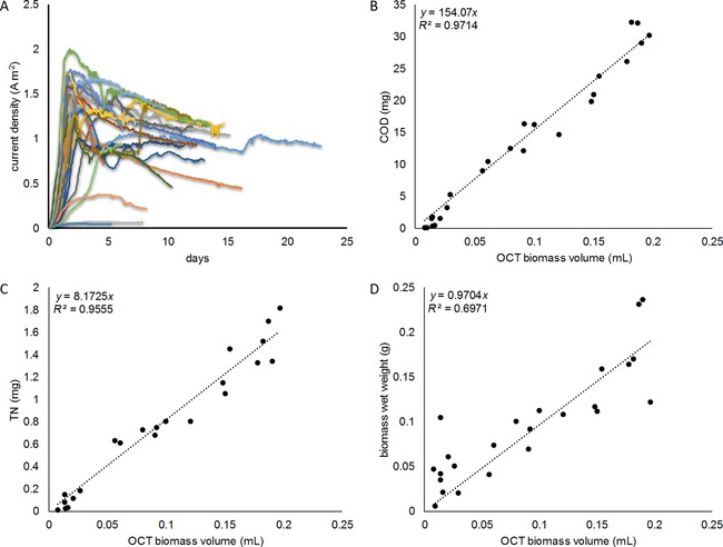
A) Current density development for the 24 individual runs. B) COD_Biomass, C) total N content (TN), and D) wet weight plotted versus the biomass volume as measured by OCT. COD and total N were normalized to the total FTO surface area, thus providing an absolute measure.

The obtained biofilm thicknesses ranged between 3 to 90 μm for all measured samples. Biomass volume as measured by OCT was calculated by multiplying the average biofilm thickness with the effective electrode area (22.3 cm²). Figure 1 B and C compare the obtained measured biofilm volumes to the total biofilm chemical oxygen demand (COD) and total nitrogen content, respectively. Both COD and total N show a strong linear relationship with biofilm volume as measured by OCT. With coefficients of determination well above 0.95, OCT showed itself to be a reliable estimator for both biofilm COD and N content in these experiments. From these data, the COD/N ratio was determined to be 18.7:1 by linear regression (R ²=0.97). Assuming a conversion ratio between COD and total organic carbon (TOC)54 of 3:1, this converts to a C/N ratio in the measured biomass of approximately 6:1, which is within the range of previously reported C/N ratios for microbial biomass.55 As a side note regarding the linearity between OCT and COD/total N, a tendency of OCT analysis to slightly overestimate biofilm volume in the lower volume region (0–0.02 mL) was observed. For the measurements in which only a very thin biofilm was present, a slightly increased but inevitable noise amplification occurred owing to (i) increased OCT autocorrelation artefacts associated with a clean FTO/electrolyte interface and (ii) increased noise amplification by the adaptive histogram equalization. These observations thus limit the precision of the presented method in this starting domain of early biofilm attachment and growth, but validate its use over a broader range of biofilm thicknesses.

To assess the accuracy of OCT for measuring absolute volumetric quantities of biomass, in Figure 1 D), the biomass volume as measured by OCT is plotted against the biomass wet pellet weight. Assuming a specific density of wet biomass similar to that of water (1 g L⁻¹), a 1:1 linear relationship would be expected between these two variables. The linear regression for these two variables indeed showed a slope of nearly 1, supporting the used method for measuring biomass volume in terms of its accuracy. The lower R ² value for this fit somewhat weakens this position, but it is to our best understanding the inevitable imprecisions and inaccuracies involved with weighing of small amounts of wet biomass—thus not the OCT methods applied—which created considerable additional variance, leading to this lower R ².

Determination of biomass growth yield by using a combination of OCT and chronoamperometry

Apart from biomass growth rates, the biomass growth yield, or yield ratio, is a parameter of importance in most BES studies. Biomass yield ratio defines to a great extent the energy efficiency and thus system performance, and is commonly expressed as gram COD biomass gained per gram of COD substrate consumed, with 1 mol of COD being equivalent to 4 mol of electrons. Accordingly, the yield ratio represents the number of electrons used for anabolism (creation of biomass) compared with the total amount of electrons derived from oxidizing the electron donor, including catabolism (substrate turnover for energy production required for growth).

Specifically for electrogenic biomass, the substrate consumed for catabolic processes is directly linked to current production. With biomass volume being linearly related to biomass COD (Figure 1 B), biomass growth yield can be assessed indirectly by plotting biofilm volume versus total charge produced during biofilm growth, and this is done in Figure 2.

Figure 2.

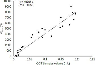
Scatter and regression slope of the measured biomass volume by OCT against the total amount of charge (Q _total) obtained from the biofilm.

We observed a good match between biofilm volume as measured by OCT and total charge: with more charge produced, biofilm volume increased. As can be inferred from this linearity, yields throughout the different runs were rather constant. This would be in line with growth conditions (and most notably anode potential) for each experiment being the same, and the biofilm being harvested being still in the growth stage (thus with none of the grown biomass being washed out or detached from the electrode, and no substantial changes or impact of maintenance on overall growth yields).

Elaborating on this assumption of linearity and constant growth yields, and to avoid error propagation in calculating yields from individual measurements, the overall yield of biomass on current was taken as the slope of the regression line: 1 mL biomass/40 705 C electrons. This value for V _biomass/Q (Q is the accumulated charge) was then inserted into Equations (6) and (7) (see Experimental Section), yielding 42.15 mg${}_{\mathrm{COD}{}_{\mathrm{biomass}}}$  g${}_{\mathrm{COD}{}_{\mathrm{acetate}}}$ ⁻¹ (coulombic efficiency (CE)=0.958). This obtained yield is a feasible value, being within range of earlier reported biomass yields27 and lower but comparable to the theoretical maximum biomass yield of 109 mg${}_{\mathrm{COD}{}_{\mathrm{biomass}}}$  g${}_{\mathrm{COD}{}_{\mathrm{acetate}}}$ ⁻¹ (CE=0.891) calculated at the used anode potential of −0.35 V by using the thermodynamic approach from Picioreanu et al.32 Thus, we show that by using a combination of OCT and chronoamperometric data—both noninvasive measurements—we can derive valid biomass growth yields from the tested systems.

Continuous measurement confirms application of OCT for noninvasive assessment of biofilm growth and activity

Two independent bioanodes were grown to confirm the applicability of OCT for tracking biofilm growth over time. Figure 3 shows the cumulative charge and OCT derived estimates for biofilm volume obtained from these two cells for which time‐lapse observations of biofilm growth were conducted. Figure 3 A shows the results for cell 1, which was operated for a total of 14 days, and Figure 3 B shows the results for the second cell, operated for a period of 17 days. From the measurements of biofilm volume and accompanying charge consumption, biomass yield estimates were obtained by linear regression. These are visualized for both cells in Figure 4, and the high R ² obtained strongly suggests a constant yield throughout the experimental period for both cells. The obtained yield estimates from these regressions for both cells were significantly similar to each other (38.7 and 38.8 mg${}_{\mathrm{COD}{}_{\mathrm{biomass}}}$  g${}_{\mathrm{COD}{}_{\mathrm{acetate}}}$ ⁻¹, p=0.976 under the null hypothesis of identical slopes), thus showing high reproducibility of the used methods.

Figure 3.

Development of charge (black) and biofilm volume (as measured by OCT, green, dashed, with markers) during two independent continuous experiments. In these experiments, cells were resumed to produce current after each OCT measurement. A) Results for a cell run for a total of 14 days. B) A cell in which the last OCT measurement was conducted at 17 days after the start.

Figure 4.

Relationship between accumulated charge and biomass volume as measured by OCT, providing a measure of yield, for both time‐lapse operated cells. In the above representation, the data for cell 2 for the periods in which cell conditions were unknown or fluctuating was removed. The straight lines (y1 in dashed orange for cell 1, y2 in solid black for cell 2) are obtained by linear regression, and the slopes resulting from these fits and their R ² values are included. The high correlation coefficients obtained strongly suggest constant yields throughout the experimental period. Yields were calculated from these obtained slopes to be 38.7 and 38.8 mg${}_{\mathrm{COD}{}_{\mathrm{biomass}}}$  g${}_{\mathrm{COD}{}_{\mathrm{acetate}}}$ ⁻¹ for cells 1 and 2, respectively, and an additional T‐test showed them to be significantly the same (p=0.976).

In general, current production resumed fast and completely after OCT measurements were performed and systems were electronically and hydraulically reconnected. However, upon reconnecting on day 9, inaccurate potential control for cell 2 led to the anode potential fluctuating between −0.35 and −0.45 V throughout the period of day 9 to 15. Over this period of fluctuating potential, an incremental yield estimate of 16 mg${}_{\mathrm{COD}{}_{\mathrm{biomass}}}$  g${}_{\mathrm{COD}{}_{\mathrm{acetate}}}$ ⁻¹ (CE=0.984) was obtained, roughly half as large as in the case of yields obtained when potential was controlled steadily at −0.35 V. Although unintended, this suggests fast adaptive behavior of the present biofilm to potential change. Owing to this artefact, this period was left out of the analysis as depicted in Figure 4.

Overall, the slightly lower yields obtained with the time‐lapse experiments compared with the sacrificial calibration experiments may be explained by the presence of periods during which cells were not connected to the potentiostat, leading to a slightly lower overall anode potential for the continuous runs.

Conclusions

We have demonstrated here that accurate and precise measurements of biomass volume can be obtained in situ and noninvasively from active bioanodes by using optical coherence tomography (OCT) in bioelectrochemical systems (BESs). This allows biomass yield and coulombic efficiency (CE) estimates to be obtained at high statistical precision and in real‐time. The method developed showed the OCT results to be linearly correlated to conventional biomass quantifications using chemical oxygen demand (COD) and total N content. As such, the presented method allows a more complete and meaningful characterization of BESs, especially when used in combination with additional in situ measurements such as pH value, off‐gas analysis, and/or electrolyte chemical analysis. When such characterizations are performed at different experimental conditions, this will provide valuable data for a deeper understanding of mechanisms at play in BESs, especially in the field of bioenergetics. It is anticipated to lead to identification of deviations from assumed thermodynamic model assumptions, or rate limiting factors/processes. Moreover, the used fluorine‐doped tin oxide (FTO) electrodes enable the concomitant application of different electrochemical and visualization techniques, for example, confocal Raman spectroscopy, confocal laser scanning microscopy, and more sophisticated electrochemical methods such as cyclic voltammetry and electrochemical impedance spectroscopy. These electrodes therefore provide ample opportunities for studying in‐depth the kinetic properties and mechanisms of electron transport in BESs, as well as allowing for high‐resolution visualization and functionalized imaging of living biofilms.

Experimental Section

Reactor setup

Electrochemical cells consisted of two Plexiglas plates with flow channels (33 cm³) separated by a bipolar membrane (Ralex PE‐BPM, MEGA a.s., Czech Republic). FTO‐coated glass slides (22.3 cm² exposed anode area) were used as anodes for the biofilm to attach to and grow on. Anode current collectors were made of graphite paper sheets, from which the flow channel area was extruded. By extruding the flow channel from the current collector, the graphite paper was touching the FTO layer only in places where no electrolyte was present. A flat sheet of stainless steel (316 alloy) lined with a sheet of carbon paper was used as a cathode. Figure 5 shows a photographic overview of the constructed cells. Ag/AgCl reference electrodes (Prosense, Oosterhout, The Netherlands; +0.203 V vs. standard hydrogen electrode) were inserted into the anode chamber via a Haber–Luggin capillary filled with a saturated solution of KCl and all potentials are expressed with respect to this electrode.

Figure 5.

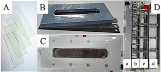
Photographic overview of the used cell components and their assembly showing A) FTO electrodes, B) anode end plate, graphite current collector, and neoprene gasket (from top to bottom), C) top view of the anode compartment with exposed face of FTO electrode in the middle, D) completely assembled cell with clearly visible: a) anode end plate, b) anode flow compartment, c) cathode flow compartment, d) cathode end plate.

Reactor inoculation and operation

Reactors were inoculated with biomass from active acetate oxidizing bioanodes. The influent consisted of (g L⁻¹): 0.74 KCl, 0.58 NaCl, 3.4 KH₂PO₄, 4.35 K₂HPO₄, 0.28 NH₄Cl, 0.1 MgSO₄ ⋅7 H₂O, 0.1 CaCl₂ ⋅2 H₂O, 0.82 sodium acetate, 2.1 sodium 2‐bromoethanesulfonate, 1 mL trace metal mixture, and 1 mL vitamins mixture according to DSMZ culture medium 141 (chemicals obtained from VWR and of technical grade or higher).53 The influent stock solution was continuously sparged with N₂ before being fed to the reactor to maintain anaerobic conditions. The influent was fed to the reactor at a rate of 0.16 mL min⁻¹ (hydraulic retention time HRT=20 h, total recirculated anolyte volume=200 mL). The catholyte initially consisted of 10 mm phosphate buffer at pH 7, which was not replaced between experimental runs. The catholyte was continuously sparged with N₂ to strip it of any formed hydrogen gas.

Experimental design

The use of OCT for biofilm quantification was validated by conducting a total of 24 runs, where each run started with a clean FTO anode. The anode potential during each run was controlled at −350 mV with a potentiostat (N‐stat d‐module, Ivium Technology, The Netherlands). To bring variation to the amount of biofilm at sampling, a temporally equally spaced sampling schedule was chosen in which runs produced current between 1 up to 24 days before sampling. Just before the end of a run, reactors were assessed by OCT. They were then dismantled and the biofilm was harvested for further chemical analyses.

The use of OCT for noninvasive time‐lapse observations of biofilm development was tested and illustrated. To this end, two cells were constructed and operated as above, but instead of being harvested after OCT, these cells were reconnected and their operation was continued. Moreover, regarding the influent for these systems, acetate was separated from other nutrients to improve substrate loading stability. To analyze these systems by OCT, they were disconnected both hydraulically and electronically for approximately two hours each time the system was sampled. Sampling periodicity was defined pragmatically, aiming for a comparable amount of charge to have passed between measurement points. In total, this practice was carried for 14 days for one, and 17 days for the other cell.

OCT acquisition and image processing

In situ imaging of the FTO anode was performed by using a spectral domain optical coherence tomograph (Thorlabs Ganymede SD‐OCT System). To get a representative dataset regarding the distribution of biofilm on the electrode, the OCT measurement was performed at 54 predefined, evenly distributed spots (see Figure 6), by using an automated translation stage (Thorlabs LTS300&150/M). The axial (i.e., perpendicular to the anode) spatial resolution for the OCT instrument is below 5.8 μm, and the lateral (i.e., parallel to the electrode) resolution is 8 μm. The OCT was fitted with a 5× telecentric scan lens (Thorlabs LSM03BB), configured to make a “B scan” (horizontal line scan) consisting of 1000 equally spaced “A scans” (depth scans) over a 1 mm transect by using the instrument's software. See Figure 6 for a schematic overview of the acquisition method used. Based on these scan settings and on an assumed bulk refractive index of 1.33 (identical to that of water), two‐dimensional cross‐sectional images were acquired max. 2.1 mm deep at a pixel dimension of 1×2.05 μm (lateral–axial).

Figure 6.

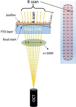
Schematic overview of the acquisition method used for the OCT. A single B scan was composed of 1000 A scans. On the right, a schematic FTO electrode with biofilm is depicted. The 54 individual B scans taken from predefined spots during OCT analysis are indicated by black lines.

The used acquisition method, including data export, had a total processing time of roughly 40 seconds per site. More details on the specific acquisition parameters of the OCT can be found in the Supporting Information.

Post‐processing consisted of converting scan data into 32‐bit floating point CSV files by using the instrument's software. Data was imported, normalized, and further processed by using a custom MATLAB script (MATLAB 2017b using the built‐in image processing toolbox). Images were processed by a multi‐step sequence: (1) image contrast was improved and equalized by applying contrast‐limited adaptive histogram equalization (CLAHE) by using the “adapthisteq” function (Figure 7 A); (2) the position of the lower part of the FTO layer (interfacing with the biofilm) was determined. Assuming an (almost) perpendicular positioning of the FTO layer with respect to the scan direction, a row vector was calculated, containing the mean for each row. Differences between adjacent rows from this row vector were calculated, and the row containing the minimal (most negative) resulting difference was determined. After the determination of this row number, a mask of zeros was applied to the image for all the pixels above that row number, removing the FTO electrode image and everything above, that is, electrolyte (Figure 7 B); (3) To isolate the biomass structure, edge detection (Sobel method) was used. This returned edges at those points where the gradient on the picture was above a set threshold value; (4) Since the edge detection led to some noise amplification, two consecutive operations were performed to remove this: rows for which the row‐sum was higher than a threshold value were set to zero. Then, edges with more than 100 connected pixels were removed. What remained was a binary contour image of (presumably) only the biofilm, containing holes and breaches (Figure 7 C); (5) Breaches were closed by using the dilate function (imdilate, Figure 7 D), after which holes were filled with the built‐in function “imfill”. Some noise below the biofilm was still visible at this point (Figure 7 E); (6) As the last polishing steps, all objects smaller than 30 pixels were removed and the pixel value of the last two rows were set to zero. The latter was done to correct for artificial noise created by the edge detection step (Figure 7); (7) In the obtained binary picture, true pixels (value 1) represented the biomass. The pixel counts for each of the 54 cross‐sections analyzed per electrode were then averaged and the average biofilm thickness was obtained by dividing the average pixel count by the lateral pixel scaling factor. Biofilm volume was calculated by multiplying the average biofilm thickness with the electrode surface area. The complete MATLAB script is disclosed in the Supporting Information.

Figure 7.

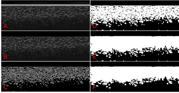
Step‐by‐step visualization of the image processing involved with OCT analysis. A) Image after adaptive histogram equalization, clearly depicting the bright FTO layer on top of the image. B) FTO layer and all above removed. C) Binary image after edge‐detection. D) After “gluing” of detected edges. E) After filling holes. F) After removing loose and small particles.

Chemical analyses

After dismantling the cell, the biofilm was first gently rinsed with a 100 mm phosphate buffer solution to remove residual soluble organics, chloride, and ammonium while preventing acute osmotic stress. The biofilm was then mechanically detached from the glass electrode by using a conventional cell scraper. The wet biomass pellet weight was measured and then suspended with the use of vortex and sonication in a defined volume (10 mL of 100 mm phosphate buffer solution). The resulting homogenized samples were analyzed for COD and total nitrogen content by using photometric test kits (Hach‐Lange LCK 114 and 138, respectively). Assuming a volumetric density of 1 g mL⁻¹ for wet biomass, the absolute amounts of COD and total N for each electrode were then calculated.

Calculations and conversions used to obtain biomass growth yield

Assuming biomass formation as the only competing process to current generation from acetate oxidation, we can express the electron balance in our systems as Equation (1):

$${\displaystyle e{}_{\mathrm{electrode}}+e{}_{\mathrm{biomass}}=-e{}_{\mathrm{substrate}}}$$ (1)

In this simple expression, e _electrode represents the number of electrons channeled to the electrode, thus representing catabolic activity of the present biomass. e _biomass equals the number of electrons that ends up in the formation of biomass, thus representing anabolic activity.

The electrons expressed as −e _substrate are derived from substrate oxidation (acting as electron donor, negative by convention).

The yield coefficient (Y), by convention, expresses the ratio of electrons used for biomass growth (i.e., anabolism) to electrons derived from substrate oxidation [Eq. (2)]:

$${\displaystyle Y=\frac{e_{\mathrm{b}\mathrm{i}\mathrm{o}\mathrm{m}\mathrm{a}\mathrm{s}\mathrm{s}}}{{-e}_{\mathrm{s}\mathrm{u}\mathrm{b}\mathrm{s}\mathrm{t}\mathrm{r}\mathrm{a}\mathrm{t}\mathrm{e}}}}$$ (2)

To determine the biomass growth yield, we used the biomass volume from the presented OCT measurements in combination with the total produced charge (as measured by chronoamperometry). First, the biomass volume as measured by OCT (V _biomass [mL]) was converted into COD_biomass [g_COD] by using a linear correlation established in this study [Eq. (3); (Figure 1 B)]

$${\displaystyle \mathrm{COD}{}_{\mathrm{biomass}}=\alpha V{}_{\mathrm{biomass}}}$$ (3)

with α being the regression coefficient.

The obtained COD_biomass was then converted into e _biomass [mol] using Equation (4):

$${\displaystyle e_{\mathrm{b}\mathrm{i}\mathrm{o}\mathrm{m}\mathrm{a}\mathrm{s}\mathrm{s}}=\frac{n{\mathrm{C}\mathrm{O}\mathrm{D}}_{\mathrm{b}\mathrm{i}\mathrm{o}\mathrm{m}\mathrm{a}\mathrm{s}\mathrm{s}}}{M_{{\mathrm{O}}_2}}}$$ (4)

in which M ${}_{\mathrm{O}{}_2}$ is the molecular weight of dioxygen (32 g) and n is the electron stoichiometry involved with complete reduction of dioxygen (n=4).

The accumulated charge (Q) on the electrode (electron acceptor) is expressed in e by division with the Faraday constant (F) [Eq. (5)]

$${\displaystyle e_{\mathrm{e}\mathrm{l}\mathrm{e}\mathrm{c}\mathrm{t}\mathrm{r}\mathrm{o}\mathrm{d}\mathrm{e}}=\frac{Q}{F}}$$ (5)

Thus, by combining Equations (1)–(5), Equation (6) is obtained:

$${\displaystyle Y=\frac{e_{\mathrm{b}\mathrm{i}\mathrm{o}\mathrm{m}\mathrm{a}\mathrm{s}\mathrm{s}}}{e_{\mathrm{e}\mathrm{l}\mathrm{e}\mathrm{c}\mathrm{t}\mathrm{r}\mathrm{o}\mathrm{d}\mathrm{e}}+e_{\mathrm{b}\mathrm{i}\mathrm{o}\mathrm{m}\mathrm{a}\mathrm{s}\mathrm{s}}}=\frac{1}{1+\frac{e_{\mathrm{e}\mathrm{l}\mathrm{e}\mathrm{c}\mathrm{t}\mathrm{r}\mathrm{o}\mathrm{d}\mathrm{e}}}{e_{\mathrm{b}\mathrm{i}\mathrm{o}\mathrm{m}\mathrm{a}\mathrm{s}\mathrm{s}}}}=\frac{1}{\left(1+\frac{M_{{\mathrm{O}}_2}Q}{\alpha {nFV}_{\mathrm{b}\mathrm{i}\mathrm{o}\mathrm{m}\mathrm{a}\mathrm{s}\mathrm{s}}}\right)}}$$ (6)

Moreover, as by convention coulombic efficiency (CE) is defined as the ratio of the number of electrons channeled to the acceptor (e _electrode) with the number of electrons derived from substrate oxidation (e _substrate), by using Equation (5) the following definition for CE is obtained [Eq. (7)]:

$${\displaystyle \mathrm{C}\mathrm{E}=\frac{e_{\mathrm{e}\mathrm{l}\mathrm{e}\mathrm{c}\mathrm{t}\mathrm{r}\mathrm{o}\mathrm{d}\mathrm{e}}}{-e_{\mathrm{s}\mathrm{u}\mathrm{b}\mathrm{s}\mathrm{t}\mathrm{r}\mathrm{a}\mathrm{t}\mathrm{e}}}=1-Y}$$ (7)

It should be noted here, however, in case CE is defined on basis of biomass production measurements, this can only reflect a theoretical maximally attainable CE. Actual CEs may be lower if unreported side processes not leading to detected biomass growth are also present.

Conflict of interest

The authors declare no conflict of interest.

Supporting information

As a service to our authors and readers, this journal provides supporting information supplied by the authors. Such materials are peer reviewed and may be re‐organized for online delivery, but are not copy‐edited or typeset. Technical support issues arising from supporting information (other than missing files) should be addressed to the authors.

Supplementary

S. D. Molenaar, T. Sleutels, J. Pereira, M. Iorio, C. Borsje, J. A. Zamudio, F. Fabregat-Santiago, C. J. N. Buisman, A. ter Heijne, ChemSusChem 2018, 11, 2171.

References

- 1. Lovley D. R., Energy Environ. Sci. 2011, 4, 4896–4906. [Google Scholar]
- 2. Reguera G., McCarthy K. D., Mehta T., Nicoll J. S., Tuominen M. T., Lovley D. R., Nature 2005, 435, 1098–1101. [DOI] [PubMed] [Google Scholar]
- 3. Lovley D. R., Annu. Rev. Microbiol. 2012, 66, 391–409. [DOI] [PubMed] [Google Scholar]
- 4. Molenaar S. D., Mol A. R., Sleutels T. H. J. A., ter Heijne A., Buisman C. J. N., Environ. Sci. Technol. Lett. 2016, 3, 144–149. [Google Scholar]
- 5. Deeke A., Sleutels T. H. J. A., Hamelers H. V. M., Buisman C. J. N., Environ. Sci. Technol. 2012, 46, 3554–3560. [DOI] [PubMed] [Google Scholar]
- 6. Logan B. E., Hamelers B., Rozendal R., Schröder U., Keller J., Freguia S., Aelterman P., Verstraete W., Rabaey K., Environ. Sci. Technol. 2006, 40, 5181–5192. [DOI] [PubMed] [Google Scholar]
- 7. Logan B. E., Call D., Cheng S., Hamelers H. V. M., Sleutels T. H. J. A., Jeremiasse A. W., Rozendal R. A., Environ. Sci. Technol. 2008, 42, 8630–8640. [DOI] [PubMed] [Google Scholar]
- 8. Ledezma P., Kuntke P., Buisman C. J. N., Keller J., Freguia S., Trends Biotechnol. 2015, 33, 214–220. [DOI] [PubMed] [Google Scholar]
- 9. Rabaey K., Rozendal R. A., Nat. Rev. Microbiol. 2010, 8, 706–716. [DOI] [PubMed] [Google Scholar]
- 10. Logan B. E., Rabaey K., Science 2012, 337, 686–690. [DOI] [PubMed] [Google Scholar]
- 11. Donovan C., Dewan A., Heo D., Beyenal H., Environ. Sci. Technol. 2008, 42, 8591–8596. [DOI] [PubMed] [Google Scholar]
- 12. Strik D. P. B. T. B., Timmers R. A., Helder M., Steinbusch K. J. J., Hamelers H. V. M., Buisman C. J. N., Trends Biotechnol. 2011, 29, 41–49. [DOI] [PubMed] [Google Scholar]
- 13. Stein N. E., Keesman K. J., Hamelers H. V. M., van Straten G., Biosens. Bioelectron. 2011, 26, 3115–3120. [DOI] [PubMed] [Google Scholar]
- 14. Su L., Jia W., Hou C., Lei Y., Biosens. Bioelectron. 2011, 26, 1788–1799. [DOI] [PubMed] [Google Scholar]
- 15. Malvankar N. S., Mester T., Tuominen M. T., Lovley D. R., ChemPhysChem 2012, 13, 463–468. [DOI] [PubMed] [Google Scholar]
- 16. Liu Y., Bond D. R., ChemSusChem 2012, 5, 1047–1053. [DOI] [PMC free article] [PubMed] [Google Scholar]
- 17. Freguia S., Rabaey K., Yuan Z., Keller J., Environ. Sci. Technol. 2007, 41, 2915–2921. [DOI] [PubMed] [Google Scholar]
- 18. Lovley D. R., Curr. Opin. Biotechnol. 2008, 19, 564–571. [DOI] [PubMed] [Google Scholar]
- 19. Marsili E., Baron D. B., Shikhare I. D., Coursolle D., Gralnick J. A., Bond D. R., Proc. Natl. Acad. Sci. USA 2008, 105, 3968–3973. [DOI] [PMC free article] [PubMed] [Google Scholar]
- 20. Torres C. I., Marcus A. K., Rittmann B. E., Biotechnol. Bioeng. 2008, 100, 872–881. [DOI] [PubMed] [Google Scholar]
- 21. Kracke F., Vassilev I., Krömer J. O., Front. Microbiol. 2015, 6, 10.3389/fmicb.2015.00575. [DOI] [PMC free article] [PubMed] [Google Scholar]
- 22. ter Heijne A., Schaetzle O., Gimenez S., Navarro L., Hamelers B., Fabregat-Santiago F., Bioelectrochemistry 2015, 106, 64–72. [DOI] [PubMed] [Google Scholar]
- 23. Zhi W., Ge Z., He Z., Zhang H., Bioresour. Technol. 2014, 171, 461–468. [DOI] [PubMed] [Google Scholar]
- 24. Logan B. E., ChemSusChem 2012, 5, 988–994. [DOI] [PubMed] [Google Scholar]
- 25. Rozendal R. A., Hamelers H. V. M., Rabaey K., Keller J., Buisman C. J. N., Trends Biotechnol. 2008, 26, 450–459. [DOI] [PubMed] [Google Scholar]
- 26. Sleutels T. H. J. A., Ter Heijne A., Buisman C. J. N., Hamelers H. V. M., ChemSusChem 2012, 5, 1012–1019. [DOI] [PubMed] [Google Scholar]
- 27. Aelterman P., Freguia S., Keller J., Verstraete W., Rabaey K., Appl. Microbiol. Biotechnol. 2008, 78, 409–418. [DOI] [PubMed] [Google Scholar]
- 28. Wei J., Liang P., Cao X., Huang X., Environ. Sci. Technol. 2010, 44, 3187–3191. [DOI] [PubMed] [Google Scholar]
- 29. Yates M. D., Kiely P. D., Call D. F., Rismani-Yazdi H., Bibby K., Peccia J., Regan J. M., Logan B. E., ISME J. 2012, 6, 2002–2013. [DOI] [PMC free article] [PubMed] [Google Scholar]
- 30. Read S. T., Dutta P., Bond P. L., Keller J., Rabaey K., BMC Microbiol. 2010, 10, 98. [DOI] [PMC free article] [PubMed] [Google Scholar]
- 31. Sleutels T. H. J. A., Darus L., Hamelers H. V. M., Buisman C. J. N., Bioresour. Technol. 2011, 102, 11172–11176. [DOI] [PubMed] [Google Scholar]
- 32. Picioreanu C., Head I. M., Katuri K. P., van Loosdrecht M. C. M., Scott K., Water Res. 2007, 41, 2921–2940. [DOI] [PubMed] [Google Scholar]
- 33. Hamelers H. V. M., Ter Heijne A., Stein N., Rozendal R. A., Buisman C. J. N., Bioresour. Technol. 2011, 102, 381–387. [DOI] [PubMed] [Google Scholar]
- 34. Rodríguez J., Lema J. M., Kleerebezem R., Trends Biotechnol. 2008, 26, 366–374. [DOI] [PubMed] [Google Scholar]
- 35. Franks A. E., Malvankar N., Nevin K. P., Biofuels 2010, 1, 589–604. [Google Scholar]
- 36. Khan M. R., Baranitharan E., Prasad D. M. R., Cheng C. K., MATEC Web of Conferences, 2016, 16, 04002. [Google Scholar]
- 37. Jourdin L., Grieger T., Monetti J., Flexer V., Freguia S., Lu Y., Chen J., Romano M., Wallace G. G., Keller J., Environ. Sci. Technol. 2015, 49, 13566–13574. [DOI] [PubMed] [Google Scholar]
- 38. Chen L., Tremblay P.-L., Mohanty S., Xu K., Zhang T., J. Mater. Chem. A 2016, 4, 8395–8401. [Google Scholar]
- 39. Katuri K. P., Enright A. M., O'Flaherty V., Leech D., Bioelectrochemistry 2012, 87, 164–171. [DOI] [PubMed] [Google Scholar]
- 40. Molenaar S. D., Saha P., Mol A. R., Sleutels T. H. J. A., ter Heijne A., Buisman C. J. N., Int. J. Mol. Sci. 2017, 18, 204. [DOI] [PMC free article] [PubMed] [Google Scholar]
- 41. Franks A. E., Nevin K. P., Jia H., Izallalen M., Woodard T. L., Lovley D. R., Energy Environ. Sci. 2009, 2, 113–119. [Google Scholar]
- 42. Kim G. T., Webster G., Wimpenny J. W. T., Kim B. H., Kim H. J., Weightman A. J., J. Appl. Microbiol. 2006, 101, 698–710. [DOI] [PubMed] [Google Scholar]
- 43. Kim B. H., Park H. S., Kim H. J., Kim G. T., Chang I. S., Lee J., Phung N. T., Appl. Microbiol. Biotechnol. 2004, 63, 672–681. [DOI] [PubMed] [Google Scholar]
- 44. Lawrence J. R., Neu T. R., Methods Enzymol. 1999, 310, 131–144. [DOI] [PubMed] [Google Scholar]
- 45. Neu T. R., Manz B., Volke F., Dynes J. J., Hitchcock A. P., Lawrence J. R., FEMS Microbiol. Ecol. 2010, 72, 1–21. [DOI] [PubMed] [Google Scholar]
- 46. Kamjunke N., Spohn U., Füting M., Wagner G., Scharf E. M., Sandrock S., Zippel B., Int. Biodeterior. Biodegrad. 2012, 69, 17–22. [Google Scholar]
- 47. Ding Y., Zhou Y., Yao J., Szymanski C., Fredrickson J., Shi L., Cao B., Zhu Z., Yu X.-Y., Anal. Chem. 2016, 88, 11244–11252. [DOI] [PubMed] [Google Scholar]
- 48. Virdis B., Harnisch F., Batstone D. J., Rabaey K., Donose B. C., Energy Environ. Sci. 2012, 5, 7017–7024. [Google Scholar]
- 49. Huang D., Swanson E. A., Lin C. P., Schuman J. S., Stinson W. G., Chang W., Hee M. R., Flotte T., Gregory K., Puliafito C. A., Fujimoto J. G., Science 1991, 254, 1178–1181. [DOI] [PMC free article] [PubMed] [Google Scholar]
- 50. Dreszer C., Wexler A. D., Drusová S., Overdijk T., Zwijnenburg A., Flemming H. C., Kruithof J. C., Vrouwenvelder J. S., Water Res. 2014, 67, 243–254. [DOI] [PubMed] [Google Scholar]
- 51. ter Heijne A., Hamelers H. V. M., Saakes M., Buisman C. J. N., Electrochim. Acta 2008, 53, 5697–5703. [Google Scholar]
- 52. Dekker A., ter Heijne A., Saakes M., Hamelers H. V. M., Buisman C. J. N., Environ. Sci. Technol. 2009, 43, 9038–9042. [DOI] [PubMed] [Google Scholar]
- 53.Deutsche Sammlung von Mikroorganismen und Zellkulturen, 141. Methanogenium Medium (H2/CO2), https://www.dsmz.de/microorganisms/medium/pdf/DSMZ_Medium141.pdf, (accessed 20 February 2018).
- 54. Dubber D., Gray N. F., J. Environ. Sci. Health Part A 2010, 45, 1595–1600. [DOI] [PubMed] [Google Scholar]
- 55. Vassilev S. V., Baxter D., Andersen L. K., Vassileva C. G., Fuel 2010, 89, 913–933. [Google Scholar]
Associated Data
This section collects any data citations, data availability statements, or supplementary materials included in this article.
Supplementary Materials