Correlated Regression Feature Learning for Automated Right Ventricle Segmentation

Abstract

Accurate segmentation of right ventricle (RV) from cardiac magnetic resonance (MR) images can help a doctor to robustly quantify the clinical indices including ejection fraction. In this paper, we develop one regression convolutional neural network (RegressionCNN) which combines a holistic regression model and a convolutional neural network (CNN) together to determine boundary points’ coordinates of RV directly and simultaneously. In our approach, we take the fully connected layers of CNN as the holistic regression model to perform RV segmentation, and the feature maps extracted by convolutional layers of CNN are converted into 1-D vector to connect holistic regression model. Such connection allows us to make full use of the optimization algorithm to constantly optimize the convolutional layers to directly learn the holistic regression model in the training process rather than separate feature extraction and regression model learning. Therefore, RegressionCNN can achieve optimally convolutional feature learning for accurately catching the regression features that are more correlated to RV regression segmentation task in training process, and this can reduce the latent mismatch influence between the feature extraction and the following regression model learning. We evaluate the performance of RegressionCNN on cardiac MR images acquired of 145 human subjects from two clinical centers. The results have shown that RegressionCNN’s results are highly correlated (average boundary correlation coefficient equals 0.9827) and consistent with the manual delineation (average dice metric equals 0.8351). Hence, RegressionCNN could be an effective way to segment RV from cardiac MR images accurately and automatically.

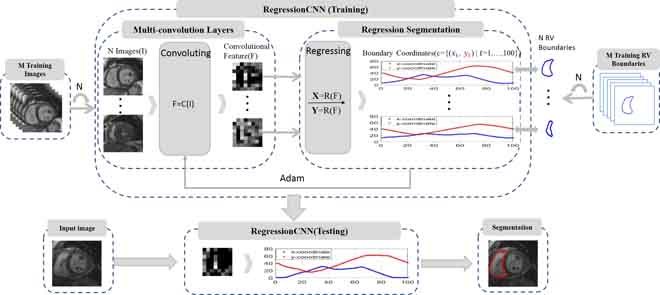
The overview of the proposed RegressionCNN framework. RegressionCNN takes RV segmentation as a regression task. The RegressionCNN uses multi-convolution layers to extract features from cardiac images. Then the fully-connected layers as the holistic regression model is used to estimate all boundary points' coordinates of RV directly and simultaneously in a unified framework.

I. Introduction

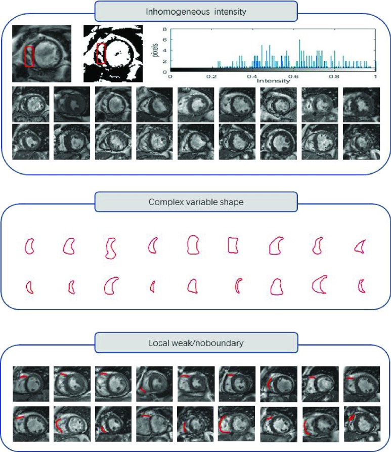
A number of studies have showed the RV is of high importance for maintaining the hemodynamic stability and cardiac performance [1]–[3]. Accurate assessment of RV structure and function can help to monitor related cardiac disorders including pulmonary hypertension and coronary cardiac disease [4]. Segmentation of RV is the first step to acquire the evaluation of RV structure and function [5]. Manual delineation of border by physician is still standard clinical procedure now. However, manual segmentation is not only time-consuming process, but also prone to intra- and inter-observer variability [6]. Therefore, it is of great importance to develop computer-aided algorithm to automatically acquire RV border to facilitate the evaluation process. Many previous computer-aided segmentation methods have been proposed to segment RV. However, the problems like the complex variable crescent shape, local weak/no boundary and inhomogeneous intensity of RV bring great challenges to these computer-aided methods [7]–[9] (as shown in Fig.1). For instance, Model-based methods and atlas-guided methods are sensitive to complex variable shapes of RV. Model-based methods rely on the training data to construct a model [10]. Due to the complex variable shapes of RV and limited data, the training data is always not representative enough for all possible RV shapes and variations to achieve high accuracy. The atlas-guide methods leverage the atlas as a reference frame for segmenting new images [11], [12]. Because of anatomical variability, accurate segmentation of complex variable RV is difficult. Intensity-based methods are sensitive to inhomogeneous intensity profiles and inhomogeneous intensity distribution inside RV [13]–[15]. The inhomogeneous intensity can bring a noise disturbance when seeking the optimal region partition. Therefore, intensity-based methods can be easily confused or seek a false region partition of RV. Deformable models rely on edges to evolve boundary [16]–[19]. They are sensitive to local weak/no boundary as it breaks the required assumption which considers boundaries is clearly visible. Deformable models can leak the true boundary of RV, and fail to evolve the true boundary at the location of weak/no boundaries. Furthermore, the complex variable crescent shape, local weak/no boundary and inhomogeneous intensity of RV always appear at the same time, which pose a greater challenge to these methods. Therefore, it is very necessary to enhance the robustness and accuracy of methods by simultaneously dealing with complex variable crescent shape, local weak/no boundary and inhomogeneous intensity of RV.

FIGURE 1.

The complexities of RV: inhomogeneous intensity, complex variable shape, local weak/no boundary.

The recently proposed regression-based segmentation approach is an appropriate strategy to simultaneously tackle the complex variable shape, local weak/no boundary and inhomogeneous intensity of object. And it presents great segmentation performance in medical image segmentation [20]–[22]. Regression segmentation leverages the advantages of multi-output regression to simultaneously estimate the boundary points’ coordinates of object [23], [24]. Because the boundary points have spatial coherence and statistical correlation. The holistic regression segmentation can obtain more accurate estimation by learning a nonlinear multi-output regressor. Besides, holistic regression output fashion makes full use of input image and global shape prior to simultaneously guide regression [21]. Therefore, holistic regression segmentation obtains the accurate desired boundary by using the input image and the learned global shape prior to simultaneously regress boundary points’ coordinates. It does not need to rely on the information about edge or intensity and using single-output regressor to regress boundary points’ coordinates one by one. This is able to deal with local weak/no boundaries and inhomogeneous intensity of object naturally. In addition, the complex variable shape of object can be tackled by regressing each boundary point [22]. As a result, the holistic regression segmentation achieves the improved robustness and accuracy by simultaneously regressing all boundary points using the guidance of input image and global shape prior.

However, current existing holistic regression segmentation methods are based on two-phase segmentation They are separate feature extraction and regression model learning [20]–[22]. The two-phase segmentation methods need extra methods to extract features from all images before learning regression model such as multi-dimensional support vector regression (MSVR) [23] and multi-layer perception (MLP) [25]. Apparently, these two-phase segmentation methods lose the correlation between feature extraction and regression model learning. This can give rise to the latent mismatch influence between the feature extraction and regression model learning. Consequently, it is worthwhile to investigate a unified regression approach for more accurate RV segmentation. The approach not only should directly utilize input images and learned global shape prior to guide segmentation, but also is able to integrate feature extraction and regression model learning into one step.

Because convolutional layers of CNN can naturally follow by fully-connected layers, deconvolution layers and other task models. CNN is able to naturally integrate convolutional feature extraction and these task models into one unified framework [26]–[28]. It can establish a strong relationship between convolutional feature extraction and task models learning. Besides, CNN leverages convolutional layers to directly map input image to high-level abstraction space. In the high-level abstraction space, CNN learns similar features at different local area of image by convolutional operations. This can capture complex correlations at different local area [29], which gives rise to extracted shape information. Therefore, CNN can extract global shape prior to directly train a model to perform relevant task in a unified framework.

Hence, in this paper, we proposed RegressionCNN that combines the CNN and holistic regression model to estimate all boundary points’ coordinates of RV directly and simultaneously. It takes RV segmentation as a regression task. RegressionCNN is very effective to leverage input image and global shape prior to directly train regression model in a unified segmentation framework (as shown in Fig.2). It can result in that extracted features are correlated to regression segmentation model. In summary, the advantages of our proposed RegressionCNN are as follows: (1) our proposed RegressionCNN takes the RV segmentation as a holistic boundary regression task to utilize the advancement of CNN for seeking the optimal segmentation. Therefore, RegressionCNN leverages the entire image as input to regress each point. This can tackle complex variable crescent shape of RV, and enable each boundary point to detect its context to achieve accurate RV segmentation. Besides, RegressionCNN relies on input images and global shape prior to estimate all RV boundary points rather than depending on the information about edge or intensity. This can naturally tackle local weak/no boundary and inhomogeneous intensity of RV. (2) RegressionCNN integrates the feature extraction and regression segmentation into one step by the seamless connection of convolutional layers and holistic regression model. Such seamless connection gives rise to an optimally convolutional feature extraction for accurately catching the features that are more relevant to RV segmentation task. Besides, based on such connection, RegressionCNN makes full use of convolutional features to directly guide following regression model learning of fully-connected layers in a unified framework. This can reduce the latent mismatch influence between the feature extraction and regression model learning and simplify the RV segmentation work. (3) RegressionCNN simultaneously regresses a few points, which approximatively represent RV boundary. These points provide a flexible RV boundary representation to catch the diversity of RV boundaries.

FIGURE 2.

The overview of our proposed RegressionCNN. RegressionCNN integrates convolutional feature extraction and holistic regression segmentation model into a unified framework. The cardiac MR images input to the framework directly, and get desired RV boundary.

II. Methods

A. RV Boundary Representation

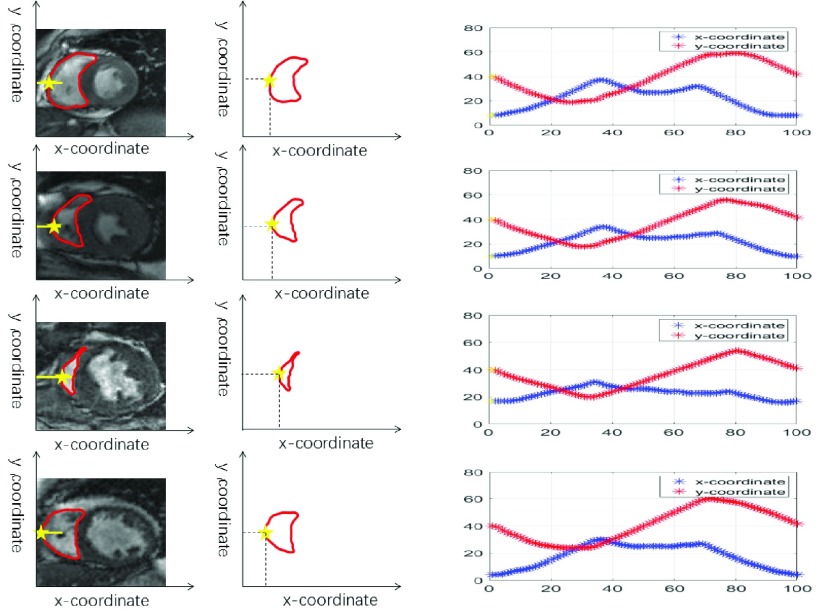
In our proposed RegressionCNN, we leverage 100 points to represent RV boundary, and is the k-th RV boundary point’s coordinates (as shown in Fig.3). To get the coordinates of boundary points in the same standard, we have the fixed size images in both training and testing processes. For each RV boundary, the points are obtained in a consistent way as following: first, we use matlab2015b to get all boundary points’ coordinates of RV based on manual delineation. Next, according to these points’ coordinates, the algorithm of cubic non-uniform B-spline interpolation is utilized to fit a curve of RV contour. Finally, we take 100 points evenly as the RV boundary on the fitted curve. The first point is selected at the location where the RV left boundary is crossed by the horizontal line whose coordinate is 40. And the rest are evenly sampled along the RV boundary in the counterclockwise direction. Therefore, our RV boundary representation can smoothly approximate RV complex shapes.

FIGURE 3.

RV boundary representation. We use 100 points to represent RV boundary approximately. The first point is that the RV left boundary is crossed by the horizontal line whose coordinate is 40 (yellow star). Each row illustrates the representation of normal, inhomogeneous intensity, complex variable shape and local weak/no boundaries of RV.

We use this kind of way to process the data because the RV size is different. If a large RV is represented by less boundary points, some local boundaries of RV can be lost. If a small RV is represented by many boundary points, it will increase the complexity in network. So, we have tested different numbers of points to represent RV. And finally, we found the number of 100 points not only represent the RV of different size better, but also do not increase much complexity. In many case that the number of boundary pixels of RV are less than 100 pixels, but we can obtain the 100 points from the fitted curve.

B. RegressionCNN: Regression Convolutional Neuron Network

RegressionCNN combines CNN and holistic regression model into a unified segmentation framework (as shown in Fig.2). In the unified framework, RegressionCNN uses the multi-convolutional layers to extract convolutional features to directly guide regression segmentation of fully-connected layers.

1). Multi-Convolutional Layers

In the first step, we attempt to extract the convolutional features from cardiac MR images. There are 3 convolutional layers that each follows by a max-pooling layer to extract convolutional features. We leverage the last pooling convolutional feature maps to guide segmentation. The convolutional kernels of the three convolutional layers are 16, 24, 32, respectively. The size of the convolutional kernel is . The max-pooling window of all max-pooling layers is . Due to Rectified Linear Units (RELU) is able to avoid the vanishing gradient problem and learning non-linear features [30], we use it as the activation function of convolutional layers. The first convolutional layer directly processes input images to extract low-level feature maps. Following layers process the feature maps of previous layers’ output to detect higher-level feature maps. By the learning of multiple layers, RegressionCNN can extract robust RV features from MR images regardless of noise’s influence. The n-th feature map (size is ) obtained from m-th convolutional layer is calculated by

Where is the feature map of upper layer, is the number of convolutional kernels, is the n-th convolutional kernel (size is ), is the activation function, is the bias. The equation (1) shows each neuron in convolutional layer connects to local area called receptive field in the feature map of upper layer through a group of same weights (convolutional kernel). Therefore, neurons in convolutional layer learn local similar features and capture complex correlations at different local area. This can not only learn global shape priors from cardiac MR images, but also can cut down numerous network parameters, resulting in reduced network complexity.

The convolutional feature maps are directly processed by max-pooling layers to obtain pooled feature maps. In our proposed RegressionCNN, a max-pooling window is used to select the maximum over each local patch of convolutional feature map, the others are discarded. This can significantly reduce the number of parameters, reduce overfitting and create invariance to small shifts and distortions. The n-th pooled feature maps (size is ) can be obtained from m-th max-pooling layer by

Where is the n-th feature map obtained from upper convolutional layer, is the size of pooling window.

2). Fully-Connected Layers

In the second step, we attempt to learn a regression segmentation model by 3 fully-connected layers to segment RV. The neurons of 3 fully-connected layers are 1600, 800, 200 respectively. And the activation function of all neurons is RELU. The output of fully-connected layer is given by

where is the activation function, is weight coefficient, is the bias and is the output of upper fully-connected layer. In the final fully-connected layer, the estimated 100 points’ coordinates are the boundary location. Due to the characteristic of full connection, the number of parameters in fully-connected layers is much higher, dropout [31] has been performed to reduce parameters and avoid overfitting.

3). Unified Regression Segmentation Framework

RegressionCNN integrates convolutional feature extraction and regression model learning into a unified segmentation framework by the seamless connection of convolutional layers and fully-connected layers. This seamless connection is achieved by conversion of the pooled feature maps of last max-pooling layer. These feature maps are also converted to one-dimension feature vector to fully connected to the first fully-connected layer. Therefore, we minimize the following segmentation function to directly regress optimal RV segmentation from cardiac MR images:

where is the t-th input image. represents convolutional kernel, and is the n-th convolutional kernel of m-th convolutional layer. S is the max-pooling window of . is regression weight matrix of fully-connected layers corresponding to coordinate vector’s k-th component. is the bias. implements the multi-convolution and max-pooling operations, which map to a high-level abstract space to get high-level feature vector. converts the high-level feature vector to one-dimension vector. The loss function is defined as the mean square error. We utilize the Adam method [32] to optimize the network parameters. By the seamless connection of convolutional layer and fully-connected layer, RegressionCNN is able to constantly adjust , and according to the feedbacks of in the training process. This results in an optimally convolutional feature extraction for accurately catching the more relevant features of RV regression segmentation task. Besides, it can reduce the latent mismatch influence between the feature extraction and regression model learning.

C. Performance Evaluation Criteria

Performance of the RV segmentation is evaluated by using the dice similarity index metric (DM) [33] and hausdorff distance(HD) [34]. DM measures the closeness of boundaries between manually segmented area and automatically segmented area. The DM value is in the range of 0~1. A higher DM indicates a better match between predicted and manual segmentations. HD provides a symmetric distance measure of the maximal discrepancy between two labeled contours. A smaller HD indicates a better match between predicted and manual segmentations.

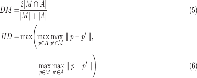where A is a set of points of RV boundary derived from automated segmentation, M is a set of points of RV boundary derived from manual segmentation. is the area of the automated segmentation, and is the area of the manual segmentation. is the Euclidean norm. HD can be defined as the largest minimum distance between the estimated RV contour and manual delineation.

D. Implementation Details

We performed experiments using Python and MATLAB R2015b on a DELL workstation with Intel(R) Core(TM) i7-7700 CPU@ 3.6GHz and 16 GB RAM. The graphics card is a NVIDIA Quadro K620, and the deep learning libraries were implemented with Keras (Theano).

III. Results

A. Cardiac MR Data

The collected cardiac MR image dataset includes 2900 images from 145 subjects. The subjects aged from 16 to 97 years old, with a mean of 58.9 years old. All of these subjects are selected from 3 hospitals affiliated with London Healthcare Center and St. Josephs HealthCare using scanners of 2 vendors (GE and Siemens). Each subject includes 20 frames across a cardiac circle. In each frame, the middle slice is selected following the standard AHA prescriptions [35] for validation of our proposed RegressionCNN. The pixel pitch of the MR images within small range (0.6836-2.0833 mm/pixel) with mode of 1.5625 mm/pixel. Two landmarks between the right ventricular wall and the left ventricular are manually labeled for each cardiac image to provide reference for cardiac ROI cropping. The cropped images are resized to dimension of . Two experienced cardiac radiologists check the manually obtained RV boundaries from all the cardiac MR images.

B. RV Segmentation Results

The estimated boundaries by our proposed RegressionCNN are measured using leave-one-subject-out cross validation. Fig.4 shows the segmentation results that the average DM and HD of each subject (20 images) and all subjects (2900 images). Despite of the challenges in segmenting RV from cardiac MR images, our proposed method achieves a high average DM of 0.8351, and a low average HD of 5.7613. Furthermore, the average DM of 117 subjects yield 0.8, which demonstrates that our proposed RegressionCNN can achieve accurate and robust RV segmentation from cardiac MR images. The great robustness of our method due to the seamless combination of CNN and regression segmentation model in a unified framework: (1) convolutional layers of CNN are able to learn high-level features containing global shape prior. Based on these robust features, the holistic regression model regresses all boundary points directly and simultaneously. This can naturally deal with local weak/no boundary and inhomogeneous intensity. (2) RegressionCNN regresses each boundary point to deal with the great diversity in RV boundaries. (3) RegressionCNN integrated RV feature extraction and regression model learning into one step. It reduces the latent mismatch influence between the feature extraction and following model learning to improve segmentation performance.

FIGURE 4.

RV segmentation results. (a) Average DM metric, each bar represents the average DM of one subject (20 images). The red line represents that the average DM of 145 subjects (2900 images) is 0.8351. (b) Average HD metric, each bar represents the average HD of one subject (20 images). The red line represents that the average HD of 145 subjects (2900 images) is 5.7613.

C. Correlation Analysis

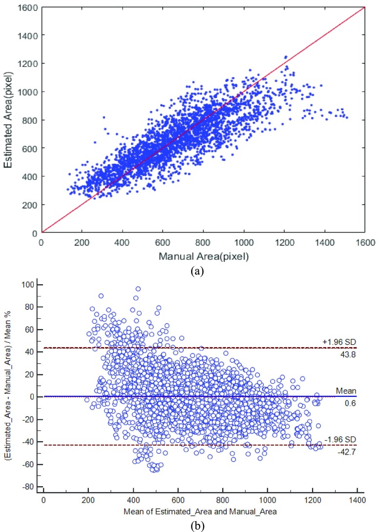
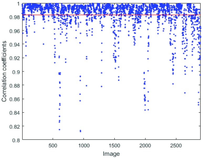
We use correlation analysis to demonstrate the high correlation between RegressionCNN’s segmentation results and the manual delineation. Fig. 5(a) shows the correlation between the estimated RV area and the manual delineation, most of the points around with red line, which illustrates estimated area of RV is closed to manual delineation. It also demonstrates the estimated area of RV is highly correlated to their manual delineation. Fig.5(b) reports the agreement between estimated area of RV and the manual delineation by using Bland-Altman [36]. The mean and confidence interval of the difference between the estimated and manual area were 0.6 and (−42.7 to 43.8). We can see that most points fall into the interval of the percentage difference between mean±1.96SD. It represents the 95% limits of agreement and demonstrates the estimated areas of RV highly agree with manual delineation. Fig.6 provides a qualitative visualization of the correlation coefficients of all images between the estimated RV boundary and the manual delineation. Most of correlation coefficients are higher than 0.98, and all the correlation coefficients are higher than 0.8. Hence, the estimated RV boundaries are highly consistent with their manual delineation. All of these demonstrate the great correlation between regressionCNN’s results and manual delineation.

FIGURE 5.

Correlation between the estimated RV area and the manual delineation. (a) correlation analysis. Points on the y=x line (red line) denote the complete overlapping, which can demonstrate great correlation between estimate result and manual delineation. (b) Agreement analysis of Bland-Altman. The level of agreement between the estimated area and manual area was represented by the interval of the percentage difference between mean±1.96SD.

FIGURE 6.

Boundary correlation coefficients of RegressionCNN’s segmentation result with all images. Each point shows the correlation coefficient between estimated RV boundary and manual delineation. The red line shows that the average correlation coefficient of 2900 images (145 subjects) is 0.9827.

D. Analysis of CNN Features

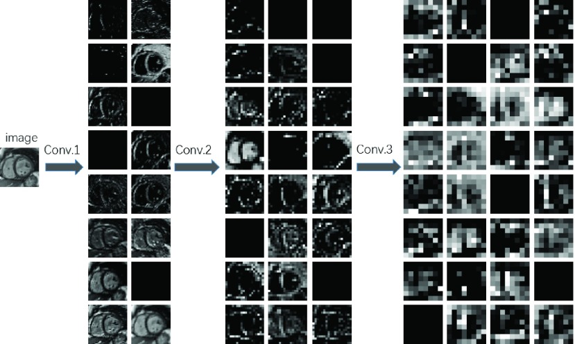
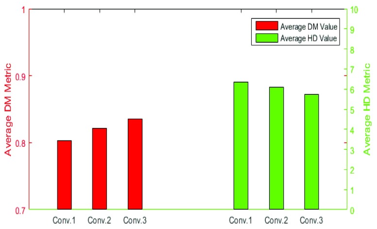
Segmentation performance would be improved if we can extract robust features from images. Our proposed RegressionCNN leverage the CNN to extract robust features from images to improve segmentation performance. CNN features are obtained by different convolutional kernels and could be regarded as the responses of image feature extractor. Besides, with the convolutional layers increase, feature maps are capable of providing more detailed information about images [37]. In the lower convolutional layers, they usually obtain shape information from RV. However, at a higher convolutional layer, the different feature maps from lower layers are merged into a common representation (one feature map) by a convolutional kernel. The feature maps of Higher convolutional layers have more information about the details and textures and learn higher-level RV representations (as shown in Fig.7). Moreover, the changes in details, such as scaling in input images, would have an influence on the feature maps of lower convolutional layers but not on the higher convolutional layers. This can reduce the noise’s interference and remain the invariability such as scale invariability. Hence, we only use the features from the last convolutional layer to train model and make a prediction. Indeed, we has demonstrated the last convolutional layer has better robust features by comparing estimated results using convolutional features from less convolutional layers. As shown in the Fig.8, the features obtained from deeper convolutional layer, the average DM value (red bar) is higher and the average HD value (green bar) is smaller. Therefore, the CNN features in last convolutional layer have better robustness to improve segmentation performance.

FIGURE 7.

Feature maps from different convolutional layers. Conv.x indicates the x-th convolutional layer.

FIGURE 8.

Comparison of the estimated results of RegressionCNN using the features from different convolutional layers. Conv.x represents the segmentation result using the features from x-th convolutional layer. Each red bar represents the DM value of RegressionCNN that using convolutional features of x-th convolutional layer to segment RV. Each green bar represents the HD value of RegressionCNN that using convolutional features of x-th convolutional layer to segment RV.

E. Analysis of Unified Segmentation Framework

To demonstrate our proposed RegressionCNN is able to reduce the potential mismatch influence between the feature extraction and following model learning by integrating feature extraction and model learning into one step. We separate convolutional feature extraction and regression model learning into two independent steps based on same regression segmentation model. As shown in Table 1, the results show that our proposed approach is superior to the regression segmentation of separated convolutional feature extraction and model learning (two-phase segmentation). Our proposed RegressionCNN has obtained higher average DM value. This success is derived from unified segmentation framework. Through integrating feature extraction and regression model learning into one step, RegressionCNN makes feature extraction be more specialized to better train RV segmentation model. It means that such seamless integration gives rise to an optimally convolutional feature extraction for accurately catching the features that are more relevant to RV segmentation task in training process. This can reduce the potential mismatch influence between the feature extraction and following model learning. Nevertheless, the two-phase segmentation loses the correlation between feature extraction and segmentation model learning.

TABLE 1. Comparison Between Our Approach and Other Segmentation Methods.

Method	Average DM	Average HD
RegressionCNN	0.8351 ± 0.0850	5.7613 ± 2.6286
Two-phase segmentation	0.8274 ± 0.0863	5.6192 ± 2.4040
Active Contour	0.8085 ± 0.0555	6.8284 ± 0.9801
Level Set	0.7749 ± 0.0693	7.1816 ± 1.0951
Graph Cut	0.7948 ± 0.1647	13.6855 ± 12.9129

F. Method Comparison

The performance of our proposed method can be further demonstrated by the comparison with some traditional segmentation methods. Table1 summarizes our segmentation results and compares it to previous segmentation methods including active contour [17], level set [18], graph cut [13]. Although these methods have achieved great success in many applications, the high complexities and variability of RV in cardiac MR images make these methods to meet great challenges. From Table 1, we can find that our proposed method outperforms these methods on the task of RV segmentation across all evaluation metrics. The results illustrate an advantage of our method over these methods: average DM improvements range from 0.0266 to 0.0602, and average HD improvements range from 1.1617 to 7.9242.

Fig. 9 visually gives a further illustration to demonstrate the good performance of RegressionCNN. We can visually find defects of these previous segmentation methods. As shown in Fig.9 (d), the active contour has a great challenge to segment RV with concave boundaries and local weak/no boundaries. Level set (as shown in Fig.9 (e)) may not converge to the RV boundary if the initialization is not close enough. And it is also sensitive to local weak/no boundaries. While the region intensity of RV is inhomogeneous. The results of graph cut (as shown in Fig.9 (f)) have many holes. Besides, if the neighboring structures to RV present similar photometric profiles. The ultimate segmentation results not only contain RV, but also include these similar structures. In comparison, our proposed regression segmentation (as shown in Fig.9(c)) is superior to these methods because of the following aspect: RegressionCNN relies on global shape prior to guide segmentation rather than boundary and intensity, which can naturally tackle local weak/no boundary and inhomogeneous. Besides, the complex variable shape of RV can be handled by regressing each point. Therefore, by combining the convolutional feature extraction and holistic regression model, RegressionCNN can better tackle complex variable shape, local weak/no boundary and inhomogeneous intensity simultaneously.

FIGURE 9.

Illustration of the difference in different RV segmentation performance. (a) 18 images with each row for local weak/no boundary, complex variable shape and inhomogeneous density of RV; (b) results of our proposed RegressionCNN; (c) results of active contours; (d) results of level set; (e) results of graph cuts. Each estimated segmentation is represented as a cyan contour. Each manual delineation is represented as a red contour.

IV. Discussion

In this paper, our aim is to segment RV from cardiac MR images accurately by integrating the holistic regression model and CNN into a unified framework. In previous studies, there has presented many effective methods for segmenting RV from cardiac images [5], [9], [10], [12], [14], [16], [19]. Our proposed RegressionCNN takes the RV segmentation as holistic boundary regression task, which is able to better tackle complex variable crescent shape, local weak/no boundary, inhomogeneous intensity of RV simultaneously. Besides, RegressionCNN combined convolutional features extraction and regression model learning into one step. It allows us to take full advantage of the convolutional features to directly guide RV segmentation of fully-connected layers.

Image feature extraction is the prerequisite for image segmentation. It is the most effective way to simplify the high-dimension image data. In our proposed RegressionCNN, we utilize multi-convolution layers to extract robust features [38]. Through convolutional operation and weight sharing, convolutional layers detect similar local information at different local area [29]. Therefore, convolutional layers can catch complex correlations at different local area, and give rise to detected global shape prior. These extracted global shape priors would be helpful in following holistic RV regression segmentation [21]. Fig.7 reports features extracted by different convolutional layers of our proposed RegressionCNN. It visually shows multiple convolutional kernels extracted multiple global shape priors in each convolutional layer. Besides, higher convolutional layers show more information about the details and textures and learn higher-level RV representations. Hence, compared with lower layers, the higher convolutional layers can extract more robust features to improve segmentation performance. Fig.8 reports last convolutional features indeed have best performance.

RegressionCNN takes the RV segmentation as boundary holistic regression task. We utilize the fully-connected layer as the holistic regression segmentation model. Because fully-connected layer provides the following advantages: (1) it has the ability to model a nonlinear mapping function from diverse cardiac MR images to desired RV boundaries. (2) It can easily achieve the multiple outputs by setting up the number of neurons of last fully-connected layer. Based on this, fully-connected layers can leverage strength of multi-output regression to estimate the RV boundary points simultaneously. This can fully consider the coupling among the points’ coordinates, than utilizing single-output regressor to regress coordinates one by one. (3) Fully-connected layer can naturally connect to convolutional layers. It can let us to combine the convolutional feature extraction and regression model learning in a unified framework (as shown in Fig.2).

The characteristic of regression determines that our RV is represented by many boundary points. There are also many advantages for this boundary representation: (1) due to RV is complex variable shape (as shown in Figure 1), it should be tackled by a flexible representation. Our boundary representation catches the diversity of RV boundaries to handle complex variable shape of RV by a few points (as shown in Fig.3). (2) Local weak/no boundary can be connected by points naturally (as shown in Fig.3). Based on these advantages. RegressionCNN is able to regress these points regardless of weak/no boundary or intensity, which poses a great challenge to previous segmentation methods. Table 1 reports that our segmentation results are superior to these previous segmentation methods. And Fig.9 visually demonstrates regression segmentation better tackles complex variable crescent shape, local weak/no boundary and inhomogeneous intensity of RV.

In our experiment, the most important part is a strong correlation between regression feature learning and our unified segmentation framework. Previous regression segmentation methods first always extract features of all training data [20]–[22]. It cannot establish a relationship between feature extraction and task models learning well. As a result, they cannot determine if the extracted features are the best features to segmentation model. Compared with these two-phase regression segmentation methods, our proposed regression segmentation approach can automatically extract relevant information from the cardiac MR images to learn a regression segmentation model in a unified segmentation framework. It is achieved by the seamless connection of CNN and holistic regression model. Such connection allows us to make full use of the Adam method to constantly optimize the convolutional layers to extract features. These features are correlated to RV regression segmentation task. Indeed, we showed that our proposed unified regression segmentation could better segment RV (as shown in Table 1).

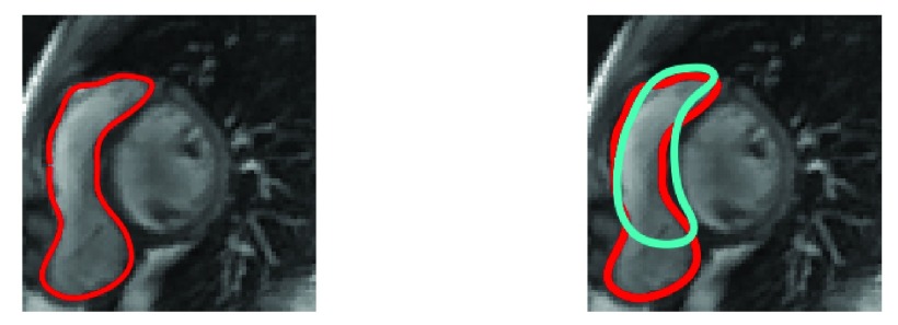
There are about 20 points which show not good correlations in the right upper corner in the Fig.5(a) illustrate the areas of manual delineations are larger than the estimated areas. These not good correlations are caused by about 20 images (one subject) (as shown in Fig.10). These RV shapes have very large deformation, which make RV have larger irregular shape. Due to the data limitations. Our method cannot learn this kind of RV shape well but rather to learn a not too big deformation, which can result in the smaller estimated area.

FIGURE 10.

Manual delineation (left). manual delineation(red line) vs estimated contour(cyan line) (right).

In the training process, according to the feedback of segmentation model, RegressionCNN constantly optimizes weights to learn the feature detector (convolutional layers) to train the segmentation model. It makes the feature detector variety to detect more detailed RV information from images to train the segentation model. While two-phase segmentation trains the segmentation model after extracting all the features of training images. It means the two-phase segmentation can not further learn detailed RV information to learn the segmentation model in the training process. Hence, compared with RegressionCNN, the features extracted by two-phase segmentation have less detailed and specific RV information, which have the better better generalized ability. This can result in that estimated RV shapes of two-phase segmentation are more consistent with the manual delineation. Due to HD is defined as the largest minimum distance between the estimated RV contour and manual delineation. And a smaller HD indicates a better match between predicted and manual segmentations. Therefore, the more generalized features of two-phase segmentation can reduce the overfitting of segmentation model to get the lower HD.

There are also limitations in our study, we ignore the relation between cardiac MR images across a cardiac circle. This may limit our proposed approach performance, and we will take this seriously in further research.

V. Conclusion

Segmenting RV from cardiac MR images accurately and automatically has a great clinical meaning for diagnosing cardiac diseases. Due to manual segmentation is tiresome and sensitive to intra- and inter-observer variability. Automated accurate RV segmentation approaches greatly meet needs of clinical applications. However, they face big challenges due to complex variable crescent shape, local weak/no boundaries and inhomogeneous intensity of RV. In this study, we formulate the RV segmentation as a boundary regression task. We proposed a regression segmentation approach called RegressionCNN, which based on a combination of CNN and holistic regression model to directly regress all boundary points of RV. RegressionCNN integrates feature extraction and regression model learning into one step. It can reduce the latent mismatch between the feature extraction and following regression model learning. Experiments was thoroughly validated on 2900 cardiac MR images acquired from 145 subjects, who are selected from 3 hospitals affiliated with London Healthcare Center and St. Josephs HealthCare. The results demonstrate that a good conformity between our estimated results and manual delineation by leave-one-subject-out cross validation. Therefore, our proposed RegressionCNN could be an effective way to segment RV from cardiac MR images accurately and automatically.

Funding Statement

This work was supported in part by the National Key Research and Development Program of China under Grant 2016YFC1300300, the Shenzhen Hong Kong Innovation Circle under Grant JCYJ20150401145529007, the National Science Foundation of China under Grant 61673020, the Provincial Natural Science Research Program of Higher Education Institutions of Anhui Province under Grant KJ2016A016, and the Anhui Provincial Natural Science Foundation under Grant 1708085QF143.

References

- [1].Mehta S. R.et al. , “Impact of right ventricular involvement on mortality and morbidity in patients with inferior myocardial infarction,” J. Amer. College Cardiol., vol. 37, pp. 37–43, Jan. 2001. [DOI] [PubMed] [Google Scholar]
- [2].Kevin L. G. and Barnard M., “Right ventricular failure,” Continuing Educ. Anaesthesia Crit. Care Pain, vol. 7, pp. 89–94, Jun. 2007. [Google Scholar]
- [3].Vitarelli A. and Terzano C., “Do we have two hearts? New insights in right ventricular function supported by myocardial imaging echocardiography,” Heart Failure Rev., vol. 15, pp. 39–61, Jan. 2010. [DOI] [PubMed] [Google Scholar]
- [4].Caudron J., Fares J., Vivier P.-H., Lefebvre V., Petitjean C., and Dacher J.-N., “Diagnostic accuracy and variability of three semi-quantitative methods for assessing right ventricular systolic function from cardiac MRI in patients with acquired heart disease,” Eur. Radiol., vol. 21, pp. 2111–2120, Oct. 2011. [DOI] [PMC free article] [PubMed] [Google Scholar]
- [5].Petitjean C.et al. , “Right ventricle segmentation from cardiac MRI: A collation study,” Med. Image Anal., vol. 19, pp. 187–202, Jan. 2015. [DOI] [PubMed] [Google Scholar]
- [6].Bonnemains L., Mandry D., Marie P.-Y., Micard E., Chen B., and Vuissoz P.-A., “Assessment of right ventricle volumes and function by cardiac MRI: Quantification of the regional and global interobserver variability,” Magn. Reson. Med., vol. 67, pp. 1740–1746, Jun. 2012. [DOI] [PubMed] [Google Scholar]
- [7].Petitjean C. and Dacher J.-N., “A review of segmentation methods in short axis cardiac MR images,” Med. Image Anal., vol. 15, no. 2, pp. 169–184, 2011. [DOI] [PubMed] [Google Scholar]
- [8].Zhuang X., “Challenges and methodologies of fully automatic whole heart segmentation: A review,” J. Healthcare Eng., vol. 4, pp. 371–407, Mar. 2013. [DOI] [PubMed] [Google Scholar]
- [9].Ringenberg J., Deo M., Devabhaktuni V., Berenfeld O., Boyers P., and Gold J., “Fast, accurate, and fully automatic segmentation of the right ventricle in short-axis cardiac MRI,” Comput. Med. Imag. Graph., vol. 38, pp. 190–201, Apr. 2014. [DOI] [PubMed] [Google Scholar]
- [10].Zhang H., Wahle A., Johnson R. K., Scholz T. D., and Sonka M., “4-D cardiac MR image analysis: Left and right ventricular morphology and function,” IEEE Trans. Med. Imag., vol. 29, no. 2, pp. 350–364, Feb. 2010. [DOI] [PMC free article] [PubMed] [Google Scholar]
- [11].Lorenzo-Valdés M., Sanchez-Ortiz G. I., Elkington A. G., Mohiaddin R. H., and Rueckert D., “Segmentation of 4D cardiac MR images using a probabilistic atlas and the EM algorithm,” Med. Image Anal., vol. 8, pp. 255–265, Sep. 2004. [DOI] [PubMed] [Google Scholar]
- [12].Bai W., Shi W., Wang H., Peters N. S., and Rueckert D., “Multi-atlas based segmentation with local label fusion for right ventricle MR images,” Image, vol. 6, p. 9, Jan. 2012. [Google Scholar]
- [13].Boykov Y., Veksler O., and Zabih R., “Fast approximate energy minimization via graph cuts,” IEEE Trans. Pattern Anal. Mach. Intell., vol. 23, no. 11, pp. 1222–1239, Nov. 2001. [Google Scholar]
- [14].Grosgeorge D., Petitjean C., Dacher J.-N., and Ruan S., “Graph cut segmentation with a statistical shape model in cardiac MRI,” Comput. Vis. Image Understand., vol. 117, no. 9, pp. 1027–1035, 2013. [Google Scholar]
- [15].Maier O. M. O., Jiménez D., Santos A., and Ledesma-Carbayo M. J., “Segmentation of RV in 4D cardiac MR volumes using region-merging graph cuts,” in Proc. Comput. Cardiol., Sep. 2012, pp. 697–700. [Google Scholar]
- [16].Avendi M. R., Kheradvar A., and Jafarkhani H., “Automatic segmentation of the right ventricle from cardiac MRI using a learning-based approach,” Magn. Reson. Med., vol. 78, no. 6, pp. 2439–2448, 2017. [DOI] [PubMed] [Google Scholar]
- [17].Kass M., Witkin A., and Terzopoulos D., “Snakes: Active contour models,” Int. J. Comput. Vis., vol. 1, no. 4, pp. 321–331, 1988. [Google Scholar]
- [18].Li C., Xu C., Gui C., and Fox M. D., “Distance regularized level set evolution and its application to image segmentation,” IEEE Trans. Image Process., vol. 19, no. 12, pp. 3243–3254, Dec. 2010. [DOI] [PubMed] [Google Scholar]
- [19].Qin X., Cong Z., Halig L. V., and Fei B., “Automatic segmentation of right ventricle on ultrasound images using sparse matrix transform and level set,” Proc. SPIE, vol. 58, p. 21, Mar. 2013. [DOI] [PMC free article] [PubMed] [Google Scholar]
- [20].Wang Z., Zhen X., Tay K., Osman S., Romano W., and Li S., “Regression segmentation for M3 spinal images,” IEEE Trans. Med. Imag., vol. 34, no. 9, pp. 1640–1648, Aug. 2015. [DOI] [PubMed] [Google Scholar]
- [21].Zhen X., Yin Y., Bhaduri M., Nachum I. B., Laidley D., and Li S., “Multi-task shape regression for medical image segmentation,” in Proc. Int. Conf. Med. Image Comput. Comput., Assist. Intervent., 2016, pp. 210–218. [Google Scholar]
- [22].He X., Lum A., Sharma M., Brahm G., Mercado A., and Li S., “Automated segmentation and area estimation of neural foramina with boundary regression model,” Pattern Recognit., vol. 63, pp. 625–641, Mar. 2017. [Google Scholar]
- [23].Tuia D., Verrelst J., Alonso L., Perez-Cruz F., and Camps-Valls G., “Multioutput support vector regression for remote sensing biophysical parameter estimation,” IEEE Geosci. Remote Sens. Lett., vol. 8, no. 4, pp. 804–808, Jul. 2011. [Google Scholar]
- [24].Xiong T., Bao Y., and Hu Z., “Multiple-output support vector regression with a firefly algorithm for interval-valued stock price index forecasting,” Knowl.-Based Syst., vol. 55, pp. 87–100, Jan. 2014. [Google Scholar]
- [25].Osowski S., Siwek K., and Markiewicz T., “MLP and SVM networks—A comparative study,” in Proc. Signal Process. Symp. (NORSIG), 2004, pp. 37–40. [Google Scholar]
- [26].Brébisson A. D. and Montana G., “Deep neural networks for anatomical brain segmentation,” in Proc. IEEE Conf. Comput. Vis. Pattern Recognit. Workshops, Jun. 2015, pp. 20–28. [Google Scholar]
- [27].Moeskops P., Viergever M. A., Mendrik A. M., de Vries L. S., Benders M. J. N. L., and Išgum I., “Automatic segmentation of MR brain images with a convolutional neural network,” IEEE Trans. Med. Imag., vol. 35, no. 5, pp. 1252–1261, May 2016. [DOI] [PubMed] [Google Scholar]
- [28].Tran P. V. (2016). “A fully convolutional neural network for cardiac segmentation in short-axis MRI.” [Online]. Available: https://arxiv.org/abs/1604.00494 [Google Scholar]
- [29].Litjens G.et al. , “A survey on deep learning in medical image analysis,” Med. Image Anal., vol. 42, no. 9, pp. 60–88, Dec. 2017. [DOI] [PubMed] [Google Scholar]
- [30].Glorot X., Bordes A., and Bengio Y., “Deep sparse rectifier neural networks,” in Proc. Int. Conf. Artif. Intell. Stat., 2011, pp. 315–323. [Google Scholar]
- [31].Hinton G. E., Srivastava N., Krizhevsky A., Sutskever I., and Salakhutdinov R. R., “Improving neural networks by preventing co-adaptation of feature detectors,” Comput. Sci., vol. 3, no. 4, pp. 212–223, 2012. [Google Scholar]
- [32].Kingma D. P. and Ba J. (2014). “Adam: A method for stochastic optimization.” [Online]. Available: https://arxiv.org/abs/1412.6980 [Google Scholar]
- [33].Zijdenbos A. P., Dawant B. M., Margolin R. A., and Palmer A. C., “Morphometric analysis of white matter lesions in MR images: Method and validation,” IEEE Trans. Med. Imag., vol. 13, no. 4, pp. 716–724, Dec. 1994. [DOI] [PubMed] [Google Scholar]
- [34].Huttenlocher D. P., Klanderman G. A., and Rucklidge W. J., “Comparing images using the Hausdorff distance,” IEEE Trans. Pattern Anal. Mach. Intell., vol. 15, no. 9, pp. 850–863, Sep. 1993. [Google Scholar]
- [35].Cerqueira M. D.et al. , “Standardized myocardial segmentation and nomenclature for tomographic imaging of the heart: A statement for healthcare professionals from the cardiac imaging committee of the council on clinical cardiology of the American Heart Association,” J. Nucl. Cardiol., vol. 105, pp. 539–542, Jan. 2002. [DOI] [PubMed] [Google Scholar]
- [36].Bland J. M. and Altman D. G., “Measuring agreement in method comparison studies,” Stat. Methods Med. Res., vol. 8, no. 2, pp. 135–160, 1999. [DOI] [PubMed] [Google Scholar]
- [37].Zeiler M. D. and Fergus R., “Visualizing and understanding convolutional networks,” in Proc. Eur. Conf. Comput. Vis., 2014, pp. 818–833. [Google Scholar]
- [38].Razavian A. S., Azizpour H., Sullivan J., and Carlsson S., “CNN features off-the-shelf: An astounding baseline for recognition,” in Proc. IEEE Conf. Comput. Vis. Pattern Recognit. Workshops, Jun. 2014, pp. 512–519. [Google Scholar]