QSAR modeling for predicting reproductive toxicity of chemicals in rats for regulatory purposes

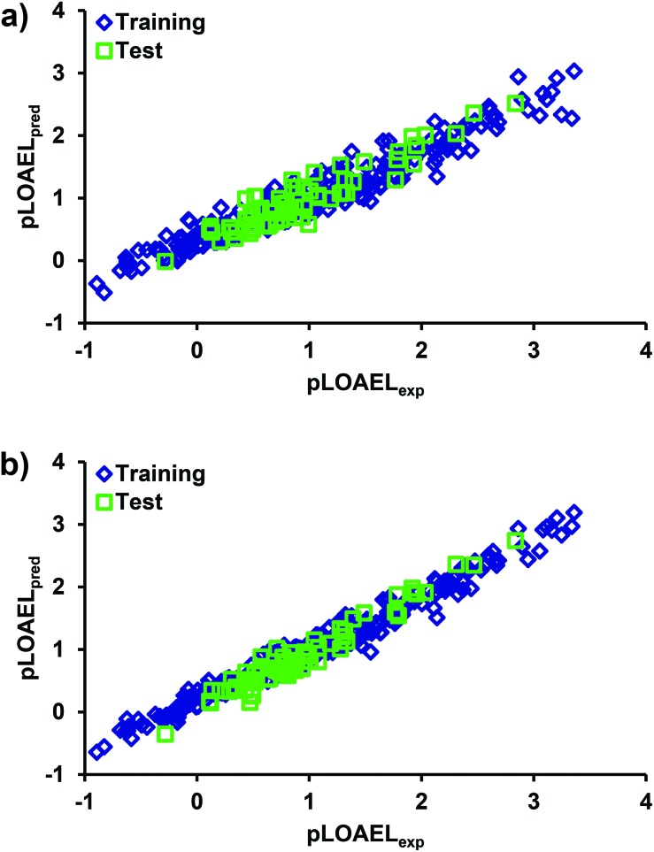
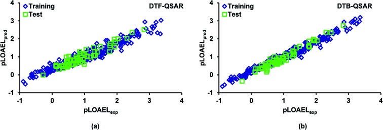
The figure shows the prediction performance of (a) DTF-QSAR and (b) DTB-QSAR models for pLOAEL (rat) in training and test data.

Abstract

The experimental determination of multi-generation reproductive toxicity of chemicals involves high costs and a large number of animal studies over a long period of time. Computational toxicology offers possibilities to overcome such difficulties. In this study, we have established ensemble machine learning (EML) based quantitative structure–activity relationship models for predicting the reproductive toxicity potential (LOAEL) of structurally diverse chemicals in accordance with the OECD guidelines. Accordingly, decision tree forest (DTF) and decision tree boost (DTB) QSAR models were developed using a novel dataset composed of the toxicity endpoints for 334 chemicals. Relevant structural features of chemicals responsible for toxicity potential were identified and used in QSAR modeling. The generalization and prediction abilities of the constructed QSAR models were evaluated by internal and external validation procedures and by deriving several stringent statistical criteria parameters. In the test set, the two models (DTF and DTB) yielded R² of 0.856 and 0.945, between the experimental and predicted endpoint toxicity values. The models were also evaluated for predictive use through the most recent criteria based on root mean squared error (RMSE) and mean absolute error (MAE). The values of various statistical validation coefficients derived for the test data were above their respective threshold limits and thus put a high confidence in this analysis. The applicability domains of the constructed QSAR models were defined using the leverage and standardization approaches. The results suggest that the proposed QSAR models can reliably predict the reproductive toxicity potential of diverse chemicals and can be useful tools for screening new chemicals for safety assessment.

1. Introduction

Humans are exposed to a variety of chemicals willingly through the intake of drugs and pharmaceuticals, food products, beverages etc., and unwillingly due to interactions with environmental chemicals and adulterants in various consumables. Exposure to many of these chemicals has been established to cause several toxic and adverse health effects, including reproductive toxicity in animals. Reproductive toxicity refers to adverse effects produced by a chemical on the reproductive ability of individuals such as alteration of sexual organs and behavior, and the development of toxicity in offspring.1 The results of animal studies are used by regulatory agencies to help set human exposure guidelines.2 The primary study used for assessing reproductive effects of chemicals is the multi-generation reproductive test,3,4 which is typically conducted under continuous exposure of male and female rats from 10 week premating through lactation in the second generation.5 The multi-generation study also provides information about the effects of the test substance on neonatal morbidity, mortality, and test organs in the offspring, and data on prenatal and post-natal developmental toxicity.6 The LOAEL (lowest observed adverse effect level) dose of a chemical is considered an appropriate endpoint in multi-generation reproductive toxicity studies. The LOAEL is the minimum dose of a chemical for which any adverse effect is observed. The USEPA and OECD have developed experimental protocols for determining the reproductive toxicity potential of chemicals in test animals3,4,7,8 and the EPA's toxicity reference database has been developed for animal based multi-generation reproduction toxicity studies in rats, mice, hamsters, and minks (ToxRefDB)9 and specific effects within this category include reproductive performance measures, male and female reproductive tract effects, and sexual development landmarks. However, the multi-generation reproductive toxicity tests are the costliest and require a large number of animals. Moreover, for a large number of chemicals in use and newly added ones, it is almost impossible to screen them for their reproductive toxicity potential assessment using the experimental protocols.6 Accordingly, attention has been focused on finding in vitro alternatives that can effectively screen a large number of compounds for their effects relevant to reproductive toxicity.5 Recently, the European Union REACH (Registration, Evaluation, Authorization and Restriction of Chemicals) legislation has emphasized toxicological hazard and risk assessments for all new and existing chemicals10 and advocates the use of sufficiently validated computational prediction models based on QSAR (quantitative structure–activity relationship) to fill in the toxicity data gaps, and thus save time, and money and help reduce the numbers of animals used for experimental testing purposes.11 QSAR uses chemical information on compound structures in the form of numerical quantities (molecular descriptors) to correlate with the response property or toxicity using appropriate statistical tools.12 Recently, Dearden13 has summarized the history and development of QSARs. The OECD (Organization for Economic Cooperation and Development) has provided guidelines for QSAR model development and validation for regulatory purposes.14 The OECD guidelines emphasize the selection of a definite dataset with a defined end-point (principle 1), an explainable model building strategy in view of the nature of the selected data (principle 2), a defined applicability domain of the constructed model (principle 3), appropriate validation strategies corresponding to the goodness of fit, robustness and predictivity (principle 4), and finally offering a possible mechanistic interpretation of the developed models (principle 5). Therefore, robust and reliable QSAR models based on an appropriate method and validated through OECD recommended procedures are required for the screening of chemicals for their reproductive toxicity potential (LOAEL) for their risk assessment. However, predictive modeling of chemical toxicity requires high-quality experimental toxicity data for the development and validation of new computational approaches. Subsequently, in the past, significantly less attention has been paid to the development of predictive QSAR models for chemical-induced reproductive toxicity endpoints. The EPA's Toxicity Reference Database (ToxRefDB), which compiles toxicity data from high quality experimental studies, provides opportunities for QSAR modelling studies.15 Subsequently, a few studies have reported (Q)SAR analyses of reproductive toxicity data.1,5,16,17 However, these were limited to classification models only and no attempt has been made to perform regression QSAR analysis for reproductive toxicity prediction.

In recent years, ensemble machine learning (EML) methods, such as the decision tree forest (DTF) and the decision tree boost (DTB), have emerged as unbiased tools for QSAR modelling in computational toxicology. Ensemble techniques have the advantage of alleviating the small sample size problem by averaging and incorporating over multiple models to reduce the potential for over-fitting the training data.18,19 These techniques are inherently non-parametric statistical methods and make no assumption regarding the underlying distribution of the values of predictor variables and can handle numerical data that are highly skewed or multi-model in nature20 and, moreover, are capable of capturing the nonlinear dependence in data and have been successfully used for QSAR studies.21–29

The present study aims to identify relevant structural features of the chemicals that could be responsible for their reproductive toxicity potential in rats; and to establish reliable QSAR models strictly in accordance with the OECD guidelines, using the ToxRefDB toxicity data. Accordingly, QSAR models based on EML methods (DTF and DTB) were constructed. The models were rigorously validated using stringent statistical parameters to ensure their external predictivity for untested new chemicals.

2. Materials and methods

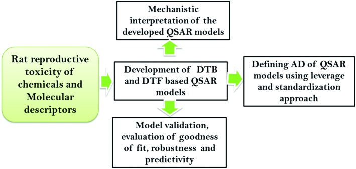
In this study, we intend to develop QSAR models for screening the chemicals for their reproductive toxicity potential (LOAEL) in rats using EML methods (DTF and DTB), in accordance with the OECD principles. A schematic diagram showing the modeling steps is presented in Fig. 1.

Fig. 1. A workflow diagram showing the QSAR modeling steps.

2.1. The dataset

Multi-generation reproductive toxicity data (oral LOAEL dose, mg per kg body weight per d) of chemicals in rats were collected from the ToxRefDB.9 This database contained multi-generation reproductive toxicity endpoints of 863 compounds in rats with the LOAEL dose, which have been generated according to the OPPTS guideline (870.38).3 According to Martin et al.5 the reproductive toxicity effects investigated were the reproductive performance measures (e.g., fertility, mating, and gestational interval), male and female reproductive tract effects (e.g., testis, epididymis, ovary, and uterus pathology and weight, along with sperm measures and morphology), and sexual development landmarks (e.g., preputial separation, vaginal opening, and anogenital distance). Additional information regarding the treatment groups, including the life stage and generation of the animals and the administered dose, was available in ToxRefDB to provide additional context for each chemical's reproductive toxicity potential. In order to obtain a high quality dataset, a rigorous screening process was applied here. All the mixtures, duplicates and salts were removed. Finally, a total of 334 chemicals in rats were retained for QSAR analysis, which included 306 pesticides, 14 pharmaceuticals and 14 other organic chemicals (Table S1, ESI†). Among the toxicity endpoints, 4 studies referred to a single generation, 299 to two generations, 30 to three generations and a single study to four generations, respectively. Prior to the QSAR analysis, the LOAEL values were converted into the negative logarithmic scale (pLOAEL, mmol per kg bw per d). The end-point toxicity (pLOAEL) values ranged between –0.89 and 3.36.

2.2. The molecular descriptors

In total, 633 1D and 2D molecular descriptors were calculated for all the compounds using Chemopy.30 For calculating the descriptors, SMILES (simplified molecular input line entry system) of the compound were obtained from ChemSpider.31 The chemical structures available in ChemSpider corresponding to the SMILES of the considered molecules were compared with those in the PubChem.32 For the compounds for which the chemical structures were found different, the SMILES of such molecules were taken from the PubChem for descriptor calculations. The calculated descriptors belong to the constitutional, autocorrelation, Basak, Charge, MOE-type, Burden, connectivity, E-state, Kappa, molecular property, and topological categories. Although, during the development of the models, all the descriptors in the pool were used in order to identify the most relevant features, in the final QSAR models the descriptors that can demonstrate the physical meaning of the structural attributes of molecules were retained to ensure the compliance of the OECD principles.

2.3. Data processing and descriptor selection

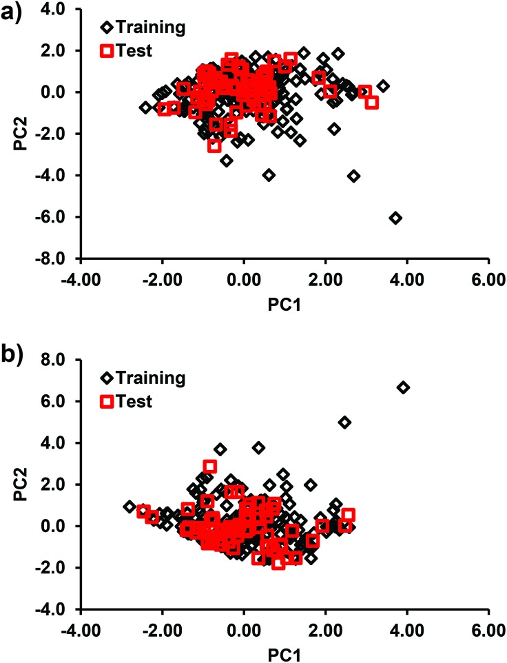
For QSAR analysis, the reproductive toxicity data (rat) were split into the training (80%) and test (20%) sets using the random distribution approach. A random distribution ensures a uniform selection of test set molecules that cover the entire range of the activity space of the total data.33 Further, the distribution of the structural features of the test and training set compounds was checked using the principal components analysis (PCA)34 scores (Fig. 2). From these plots, it is evident that the test set compounds were located in close proximity to the training set compounds.

Fig. 2. Plot showing the distribution of the PCA scores of the descriptors in the training and test compounds in (a) DTF QSAR and (b) DTB QSAR analyses.

For the selection of relevant features for QSAR model development, descriptors with low variation (≤0.5) were excluded from the pool. With the remaining descriptors, DTF and DTB based QSAR models were constructed using the training data performing repeated runs and excluding the least contributing.21 Optimal model parameters were then determined through a 10-fold cross-validation (CV). The mean squared error (MSE) values were calculated to rank the contribution of the descriptors in the current set for each model. The lowest ranked descriptors (<10% contribution) were then removed in the successive modeling steps.22 The most significant descriptors were then retained and the corresponding prediction accuracies were computed. Finally the descriptors retained for the QSAR models (DTF, DTB) are presented in Table 1. The distribution (range) of the selected descriptors for QSAR analysis shows that the compounds used in this study covered a sufficiently large structural space.

Table 1. Selected descriptors in QSAR modeling.

Descriptor symbol	QSAR model	Descriptor range	Description
naccr	DTF	0.00–14.00	Number of H-bond acceptors
S35	DTF	0.00–70.15	Sum of E-state of atom type: dO
S36	DTF, DTB	0.00–63.67	Sum of E-state of atom type: ssO
Smax	DTF, DTB	2.23–15.07	The maximal E-state value in all atoms
Smin	DTF, DTB	[–5.71]–1.59	The minimal E-state value in all atoms
TPSA	DTB, DTF	0.00–221.31	Topological polarity surface area

The Tanimoto similarity index (TSI) was calculated to evaluate the structural diversity of the compounds considered for QSAR modeling.35 TSI provides a measure for identifying the mechanistic groups the target chemical was most likely to belong to.36 The TSI for a pair of molecules, A and B, was calculated as: TSI_AB = 2Z_AB[Z_AA + Z_BB – Z_AB]^–1, where Z is the similarity matrix. The TSI ranges from 0 (no similarity) to 1 (pair-wise similarity). Smaller TSI means that compounds have good diversity. The TSI values of the considered compounds ranged between 0.001 and 0.229, which suggests a sufficiently high structural diversity among the considered compounds.

2.4. The QSAR model development

In this study, the QSAR models were developed using the EML methods (DTF and DTB) for predicting the reproductive toxicity (LOAEL) of the organic chemicals in rats. In the EML approach, multiple learners are trained to solve the same problem. An ensemble contains a number of base learners.37 The generalization ability of an ensemble is usually much stronger than that of the base learners. Ensemble learning is able to boost weak learners to make accurate predictions. The DTF38 and DTB39 are ensembles of SDTs (single decision trees). The DTF method implements the bagging algorithm, which derives bootstrapped replicas of the original data. A bootstrapped sample is constructed40 as 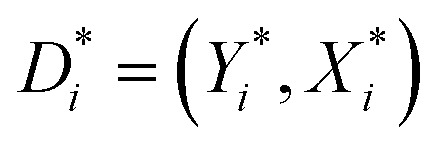, where D consists of data {(X_i, Y_i), i = 1, 2, …, n}, Y_i is the real-valued response and X_i is a p-dimensional predictor variable for the i^th instance. A bootstrapped predictor E(YIX = x) = f(x) is then estimated as , where C_n(x) = h_n(D₁, …, D_n)(x), and h_n is the n^th hypothesis. Finally, the bagged predictor is given as . The bagging technique uses the out of bag data rows for model validation and can reduce variance when combined with the base learner generation, with a good performance.

The stochastic gradient boosting algorithm implemented in the DTB method creates a tree ensemble, as F_m(x) = F_m–1(x) + Tree_m(x), where F_m represents the sum of all trees built in the model. The method minimizes the loss function in the training set, {x,y}, where x and y are predictor and response variables, respectively. Regardless of the loss-function, the trees fitting the gradient on pseudo-residuals are regression trees trained to minimize MSE. The regularization parameter is the number of gradient boosting iterations and achieved by shrinkage, which consists in modifying the update rule as: F_m(x) = F_m–1(x) + υγ_mh_m(x), 0 < υ ≤ 1, where υ is the learning rate, and h_m(x) is the base learner. In this method, a certain tree population is selected and the first tree is fitted to the data. The residuals from the first tree are then fed into the second tree which attempts to reduce the error. This process is repeated through a chain of successive trees and the final predicted value is formed by adding the weighted contribution of each tree.39 The number and depth of trees are the method's parameters in both the DTF and DTB. However, the primary disadvantage of DTF and DTB is that the models are complex and cannot be visualized like a single tree.

2.5. Model validation metrics

The DTF and DTB QSAR models developed here were validated by both the internal and the external validation procedures. For internal validation, a 10-fold CV procedure was adopted. In CV, the training data D are divided into k (= 10) non-overlapping subsets, D₁, D₂, …, D_k. At each iteration i (i = 1 to k), the model is trained with D – D_i and tested on D_i. In this approach, each test set is independent of the others.41 The optimal architectures of the models were selected on the basis of the MSE in the training and validation data42 calculated as: , where n is the number of data points, and ŷ_i and y_i are the model predicted and measured values of the response variable, respectively. For the external validation, a separate test set was used, which was kept out during the training phase. The prediction accuracies of the developed QSAR models were evaluated in terms of the statistical parameters derived for the test data, such as the R² (squared correlation coefficient) and the root mean squared error (RMSE). Recently, Alexander et al.43 emphasized that the prediction accuracy of a QSAR model can be adequately assessed using the R² and RMSE values in the test data and proposed corresponding criteria, R² > 0.6 for the test set, calculated as: 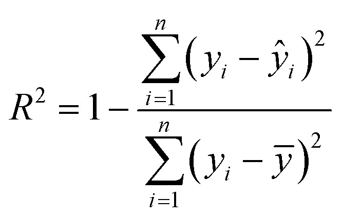, where y_i and ŷ_i have their usual meanings and ȳ is the mean of the measured value of the variable. Moreover, the test set RMSE of less than 10% of the range of the target property is considered to be adequate. The prediction quality of the developed QSAR models for test data was also assessed using the recently proposed mean absolute error (MAE) criteria.44 The MAE is considered to be a simpler and more straightforward determinant of prediction errors45 and is calculated as: . For a good prediction, a QSAR model should meet the following criterion: MAE ≤ 0.1 × training set range AND MAE + 3σ ≤ 0.2 × training set range, whereas a model will be considered to be a bad predictor if MAE > 0.15 × training set range OR MAE + 3σ > 0.25 × training set range. Here, the σ value denotes the standard deviation of the absolute values for the test set data. The predictions which do not fall under either of the above two conditions may be considered to be of moderate quality. The Y-scrambling test was performed to check for any chance-correlation in the developed QSAR models.46 Accordingly, models were derived using various randomly rearranged endpoint activities in the training data with the selected descriptors and these were compared with the optimal models in terms of the corresponding values of R². The chance-correlation in the developed QSAR models was also checked deriving the value of ^cR_p² for the scrambled models47 as: where R_r² represents the squared mean correlation coefficient of the randomized model. A model for which the ^cR_p² exceeds 0.5 might be considered not the outcome of mere chance only.

2.6. Applicability domain analysis

The applicability domains (AD) of the developed QSAR models were defined using the leverage48 and standardization49 approaches. The AD of a predictive model defines the theoretical region in space within which a model can make reliable predictions.50,51 In the leverage method, the distance of a compound from the centroids of its training set is measured by the leverage, h_i, of the compound, calculated from the descriptor matrix (X) as: h_i = x_i^T(X^TX)^–1x_i, where x_i is a raw vector of molecular descriptors for the i^th compound. A value of h_i > h* indicates that the structure of the compound substantially differs from those used for the model calibration. The h* value is given as:52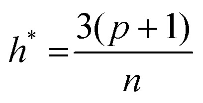, where p is the number of variables used in the model, and n is the number of training compounds. However, a major limitation of this method is that the value of h*, hence, the number of compounds within or outside the AD of a model, would depend on the number of compounds (n) in the training data. The AD of the QSAR models was also analyzed by the standardization approach,49 which identifies the X-outliers (in the training set) and the compounds that reside outside the AD (in the test set). In this approach, the standardized value of each descriptor for each compound in the training and test data is calculated as 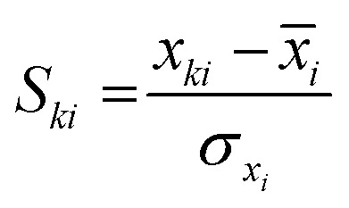, where k = 1 to n (n is the total number of compounds), i = 1 to m (m is the number of descriptors), S_ki is the standardized descriptor i for compound k (from the training or test set), x_ki is the original descriptor i for compound k (from the training or test set), x[combining macron]_i is the mean value of the descriptor x_i for the training set compound only, and σ_xi is the standard deviation of the descriptor x_i for the training set compounds only. If the maximum standardized values, [S_i]_max(k), for the compounds are less than 3, there is no X-outlier in the training set and no compound outside the AD in the test set; however, in case the [S_i]_max(k) for any compound exceeds 3, the minimum standardized value [S_i]_min(k) is calculated and if [S_i]_min(k) for a compound exceeds 3, the compound is an X-outlier (if in the training set) and is outside AD (if in the test set). In case a compound has [S_i]_max(k) > 3 and [S_i]_min(k) < 3, then S_new(k) can be calculated as S_new(k) = S[combining macron]_k + 1.28σ_Sk, where S[combining macron]_k and σ_Sk are the mean and standard deviation of S_i(k) values of the compound k, respectively. If for a compound, S_new(k) ≤ 3, then the compound is not an X-outlier (if in the training) and is within AD (if in the test set).

3. Results and discussion

3.1. QSAR model development and validation

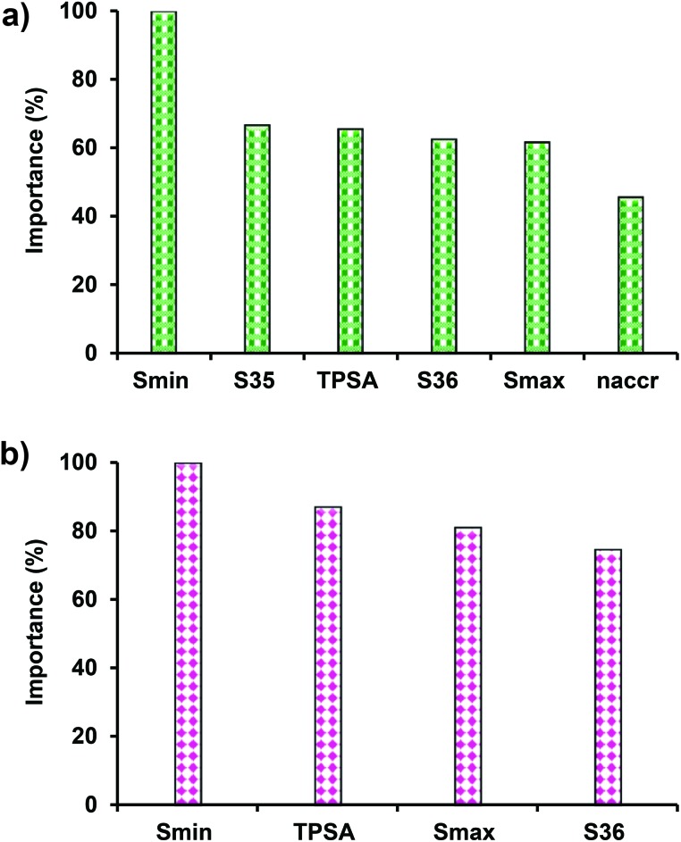
EML based QSAR models (DTF and DTB) were developed with an aim to predict the reproductive toxicity potential (LOAEL) of diverse chemicals in rats in accordance with the OECD principles. The two approaches (DTF and DTB) identified six (S35, S36, Smin, Smax, naccr, and TPSA) and four (S36, Smin, Smax, and TPSA) descriptors, respectively, with four descriptors common in both models. The optimal DTF and DTB models have 200 and 410 number of trees in series, 25 and 10 maximum depth of any tree, and 161.5 and 803.8 number of average group splits, respectively. In the training and 10-fold CV, the MSE values for DTF and DTB models were 0.11, 0.59 and 0.05, 0.60, respectively. In Y-randomization, the respective values of R² and ^cR_p² for these QSAR models derived through 10-fold CV were 0.009, 0.929 and 0.010, 0.965, which revealed that the original models are unlikely to arise as a result of chance-correlation. Moreover, according to Topliss53 to minimize the chance correlation in regression methods, the ratio of training set compounds to the descriptors should be at least 5 : 1.54 In the present study the ratio between the training set compounds (n = 267) and selected descriptors (6 in DTF and 4 in DTB) was much higher in the two QSAR models. The constructed models in the training and test data captured 87.71%, 85.65% (DTF), and 94.82%, 94.49% (DTB), respectively, of the data variances. The proportion of variance explained by model variables is the best single measure of how well the predicted values match the actual values. A model predicting exactly matching values with measured ones would explain 100% variance in data.19 The contributions of different descriptors in the two models are plotted in Fig. 3. In DTB, the relative importance of each independent variable to the model fit is measured through a reduction in the Huber loss summed across all the internal nodes, of all the trees, that split on that variable and divided by the total number of internal nodes (number of internal nodes per tree × number of trees), yielding a squared importance for that variable. In DTF, the contribution measures are based on the number of times a variable is selected for splitting, weighted by the squared improvement to the model as a result of each split, and averaged over all the trees.55 The relative importance is finally obtained in the range of 0–100 percent.56

Fig. 3. Plot showing the contribution of input descriptors in (a) DTF QSAR and (b) DTB QSAR models.

Fig. 3 shows that in both the DTF and DTB models, Smin has the highest (100%) contribution, whereas naccr (45.61%) in DTF and S36 (74.65%) in DTB contributed the least among the selected descriptors. The S35, S36, Smax, and Smin are the E-state (electrotopological state index) descriptors. The E-state index is developed from chemical graph theory and uses the chemical graph (hydrogen-suppressed skeleton) for the generation of atom-level structure indices. The index is based on the electronic effect of each atom on the other atoms in the molecule as modified by molecular topology.57 It provides information on the electronic state of the atom which depends on π-bonds, lone pair electrons and σ-bonds that reflect quantitative availability of valence electrons.58 The S35 and S36 descriptors represent the sum of E-state of atom type O and –O–, respectively. The Smax and Smin represent the maximum and minimum E-state values in all atoms. The topological polar surface area (TPSA) is defined as the part of the surface area of the molecule associated with N, O, and S and H-bonded to any of these atoms.59 It correlates well with the passive molecular transport through membranes and allows the prediction of the transport properties of chemicals.60 The naccr is a constitutional descriptor, and represents the number of H-bond acceptors in a molecule. The molecular descriptors used in the models encode information about the structure, branching, electronic effects and polarity of the molecules, and thus implicitly account for the cooperative effect between functional groups. Among these, the naccr (r = 0.08) and S36 (r = 0.20) have a positive correlation with the endpoint (pLOAEL), whereas S35 (r = –0.14), Smax (r = –0.05), Smin (r = –0.23), and TPSA (r = –0.15) exhibited a negative relationship with the endpoint toxicity. A positive relationship between a descriptor and the endpoint toxicity (pLOAEL) suggests that a higher value of the descriptor for a chemical would mean an enhanced toxicity potential, whereas a negative relationship would reflect a lower toxicity endpoint.

The external predictivity of the developed QSAR models was evaluated using the R² and RMSE values in the training and test data (Table 2). The R² represents the percentage of variability that can be explained by the model and RMSE describes an average measure of error in predicting the dependent variable.19 The R² values obtained by these models (DTF and DTB) in the training and test sets were 0.877, 0.948 and 0.856, 0.945, respectively. These values are higher than the respective threshold values prescribed for the training (0.50) and test (0.60) arrays.43,61 Identical values for the R² in training and test sets indicate that the test set selected for the QSAR model development had a similar distribution of responses to the training set. The RMSE values yielded by the two models in training and test data were 0.33, 0.23 (DTF) and 0.21, 0.14 (DTB), respectively (Table 2). According to a recent criterion proposed by Alexander et al.43 a QSAR model may be considered useful if the RMSE in test data is less than 10% of the test data range. In this study, the test data range was 3.12 and the RMSE values yielded by the two models in the test set were less than 0.31, and hence the developed QSAR models will be useful for future predictions of new compounds. The external predictivity of the developed QSAR models was also tested using the MAE based criteria recently proposed by Roy et al.44 According to this criterion, the performance of a QSAR model will be ‘good’, if the MAE in the test data is less than 10% of the training data range (0.10 × TR). From the results (Table 2), it is evident that the MAE values yielded by DTF and DTB models in test data were 0.18 and 0.11, respectively. These values are less than 10% of the training data range (TR = 4.25), thus validating the goodness of the developed QSAR models for external prediction. These criteria parameter values demonstrated the high predictive power of the constructed QSAR models for external prediction.

Table 2. Performance parameters for the QSAR models.

QSAR models	Data set	R 2	RMSE	Data set range	MAE	TR a × 0.1	MAE + 3σ	TR a × 0.2
DTF	Training	0.877	0.33	4.25	—	—	—	—
	Test	0.856	0.23	3.12	0.18	0.43	0.59	0.85
DTB	Training	0.948	0.21	4.25	—	—	—	—
	Test	0.945	0.14	3.12	0.11	0.43	0.36	0.85

^aTR training set range.

A distribution plot of experimental and model predicted values of the response variable in training and test arrays may provide a good measure of the model predictivity. It also helps to visualize any under- or over-estimation of the endpoint variable throughout the domain. The experimental and predicted values of the pLOAEL values for the considered chemicals in the training and test data are plotted in Fig. 4. It is evident that the predicted results for both the QSAR models are in good agreement with the corresponding experimental values both in training and test sets. A further analysis of the predicted results revealed that 97% of the predicted pLOAEL values (DTF QSAR) in the test set were within 0.5 units, whereas in DTB QSAR, none of the predicted values showed deviation >0.5 units. Moreover, we also analyzed the model predicted values of the endpoint variable in test data for any over- or under-prediction and 10% of the prediction results at both the ends were investigated. From Fig. 4, it is evident that both the models (DTF and DTB) slightly over-predicted the endpoint variable at the lower end and under-predicted it at the upper end.

Fig. 4. Plot showing the distribution of the measured and model predicted pLOAEL values for chemicals in the training and test sets using (a) DTF QSAR, and (b) DTB QSAR models.

The statistical parameters derived to assess the generalization and prediction abilities of the two QSAR models (DTF and DTB) revealed that the performances of the QSAR models based on the two approaches were satisfactory and can be used as tools for the prediction of the endpoint toxicity potential of new chemicals. However, the inter-comparison of the developed models suggested that the performance of DTB QSAR is better than that of DTF QSAR. The better performance of the DTB method than that of DTF has earlier been reported in several other studies.21,22,25,26

3.2. Applicability domain analysis

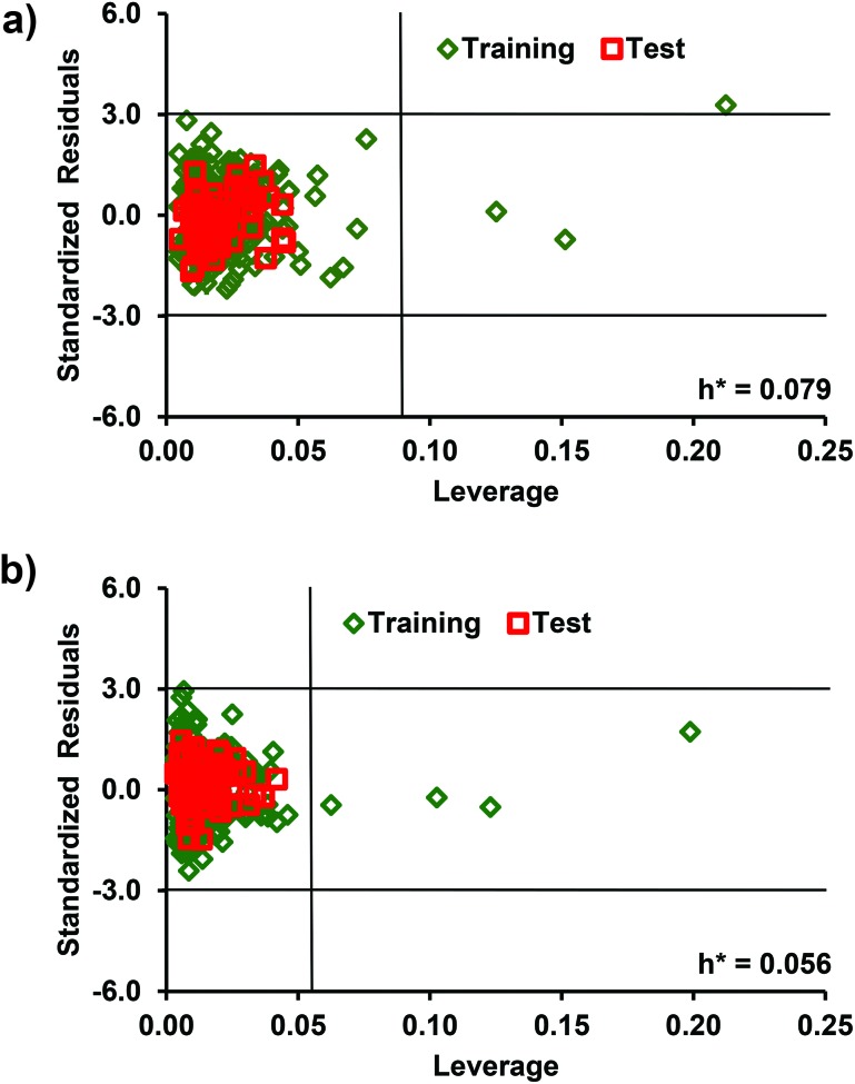
The AD of the developed QSAR models were determined by the leverage and standardization approaches. For the identification of the structurally influential and response outliers, we have developed the Williams plots (Fig. 5) using a standardized residual cut-off value of 3 against the leverage value, which showed 3 training set compounds (Abamectin, kasugamycin, spinetoram) by DTF and 4 compounds (Abamectin, kasugamycin, spinetoram, temephos) by DTB as structurally influential (Table S2, ESI†). These compounds have leverage values above the respective critical values of 0.079 (DTF) and 0.056 (DTB). However, a single compound (Abamectin) in DTF was detected as the response outlier. Further, the outliers in the training and test data were also identified using the standardization approach.49 The analysis revealed that in DTF and DTB models, 11 and 7 compounds in the training and 2 common compounds in the test were found outside the respective AD (Table S3, ESI†). The anomalous behavior of the compounds outside the AD of the models may be due to some relevant structural features present in these molecules and could not be captured by the selected descriptors. The developed QSAR models can be used to predict the endpoint toxicity of new compounds if they are located in the AD of the respective models.

Fig. 5. Williams plot for (a) the DTF-QSAR and (b) DTB-QSAR models.

The most important features of our models are the simplicity, reproducibility and interpretability of the descriptors employed for the QSAR analysis. Furthermore, our models comply with the OECD norms and implicate reliability while assessing new or existing compounds and also support the REACH policies.62 In the present study, the good performance of both QSAR models based on DTF and DTB methods may be attributed to the implementation of the bagging and boosting algorithms.

4. Conclusions

Robust and reliable EML based QSAR models have been established for predicting the multi-generation reproductive toxicity potential of the chemicals in accordance with the OECD guidelines. Accordingly, the multi-generation rat reproductive toxicity (LOAEL) data composed of 334 structurally diverse chemicals were considered for model development and validation. Relevant and interpretable structural features derived from the chemical structure were identified for model development. The generalization and external prediction abilities of the constructed models were verified using the most recent statistical test parameters, which rendered a high confidence in the developed QSARs. The excellent predictivity and generalization achieved for the models here may be attributed to the bagging and boosting algorithms implemented in the EML approaches (DTF and DTB) used for QSAR modeling. The results of the AD analysis using the leverage method revealed a single compound in DTF as the response outlier and thus confirmed the applicability of the constructed QSAR models over a wide chemical space. This study has provided a powerful tool for the prediction of the multi-generation reproductive toxicity potential of chemicals in rats, which is useful for achieving cost and effort reduction in the reproductive toxicity evaluation of new chemicals.

References

- Jensen G. E., Niemela J. R., Wedebye E. B., Nikolov N. G. SAR QSAR Environ. Res. 2008;19:631–641. doi: 10.1080/10629360802550473. [DOI] [PMC free article] [PubMed] [Google Scholar]
- National Toxicology Programme, Prenatal Developmental Toxicity Study, available at: https://ntp.niehs.nih.gov/testing/types/dev/.
- U.S. Environmental Protection Agency (U.S. EPA), Health Effects Test Guidelines OPPTS 870.3800 Reproduction and Fertility Effects, Office of Pesticides and Toxic Substances, Washington, DC, 1998, EPA 712-C-98-208
- OECD, Draft Guidance document on reproductive toxicity testing and assessment Environment, Health and Safety Publications, Series on Testing and Assessment, No. 43, OECD, 2004
- Martin M. T., Knudsen T. B., Reif D. M., Houck K. A., Judson R. S., Kavlock R. J., Dix D. J. Biol. Reprod. 2011;85:327–339. doi: 10.1095/biolreprod.111.090977. [DOI] [PubMed] [Google Scholar]
- Martin M. T., Mendez E., Corum D. G., Judson R. S., Kavlock R. J., Rotroff D. M., Dix D. J. Toxicol. Sci. 2009;110:181–190. doi: 10.1093/toxsci/kfp080. [DOI] [PubMed] [Google Scholar]
- U.S. Environmental Protection Agency (U.S. EPA). OPP Guideline 83–84: Reproductive and Fertility Effects. Pesticide Assessment Guidelines, Subdivision F, Hazard Evaluation: Human and Domestic Animals, Office of Pesticides and Toxic Substances, Washington, DC, EPA-540/9-82-025, 1982
- U.S. Environmental Protection Agency (U.S. EPA) Fed. Regist. 1996;61:56274–56322. [PubMed] [Google Scholar]
- Animal Toxicity Studies: Effects and Endpoints (Toxicity Reference Database – ToxRefDB) http://www.epa.gov/chemical-research/toxicity-forecaster-toxcasttm-data.
- Worth A. P., Bassan A., DeBruijn J., Gallegos-Saliner A., Netzeva G., Patlewicz G., Pavan M., Tsakovska I., Eisenreich S. SAR QSAR Environ. Res. 2007;18:111–125. doi: 10.1080/10629360601054255. [DOI] [PubMed] [Google Scholar]
- European Commission, Directive 2006/121/EC of the European Parliament and of the Council of 18 December 2006 amending Council Directive 67/548/EEC on the approximation of laws, regulations and administrative provisions relating to the classification, packaging and labelling of dangerous substances in order to adapt it to Regulation (EC) No. 1907/2006 concerning the Registration, Evaluation, Authorisation and Restriction of Chemicals (REACH) and establishing a European Chemicals Agency. Off. J. Eur. Union (2006), L 396/850 of 30.12.2006, Office for Official Publications of the European Communities (OPOCE), Luxembourg, 2006
- Roy K., Kar S. and Das R. N., Understanding the Basics of QSAR for Applications in Pharmaceutical Sciences and Risk Assessment, Academic Press, London, UK, 2015, ISBN: 978-0-12-801505-6. [Google Scholar]
- Dearden J. C. Int. J. Quant. Struct.—Prop. Relat. 2016;1:1–44. [Google Scholar]
- Organization for Economic Cooperation and Development (OECD), Guidance Document on the Validation of (Quantitative) Structure–activity Relationships [(Q)SAR] Models, ENV/JM/MONO 2 (2007), 2007, 1–154
- Dix D. J., Houck K. A., Martin M. T., Richard A. M., Setzer R. W., Kavlock R. J. Toxicol. Sci. 2007;95:5–12. doi: 10.1093/toxsci/kfl103. [DOI] [PubMed] [Google Scholar]
- Matthews E. J., Kruhlak N. L., Benz R. D., Ivanov J., Klopman G., Contrera J. F. Regul. Toxicol. Pharmacol. 2007;47:136–155. doi: 10.1016/j.yrtph.2006.10.001. [DOI] [PubMed] [Google Scholar]
- Rorije E., Muller A., Beekhuijzen M. E., Hass U., Heinrich-Hirsch B., Paparella M., Schenk E., Ulbrich B., Hakkert B. C., Piersma A. H. Regul. Toxicol. Pharmacol. 2011;61:251–260. doi: 10.1016/j.yrtph.2011.08.005. [DOI] [PubMed] [Google Scholar]
- Dietterich T. G. Lect. Notes Comput. Sci. 2000;1857:1–15. [Google Scholar]
- Singh K. P., Gupta S., Mohan D. J. Hydrol. 2014;511:254–266. [Google Scholar]
- Mahjoobi J., Etemad-Shahidi A. Appl. Ocean Res. 2008;30:172–177. [Google Scholar]
- Basant N., Gupta S., Singh K. P. Chemosphere. 2015;139:246–255. doi: 10.1016/j.chemosphere.2015.06.063. [DOI] [PubMed] [Google Scholar]
- Basant N., Gupta S., Singh K. P. Toxicol. Res. 2016;5:340–353. doi: 10.1039/c5tx00321k. [DOI] [PMC free article] [PubMed] [Google Scholar]
- Singh K. P., Gupta S., Kumar A., Mohan D. Chem. Res. Toxicol. 2014;27:741–753. doi: 10.1021/tx400371w. [DOI] [PubMed] [Google Scholar]
- Singh K. P., Gupta S., Basant N. RSC Adv. 2014;4:64443–64456. [Google Scholar]
- Singh K. P., Gupta S., Basant N. Chemosphere. 2015;120:680–689. doi: 10.1016/j.chemosphere.2014.10.025. [DOI] [PubMed] [Google Scholar]
- Singh K. P., Gupta S., Basant N. Chemom. Intell. Lab. Syst. 2015;140:61–72. [Google Scholar]
- Gupta S., Basant N., Singh K. P. RSC Adv. 2015;5:71153–71163. [Google Scholar]
- Gupta S., Basant N., Singh K. P. SAR QSAR Environ. Res. 2015;26:479–498. doi: 10.1080/1062936X.2015.1051584. [DOI] [PubMed] [Google Scholar]
- Zhang C., Cheng F., Sun L., Zhuang S., Li W., Liu G., Lee P. W., Tang Y. Chemosphere. 2015;122:280–287. doi: 10.1016/j.chemosphere.2014.12.001. [DOI] [PubMed] [Google Scholar]
- Cao D. S., Xu Q. S., Hu Q. N., Liang Y. Z. Bioinformatics. 2013;29:1092–1094. doi: 10.1093/bioinformatics/btt105. [DOI] [PubMed] [Google Scholar]
- ChemSpider, http://www.chemspider.com.
- Pubchem, http://pubchem.ncbi.nlm.nih.gov/compound/.
- Reitermanov Z., Data splitting, WDS'10 Proceedings of Contributed Papers, Part I, 2010, pp. 31–36..
- Singh K. P., Malik A., Singh V. K., Mohan D., Sinha S. Anal. Chim. Acta. 2005;550:82–91. [Google Scholar]
- Zhao C. Y., Zhang H. X., Zhang X. Y., Liu M. C., Hu Z. D., Fan B. T. Toxicology. 2006;217:105–119. doi: 10.1016/j.tox.2005.08.019. [DOI] [PubMed] [Google Scholar]
- Patlewicz G., Jeliazkova N., Gallegos Saliner A., Worth A. P. SAR QSAR Environ. Res. 2008;19:397–412. doi: 10.1080/10629360802083848. [DOI] [PubMed] [Google Scholar]
- Ishwaran H., Kogalur U. B. Stat. Probab. Lett. 2010;80:1056–1064. doi: 10.1016/j.spl.2010.02.020. [DOI] [PMC free article] [PubMed] [Google Scholar]
- Breiman L. Mach. Learn. 1996;24:123–140. [Google Scholar]
- Friedman J. H. Comput. Stat. Data Anal. 2002;38:367–378. [Google Scholar]
- Erdal H. I., Karakurt O. J. Hydrol. 2013;477:119–128. [Google Scholar]
- Burez J., Van den Poel D. Expert Syst. Appl. 2009;36:4626–4636. [Google Scholar]
- Karul C., Soyupak S., Cilesiz A. F., Akbay N., German E. Ecol. Model. 2000;134:145–152. [Google Scholar]
- Alexander D. L., Tropsha A., Winkler D. A. J. Chem. Inf. Model. 2015;55:1316–1322. doi: 10.1021/acs.jcim.5b00206. [DOI] [PMC free article] [PubMed] [Google Scholar]
- Roy K., Das R. N., Ambure P., Aher R. B. Chemom. Intell. Lab. Syst. 2016;152:18–33. [Google Scholar]
- Chai T., Draxler R. R. Geosci. Model. Dev. 2014;7:1247–1250. [Google Scholar]
- Rücker C., Rücker G., Meringer M. J. Chem. Inf. Comput. Sci. 2007;47:2345–2357. doi: 10.1021/ci700157b. [DOI] [PubMed] [Google Scholar]
- Mitra I., Saha A., Roy K. Mol. Simul. 2010;36:1067–1079. [Google Scholar]
- Gramatica P. QSAR Comb. Sci. 2007;26:694–701. [Google Scholar]
- Roy K., Kar S., Ambure P. Chemom. Intell. Lab. Syst. 2015;145:22–29. [Google Scholar]
- Netzeva T. I., Worth A. P., Aldenberg A. ATLA, Altern. Lab. Anim. 2005;33:155–173. doi: 10.1177/026119290503300209. [DOI] [PubMed] [Google Scholar]
- Gadaleta D., Mangiatordi G. F., Catto M., Carotti A., Nicolotti G. Int. J. Quant. Struct.—Prop. Relat. 2016;1:45–63. [Google Scholar]
- Puzyn T., Rasulev B., Gajewicz A., Hu X., Dasari T. P., Michalkova A., Hwang H. M., Toropov A., Leszczynska D., Leszczynska J. Nat. Nanotechnol. 2011;6:175–178. doi: 10.1038/nnano.2011.10. [DOI] [PubMed] [Google Scholar]
- Topliss J. G. J. Med. Chem. 1972;15:1006–1011. doi: 10.1021/jm00280a002. [DOI] [PubMed] [Google Scholar]
- Cherkasov A., Muratov E. N., Fourches D. J. Med. Chem. 2014;57:4977–5010. doi: 10.1021/jm4004285. [DOI] [PMC free article] [PubMed] [Google Scholar]
- Friedman J. H., Meulman J. J. Stat. Med. 2003;22:1365–1381. doi: 10.1002/sim.1501. [DOI] [PubMed] [Google Scholar]
- Friedman J. H. Ann. Stat. 2001;29:1189–1232. [Google Scholar]
- Hou T., Wang J., Zhang W., Wang W., Xu X. Curr. Med. Chem. 2006;13:2653–2667. doi: 10.2174/092986706778201558. [DOI] [PubMed] [Google Scholar]
- Samat N. H. A., Abdualkader A. M., Mohamed F., Abdullahie A. D. Int. J. Pharm. Pharm. Sci. 2014;6:284–290. [Google Scholar]
- Ertl P., Rohde B., Selzer P. J. Med. Chem. 2000;43:3714–3717. doi: 10.1021/jm000942e. [DOI] [PubMed] [Google Scholar]
- Afantitis A., Melagraki G., Koutentis P. A., Sarimveis H., Kollias G. Eur. J. Med. Chem. 2011;46:497–508. doi: 10.1016/j.ejmech.2010.11.029. [DOI] [PubMed] [Google Scholar]
- Tropsha A., Golbraikh A., Cho W. J. Bull. Korean Chem. Soc. 2011;32:2397–2404. [Google Scholar]
- Williams E. S., Panko J., Paustenbach D. J. CRC Crit. Rev. Toxicol. 2009;39:553–675. doi: 10.1080/10408440903036056. [DOI] [PubMed] [Google Scholar]
Associated Data
This section collects any data citations, data availability statements, or supplementary materials included in this article.