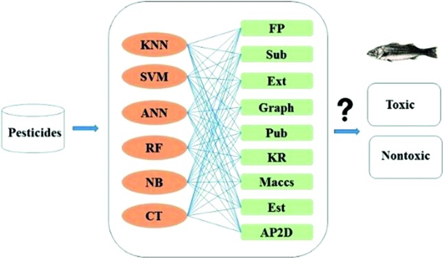
 Herein, six machine learning methods combined with nine fingerprints were used to predict aquatic toxicity of pesticides.
Abstract
Aquatic toxicity is an important issue in pesticide development. In this study, using nine molecular fingerprints to describe pesticides, binary and ternary classification models were constructed to predict aquatic toxicity of pesticides via six machine learning methods: Naïve Bayes (NB), Artificial Neural Network (ANN), k-Nearest Neighbor (kNN), Classification Tree (CT), Random Forest (RF) and Support Vector Machine (SVM). For the binary models, local models were obtained with 829 pesticides on rainbow trout (RT) and 151 pesticides on lepomis (LP), and global models were constructed on the basis of 1258 diverse pesticides on RT and LP and 278 on other fish species. After analyzing the local binary models, we found that fish species caused influence in terms of accuracy. Considering the data size and predictive range, the 1258 pesticides were also used to build global ternary models. The best local binary models were Maccs_ANN for RT and Maccs_SVM for LP, which exhibited accuracies of 0.90 and 0.90, respectively. For global binary models, the best model was Graph_SVM with an accuracy of 0.89. Accuracy of the best global ternary model Graph_SVM was 0.81, which was a little lower than that of the best global binary model. In addition, several substructural alerts were identified including nitrobenzene, chloroalkene and nitrile, which could significantly correlate with pesticide aquatic toxicity. This study provides a useful tool for an early evaluation of pesticide aquatic toxicity in environmental risk assessment.
1. Introduction
Pesticides have become essential products in our daily life. Modern pesticides are usually used to protect plants and crops, but the release of pesticides continues to affect all aspects of natural resources including the atmosphere, water, soil and wildlife. Therefore, it is of importance to assess the potential risk of pesticides to our health and the environment. For water pollution, fishes are usually used as the model species to evaluate aquatic toxicity; especially, under the EC Regulation 1107/2009 (European Pesticide Regulation No. 1107/2009), there is a requirement for registrants to assess whether pesticide metabolites are potentially harmful to the environment and fish acute toxicity assessments may be carried out. The experimental determination of acute fish toxicity usually involves an animal test, resulting in LC50 (lethal concentration 50%) values. However, there is an increasing need to reduce or replace animal tests for regulatory purposes. Both in vitro and in silico approaches are hence developed as non-animal alternatives.1–5
In practice, knowing whether a compound is toxic or non-toxic, highly toxic or slightly toxic, rather than its exact toxicity value is the first step of hazard risk assessment. The United States Environmental Protection Agency (U.S. EPA) has defined chemical toxicity categories of aquatic organisms, as shown in Table 1, which are suitable for the abovementioned purpose. According to these categories, chemical aquatic toxicity can be divided into five categories: very highly toxic, highly toxic, moderately toxic, slightly toxic, and practically nontoxic.
Table 1. Chemical toxicity categories in aquatic organisms.
| Toxicity category | Aquatic organism acute concentration (PPM) | Binary classification | Ternary classification |
| Very highly toxic | <0.1 | 1 | 2 |
| Highly toxic | 0.1–1 | 1 | 2 |
| Moderately toxic | 1–10 | 1 | 1 |
| Slightly toxic | 10–100 | 0 | 0 |
| Nontoxic | >100 | 0 | 0 |
A large number of computational methods have been used for the development of reliable prediction models of pesticide toxicity on fishes. These models can be divided into local models and global models.6–9 Local models are based on the mode of action (MOA)10–13 and specific functional groups.14–18 However, the application of such models is limited due to the pre-requirement of information on the MOA and functional groups in the chemicals. Recently, local models based on toxicity data in a single test species and global models based on combined toxicity data for different test species have been proposed.19–21 Global models have the advantage that they are applicable for many compounds across mechanisms of action and structure.22,23 To date, local models24–26 have some limitations in their application, while global models19,27,28 have a larger applicability domain but limited numbers of pesticides. Compared with the local ones, global models usually apply different toxicity data in model building, and hence, they are more difficult to be developed with high accuracy than local ones to some extent.
However, most of these models are built by statistic methods with limited compounds and molecular descriptors.19 In recent years, several approaches to machine learning have emerged as unbiased methods for building predictive models.29–31 For example, Nikita used decision tree forest and decision tree boost approaches with descriptors to build models for predicting toxicity data of 318 pesticides in O. mykiss (96 h LC50) and 294 pesticides in L. macrochirus (96 h LC50).28 Hence, in this study, we aim to use machine learning methods to build both local and global models to predict pesticide aquatic toxicity in various fish species. High-quality diverse data were first collected from databases. Then, nine fingerprints were used to represent the chemicals, and six machine learning methods were applied to build binary and ternary classification models for the prediction of toxicity. Two fish species, i.e. rainbow trout (RT, O. mykiss) and bluegill sunfish (LP, L. macrochirus), were used to build local models, and only one fish species was used in each local model. In the global models, the two fish species used above and some other fishes were used together. We also compared our models with ECOSAR,32 a computerized predictive system for estimating aquatic toxicity, in terms of accuracy. At last, substructural alerts33 of pesticides were analyzed by information gain and substructure frequency analysis methods. The predictive models built here would be very helpful for the assessment of chemical aquatic toxicity.
2. Materials and methods
2.1. Data collection and preparation
Acute aquatic toxicity data of all pesticides were obtained from the Pesticide Properties Database (PPDB 2015), which has evolved from a database that originally accompanied the EMA (Environmental Management for Agriculture) software and has been systematically developed further and expanded with funding from other research projects and earned income. Only the data obtained in 96 hours for fresh water fish with LC50 values were chosen for this study. 2D chemical structures were obtained from Aggregated Computational Toxicology Resource (ACToR) database of the U.S. EPA by CAS Registry Number (CASRN) using in-house scripts. All the structures were double checked with the PubChem database.34 The data were prepared by the following steps. First, the compounds including inorganic compounds, organometallic compounds, salts and mixtures were removed. Next, based on U.S. EPA guidelines of toxicity categories (Table 1), the compounds were classified into five levels. It is easy to clear the original data from PPDB, as each compound has only one toxic value. Finally, the dataset was randomly divided into two sets for model building and external validation in the ratio of 8 : 2.
2.2. Molecular description
Molecular fingerprints are widely used in molecular description, similarity searching and classification. Nine fingerprints were used in this work. They are Fingerprint (FP), Extended fingerprint (Ext), Estate fingerprint (Est), MACCS fingerprint (Maccs), PubChem fingerprint (Pub), Substructure fingerprint (Sub) Graphonly fingerprint (Graph), AP2D fingerprint (AP2D) and Klekota-Roth fingerprint (KR). All the fingerprints were calculated using PaDEL-Descriptor software.35
2.3. Model building
Both local and global models were constructed, and binary and ternary classification models were built separately. In the binary classification models, very highly toxic, highly toxic and moderately toxic data were combined as one class, and the remaining slightly toxic and nontoxic data were combined as the other class. While in the ternary classification models, very highly toxic and highly toxic data were combined as one class; moderately and slightly toxic data were used as the second class, and nontoxic data were used as the third class. Six machine learning methods (Naïve Bayes (NB), Artificial Neural Network (ANN), k-Nearest Neighbor (kNN), Classification Tree (CT), Random Forest (RF) and Support Vector Machine (SVM)) were employed for model building. The first five methods were performed on Orange Canvas 2.7 (available free of charge at the website: http://www.ailab.si/orange/). The SVM algorithm was performed on the LIBSVM 3.16 package.36
NB is a simple classification method based on the Bayes theorem for conditional probability.37 Neural networks are good at fitting non-linear functions and recognizing patterns;38 it was trained for classification by using the representative fingerprint of each class. The kNN classification method is based on the closest training examples in a feature space;39 it was built by Orange and the parameter of k was set to ten in the present work. Classification tree analysis is one of the main techniques used in data mining.40,41 in this study, orange with the default setting was used to perform the classification models by these four methods. Random forest is also an ensemble learning method for classification (and regression) that operates by constructing a multitude of decision trees at training time and outputting the class that is the mode of the classes outputted by individual trees.42 In this study, the number of trees in the forest was set as 10, stop splitting nodes as 5, and the other parameters were the default values. SVM is an excellent kernel-based tool for binary data classification and can be used for classification and regression analysis,43 and it has been successfully employed to solve many binary classification problems by our group44,45 and many others.46,47 In this study, the Gaussian radial basis function (RBF) kernel was used. RBF is a popular kernel function used in SVM classification; the parameters C and γ for RBF kernel were tuned on the training set by a 10-fold cross-validation.
2.4. Evaluation of model performance
Ten-fold cross-validation31 was used to evaluate the robustness of the models, while external validation set48 was used to assess the predictive accuracy of the models. All models were evaluated by the counts of true positives (TP), true negatives (TN), false positives (FP), and false negatives (FN). The sensitivity (SE), specificity (SP) and classification accuracy (CA) were also calculated. In binary classification, the sensitivity, specificity, and overall predictive accuracy (CA) of the models were calculated as follows:
 |
1 |
 |
2 |
 |
3 |
In ternary classification models, the overall predictive accuracy was calculated as follows:
 |
4 |
Here, N0–0 means high toxicity was predicted as high toxicity; N1–1 means moderate toxicity was predicted as moderate toxicity; N2–2 means non-toxicity was predicted as non-toxicity; and NTotal represents the total number in the data set.
2.5. Analysis of substructural alerts
The privileged substructures or substructural alerts are defined as molecular functional groups that are known to induce toxicity. Their appearance in a chemical structure alerts the researchers to potential toxicities of the test compounds.33 Hence, they are important tools to predict toxicity. We used the method of information gain (IG) to search substructural fragments, and the detailed method has been described in our previous papers.45,49,50 Another method, named ChemoTyper, was also used to identify toxic substructures.51
3. Results
3.1. Data collection and analysis
Acute aquatic toxicity data of all pesticides were obtained from the Pesticide Properties Database (PPDB 2015). After standardization of the data, we collected acute aquatic toxicity data of 1258 diverse pesticides including 828 on RT, 151 on LP and 278 on other fish species. All these data were separated into training sets and external validation sets randomly in the ratio of 8 : 2. The SMILES strings and toxic classes of all the data sets are listed in the ESI (SI1†). The distributions of compounds in different toxic classes of training sets and external validation sets are listed in Table 2. The number of pesticides in the training set and external validation set of the local models was 663 and 166 for RT and 120 and 31 for LP. For the global models, the number of unique compounds in the training set and external validation set was 1005 and 253, respectively.
Table 2. Statistical data of pesticides in different toxic classes of training sets and external validation sets.
| Set name | Total number | Training set |
External validation set |
||||||||
| Very highly toxic | Highly toxic | Moderately toxic | Slightly toxic | Nontoxic | Very highly toxic | Highly toxic | Moderately toxic | Slightly toxic | Nontoxic | ||
| All | 1258 (1005 : 253) | 150 | 166 | 238 | 219 | 232 | 37 | 44 | 58 | 55 | 59 |
| RT | 829 (663 : 166) | 104 | 116 | 154 | 139 | 150 | 25 | 30 | 39 | 35 | 37 |
| LP | 151 (120 : 31) | 24 | 24 | 25 | 27 | 20 | 6 | 7 | 6 | 6 | 6 |
| Others | 278 (222 : 56) | 22 | 26 | 61 | 53 | 60 | 6 | 7 | 13 | 14 | 16 |
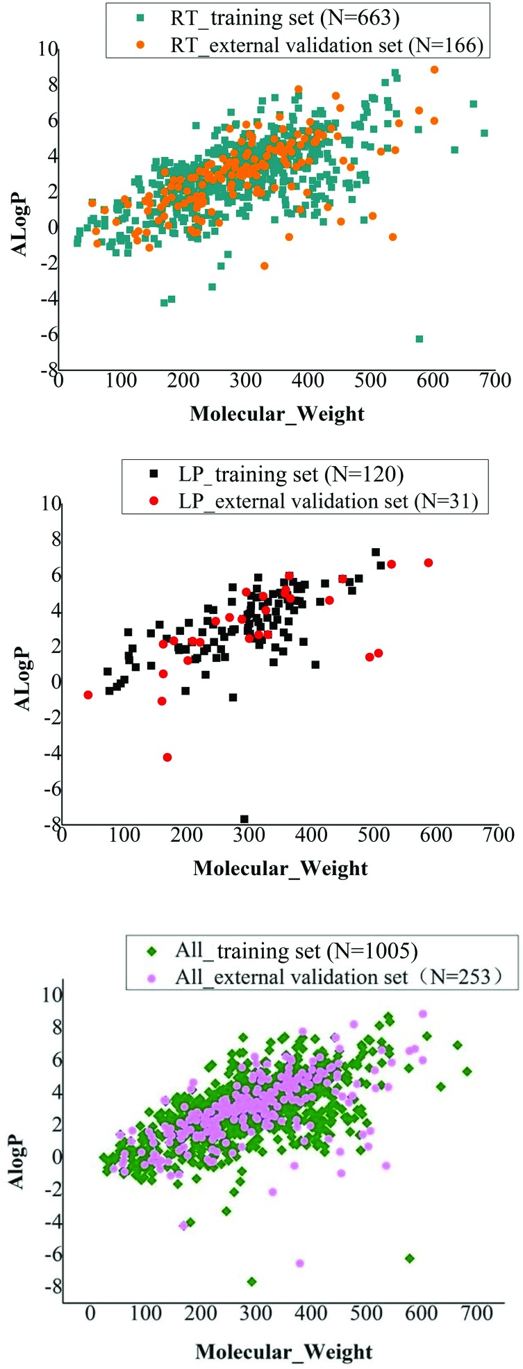
Chemical diversity is important for building a global and robust classification model. Therefore, we used chemical space and Tanimoto similarity to investigate the chemical diversity. In this study, the chemical space distributed by these data sets was defined by the molecular weight (MW) and A log P. The chemical space distribution plot of the RT training set and external validation set is depicted in Fig. 1A and that of LP training set and external validation set is depicted in Fig. 1B; chemical space distribution plot for all fish training and external validation sets are depicted in Fig. 1C. From the chemical space analysis, we found that data in the training and external validation sets were distributed in the same chemical space, which indicated that these models had a reasonable applicability domain.
Fig. 1. Chemical space distribution of the training and external validation sets of RT, LP and all fish sets. N represents the number of chemicals in different datasets. Chemical space was defined by molecular weight (MW) and Ghose-Crippen LogKow (A log P).
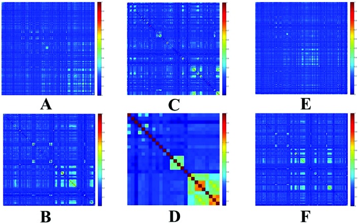
Tanimoto coefficient was used to evaluate the diversity of chemicals. The heat maps of Tanimoto similarity index of the above three datasets and their external validation sets are shown in Fig. 2. The color closer to red in the heat map (with high Tanimoto similarity index) means that the compounds are more similar; on the contrary, the color closer to dark blue (with low Tanimoto similarity index) means that the compounds have higher diversity. The average Tanimoto similarity indexes were 0.17 for RT training set, 0.16 for RT external validation set, 0.17 for LP training set and 0.25 for LP external validation set. Tanimoto similarity indexes for all fish training set and the external validation set were 0.16 and 0.16, respectively. These results indicated these datasets were chemically diverse.
Fig. 2. Tanimoto similarity index for each training set and external validation set. A: RT training set; B: RT external validation set; C: LP training set; D: LP external validation set; E: all fish training set; F: all fish external validation set.
3.2. Performance of binary classification models
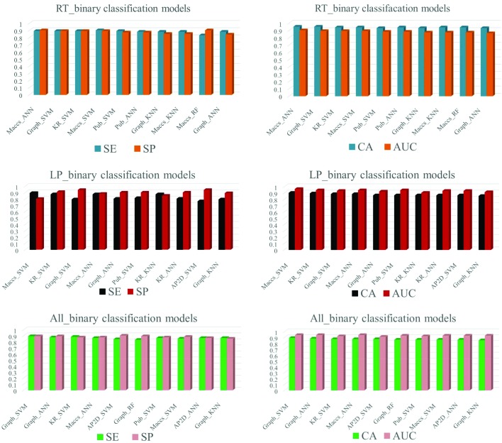
In this study, the local and global binary classification models were built using nine fingerprints combined with six machine learning methods, including NB, ANN, kNN, CT, RF and SVM. The models were validated by ten-fold cross-validation and external set validation. The CA, SE, SP and AUC values of top 10 classification models for ten-fold cross-validation are summarized in Fig. 3, and detailed values of all binary classification models are listed in ESI (SI2†).
Fig. 3. Top 10 binary models of RT, LP and all fish training set. AP2D: AP2D fingerprint, Est: estate fingerprint, Ext: extended fingerprint, FP: fingerprint, Graph: graphonly fingerprint, KR: Klekota-Roth fingerprint, Maccs: MACCS fingerprint, Pub: PubChem fingerprint, Sub: substructure fingerprint; ANN: artificial neural network, CT: classification tree, kNN: k-nearest neighbor, NB: naïve bayes, RF: random forest, SVM: support vector machine.
Ten-fold cross-validation of the training set was performed to evaluate models’ robustness. The best models were selected based on the values of CA and AUC. For local models, the best model of RT was Maccs_ANN (CA = 0.90, SP = 0.90, SE = 0.90, AUC = 0.95), the best model of LP was Maccs_SVM (CA = 0.90, SP = 0.89, SE = 0.90, AUC = 0.96). For global models, the best model was Graph_SVM (CA = 0.89, SP = 0.89, SE = 0.89, AUC = 0.94).
The values of CA and AUC of all local and global models were greater than 0.6, and for both local and global models, the values of SE and SP were greater than 0.7, except some models built with NB (SI2†). For RT and LP local models, comparing the performance of the six machine learning methods when using the same fingerprint, SVM and ANN performed better than the others and NB performed the worst. Comparing the performance of nine fingerprints when using the same algorithm, Maccs yielded the best results and KR and Graph also performed pretty well. For global models, we found the method with the worst performance was NB, but the best fingerprint was Graph.
3.3. Performance of ternary classification models
In this study, 65% of the total data was about RT; considering the data size, only global ternary classification models were built using nine fingerprints combined with six machine learning methods, including NB, ANN, KNN, CT, RF and SVM. All the models were validated by ten-fold cross-validation and external set validation. The CA, SE and AUC values of the top 10 models for ten-fold cross-validation are summarized in Table 3 and the detailed values of all ternary classification models are listed in ESI 2 (SI2†). The best model Graph_SVM (CA = 0.81, SE_0 = 0.67, SE_1 = 0.89, SE_2 = 0.80, AUC = 0.92) was selected based on the values of CA and AUC.
Table 3. Performance of top 10 ternary classification models of all fish species for the ten-fold cross validation.
| Model a | AUC | CA | SE_0 b | SE_1 b | SE_2 b |
| Graph_SVM | 0.92 | 0.81 | 0.67 | 0.89 | 0.80 |
| AP2D_KNN | 0.90 | 0.80 | 0.72 | 0.81 | 0.84 |
| AP2D_SVM | 0.93 | 0.80 | 0.65 | 0.88 | 0.81 |
| Graph_ANN | 0.91 | 0.79 | 0.71 | 0.81 | 0.82 |
| Maccs_SVM | 0.91 | 0.79 | 0.65 | 0.85 | 0.82 |
| AP2D_ANN | 0.90 | 0.79 | 0.67 | 0.83 | 0.83 |
| Graph_KNN | 0.90 | 0.77 | 0.67 | 0.79 | 0.81 |
| Pub_SVM | 0.92 | 0.77 | 0.65 | 0.84 | 0.77 |
| KR_SVM | 0.91 | 0.77 | 0.66 | 0.83 | 0.76 |
| Maccs_ANN | 0.90 | 0.76 | 0.68 | 0.79 | 0.80 |
aAP2D: AP2D fingerprint, Est: estate fingerprint, Ext: extended fingerprint, FP: fingerprint, Graph: graphonly fingerprint, KR: Klekota-Roth fingerprint, Maccs: MACCS fingerprint, Pub: PubChem fingerprint, Sub: substructure fingerprint; ANN: artificial neural network, CT: classification tree, kNN: k-nearest neighbor, NB: naïve bayes, RF: random forest, SVM: support vector machine.
bSE_0: SE value of data labeled class 0, SE_1: SE value of data labeled class 1, SE_2: SE value of data labeled class 2.
Compared with the results of binary classification for global models, all ternary classification models performed much worse. The values of CA and AUC of these ternary models were much lower, and the values of SE for each class were much lower too. By comparing the performance of the six machine learning methods when using the same fingerprint, we found that SVM and ANN performed better than the others and NB performed the worst, which is the same as that for the binary classification models. Comparing the performance of the nine fingerprints, when using the same algorithm, fingerprints Graph and AP2D yielded better results than other seven fingerprints.
3.4. External set validation
3.4.1. External set validation of local binary classification models
To further study the predictive ability of these classification models, all local models were evaluated by external set validation. The detailed results are shown in SI2.† For RT, the top 5 prediction results are listed in Table 4; Maccs_ANN performed the best and machine learning method SVM performed pretty well. For LP, performance of top 5 binary classification models for the external validation set is listed in Table 5; Est_CT gave the best performance, which seems very strange. We think that the number of external test sets caused this difference, as only 31 pesticides were used as external test sets for LP fish.
Table 4. Performance of top 5 binary classification models of RT for the external validation set.
| Model a | AUC | CA | SP | SE |
| Maccs_ANN | 0.88 | 0.81 | 0.81 | 0.82 |
| Maccs_SVM | 0.89 | 0.81 | 0.78 | 0.84 |
| KR_SVM | 0.87 | 0.81 | 0.77 | 0.84 |
| Est_SVM | 0.89 | 0.81 | 0.82 | 0.79 |
| Ext_SVM | 0.83 | 0.80 | 0.85 | 0.75 |
aAP2D: AP2D fingerprint, Est: estate fingerprint, Ext: extended fingerprint, FP: fingerprint, Graph: graphonly fingerprint, KR: Klekota-Roth fingerprint, Maccs: MACCS fingerprint, Pub: PubChem fingerprint, Sub: substructure fingerprint; ANN: artificial neural network, CT: classification tree, kNN: k-nearest neighbor, NB: naïve bayes, RF: random forest, SVM: support vector machine.
Table 5. Performance of top 5 binary classification models of LP for the external validation set.
| Model a | AUC | CA | SP | SE |
| Est_CT | 0.82 | 0.81 | 0.89 | 0.74 |
| AP2D_KNN | 0.76 | 0.79 | 0.89 | 0.71 |
| KR_CT | 0.77 | 0.76 | 0.89 | 0.65 |
| AP2D_RF | 0.74 | 0.76 | 0.78 | 0.74 |
| Graph_NB | 0.76 | 0.74 | 0.82 | 0.68 |
aAP2D: AP2D fingerprint, Est: estate fingerprint, Ext: extended fingerprint, FP: fingerprint, Graph: graphonly fingerprint, KR: Klekota-Roth fingerprint, Maccs: MACCS fingerprint, Pub: PubChem fingerprint, Sub: substructure fingerprint; ANN: artificial neural network, CT: classification tree, kNN: k-nearest neighbor, NB: naïve bayes, RF: random forest, SVM: support vector machine.
3.4.2. External set validation of global binary classification models
The external validation sets were used to evaluate predictive ability of all models in ten-fold cross-validation. The detailed results of the external set validation are listed in Table 6. The best model for the global binary model was Maccs combined with ANN algorithm (CA = 0.83, SP = 0.83, SE = 0.82, AUC = 0.89), which performed fourth best in the ten-fold cross-validation, while the best model in the ten-fold cross-validation did not perform very well in the external set validation. The ranking by CA values of these external validation results were different from that in the ten-fold cross-validation. But in the external set validation, we found that ANN and SVM performed better than other algorithms and Maccs performed better than other fingerprints, which is in accordance with the results of ten-fold cross-validation.
Table 6. Performance of top 5 binary classification models of all fish for the external validation set.
| Model a | AUC | CA | SP | SE |
| Maccs_ANN | 0.89 | 0.83 | 0.83 | 0.82 |
| Est_SVM | 0.88 | 0.82 | 0.86 | 0.80 |
| Maccs_SVM | 0.85 | 0.82 | 0.89 | 0.78 |
| KR_SVM | 0.85 | 0.80 | 0.86 | 0.77 |
| Pub_SVM | 0.83 | 0.81 | 0.87 | 0.76 |
aAP2D: AP2D fingerprint, Est: estate fingerprint, Ext: extended fingerprint, FP: fingerprint, Graph: graphonly fingerprint, KR: Klekota-Roth fingerprint, Maccs: MACCS fingerprint, Pub: PubChem fingerprint, Sub: substructure fingerprint; ANN: artificial neural network, CT: classification tree, kNN: k-nearest neighbor, NB: naïve bayes, RF: random forest, SVM: support vector machine.
3.4.3. External set validation of ternary classification models
Although the results of all global ternary classification models were not as good as binary classification models, the external validation sets were also used to evaluate the predictive ability of all models. The detailed results of the top 5 external set validation sets are listed in Table 7. The best model for the global ternary model was Pub combined with SVM algorithm (CA = 0.67, SE_0 = 0.67, SE_1 = 0.67, SE_2 = 0.68, AUC = 0.85), which did not perform very well in the ten-fold cross-validation. The results of external set validation further explained that for the ternary global model, SVM performed better than other algorithms and Pub performed better than other fingerprints.
Table 7. Performance of top 5 ternary classification models of all fish for the external validation set.
| Model a | AUC | CA | SE_0 b | SE_1 b | SE_2 b |
| Pub_SVM | 0.85 | 0.67 | 0.67 | 0.67 | 0.68 |
| Est_SVM | 0.84 | 0.66 | 0.61 | 0.70 | 0.62 |
| KR_SVM | 0.84 | 0.65 | 0.62 | 0.70 | 0.60 |
| Pub_KNN | 0.80 | 0.65 | 0.58 | 0.66 | 0.68 |
| FP_SVM | 0.81 | 0.63 | 0.63 | 0.66 | 0.59 |
aAP2D: AP2D fingerprint, Est: estate fingerprint, Ext: extended fingerprint, FP: fingerprint, Graph: graphonly fingerprint, KR: Klekota-Roth fingerprint, Maccs: MACCS fingerprint, Pub: PubChem fingerprint, Sub: substructure fingerprint; ANN: artificial neural network, CT: classification tree, kNN: k-nearest neighbor, NB: naïve bayes, RF: random forest, SVM: support vector machine.
bSE_0: SE value of data labeled class 0, SE_1: SE value of data labeled class 1, SE_2: SE value of data labeled class 2.
3.5. Comparison with ECOSAR
The Ecological Structure Activity Relationships (ECOSAR) program is a computerized predictive system that estimates aquatic toxicity. To compare the accuracy of our models, ECOSAR was used to predict chemical aquatic toxicity of our both local and global external validation sets. For local external validation set, ECOSAR gave CA = 0.72, SP = 0.65, and SE = 0.79, and for global external validation set, ECOSAR gave CA = 0.68, SP = 0.61, and SE = 0.77. These indicated that our models had greater prediction accuracy for pesticide acute toxicity to fish.
3.6. Identification of toxic substructures
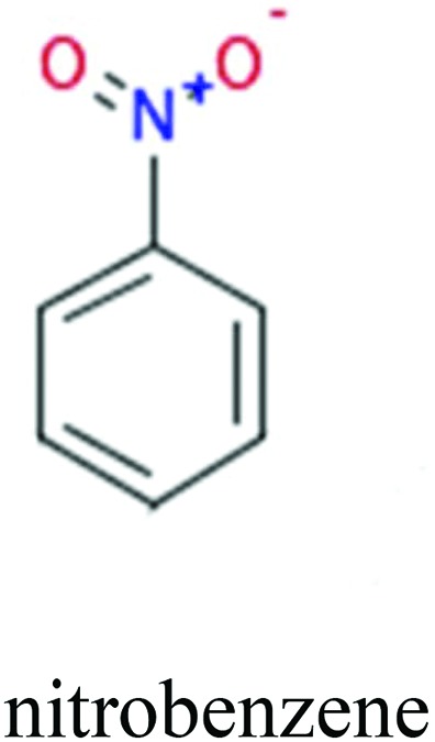
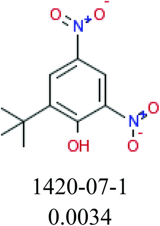
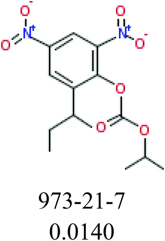
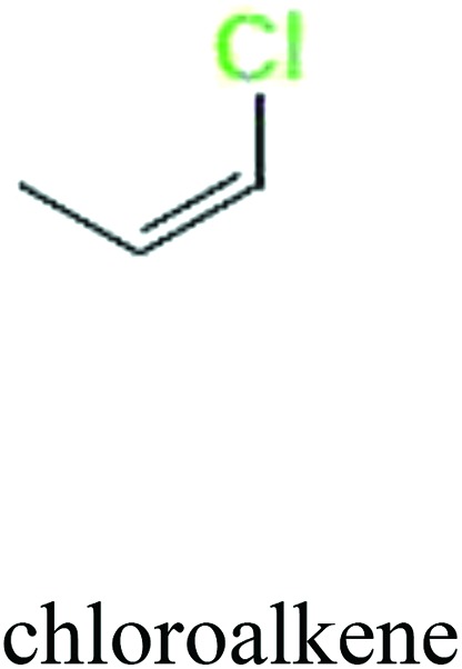
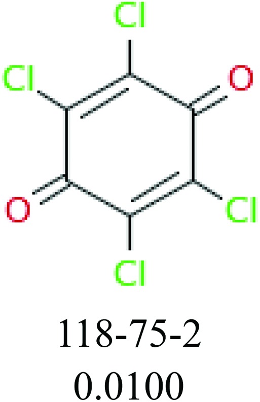
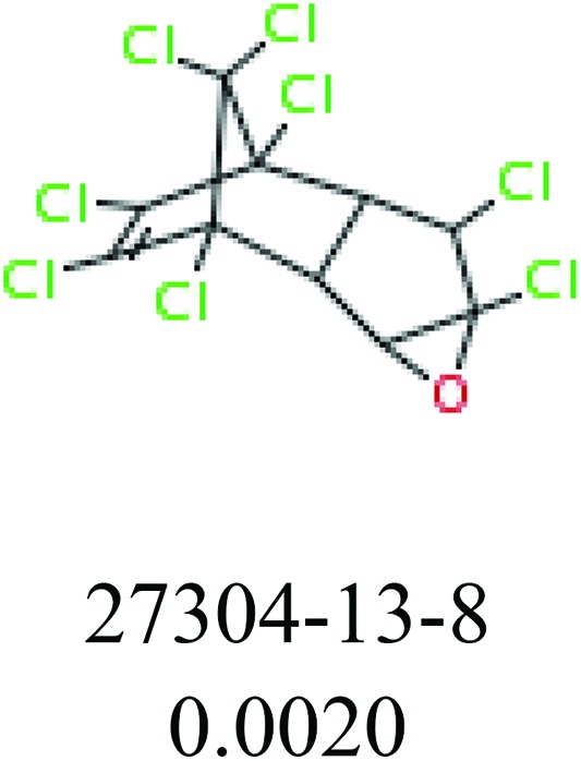
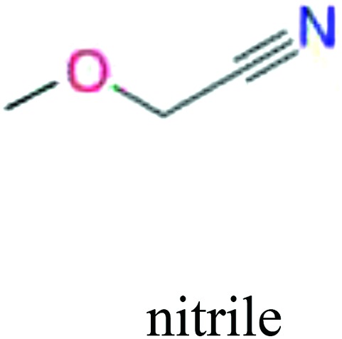
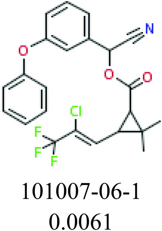
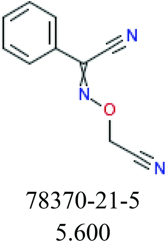
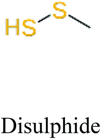
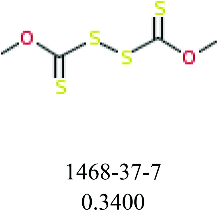
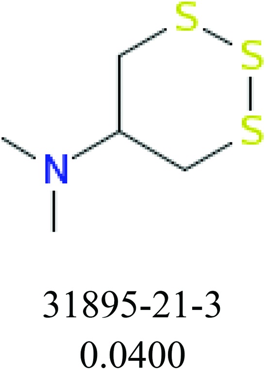
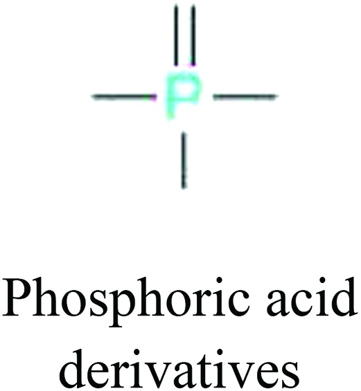
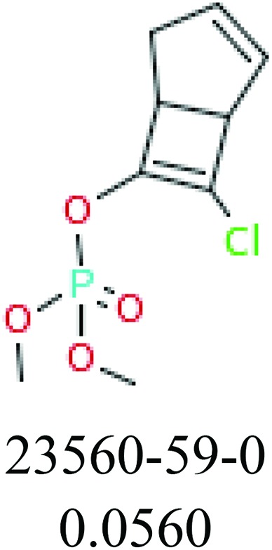
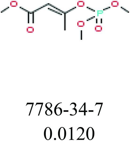
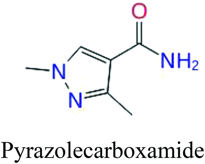
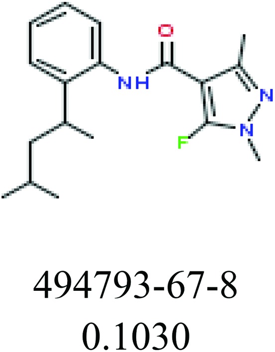
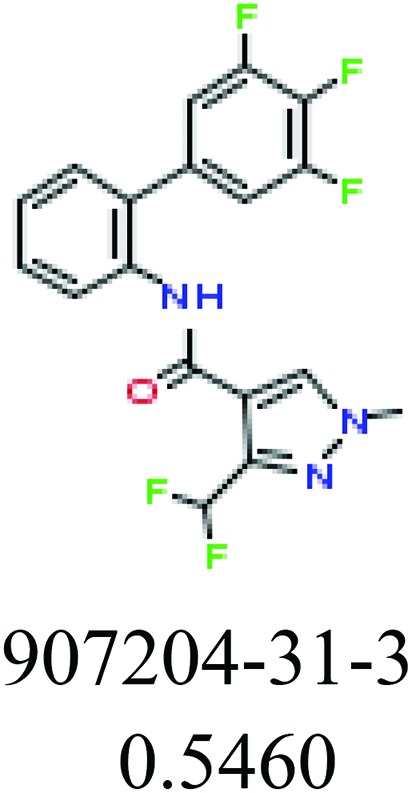
To investigate structural differences between toxic and nontoxic compounds, the IG method was performed to identify toxic substructures in all datasets based on Maccs fingerprint. According to the values of IG, p (positive) and n (negative), we obtained 26 substructures, and the top 6 substructures are shown in Table 8 for further analysis.
Table 8. Common substructural alerts identified in all fish data.
| Fragments (structure name) | Example 1 (CAS number) (IC50 value ppm) | Example 2 (CAS number) (IC50 value ppm) |
|
|
|
|
|
|
|
|
|
|
|
|
|
|
|
|
|
|
ChemoTyper was also used to validate the toxic substructures found above, and most of the six substructures such as nitrile, chloroalkene, disulphide and phosphoric acid derivatives in Table 8 can also be identified by ChemoTyper.
4. Discussion
4.1. Fish species influence predictive effect of models
As is known, data quality plays an important role in the results of classification models. In binary classification models, for example, we built local models for RT and LP and global models for all data. We found that fish species do impact predictive effect of classification models by comparing results of the local and global models. To further validate if fish species influence the accuracy of classification models, data named others was further used to build binary classification models; the toxicity values of 278 pesticides were included many fish species, such as Pimephales promelas, Brachydanio rerio, Cyprinodon, Cyprinus carpio and some other unknown species. All toxicity data which were about more than 10 varieties of fish were used to build binary classification models to prove fish species have a significant impact on the accuracy of classification models. CA and other evaluation index value results of binary classification models built in this section are shown in SI2.† Then, we found that CA values reduced by more than 6% and SE values by about 2% on separately comparing values with RT and LP binary classification models.
4.2. Comparison of different fingerprints and machine learning methods
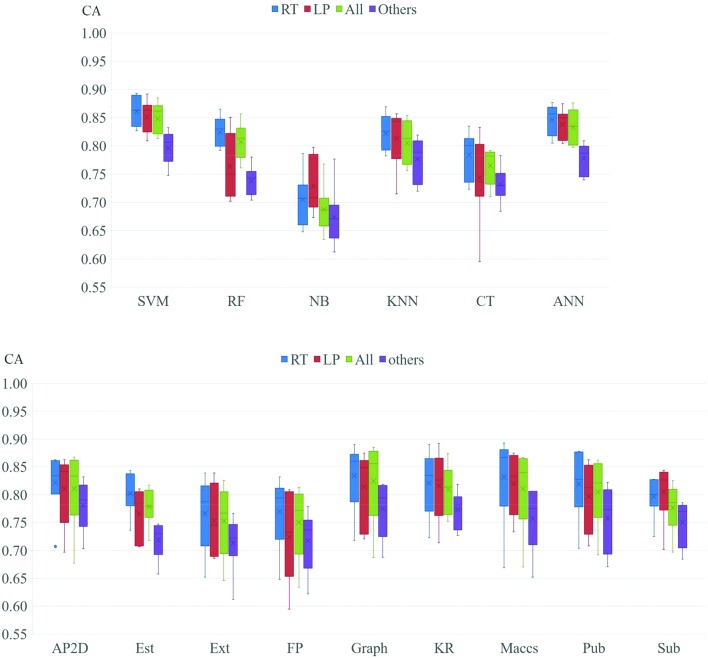
Nine fingerprints and six types of machine learning methods were used to build local and global classification models, and then we found which method and fingerprint perform the best. CA value distribution was considered as the evaluation index of each method and fingerprint. Boxplots of all methods and fingerprints that can intuitively describe the distribution of CA values are shown in Fig. 4. By comparing six different machine learning methods, we found that SVM gave the best performance for all local models and global models and ANN was the second-best method with a CA value just a little lower than that of SVM. Next in order were KNN, RF and CT. NB gave the worst performance. For both local and global models, the prediction accuracy of six methods showed a lot of consistencies. Thus, it can be concluded that the performance of each method was less affected by fish species. By comparing the nine fingerprints, we found that Graph, KR, Maccs, Pub and AP2D gave good performance in most of the models, while the other four fingerprints (Est, Ext, FP and Sub) did not perform very well. By comparing the five fingerprints with good performance, we found that Maccs did best in local models such as RT and LP, while Graph and AP2D gave high accuracy value in All fish and Others fish models. So, we speculated that fish species influence the performance of each fingerprint and Maccs is more applicable to build models for a single species, while Graph and AP2D are more suitable to build prediction models for various species of fish.
Fig. 4. Boxplots of different machine learning methods and different fingerprints. AP2D: AP2D fingerprint, Est: estate fingerprint, Ext: extended fingerprint, FP: fingerprint, Graph: graphonly fingerprint, KR: Klekota-Roth fingerprint, Maccs: MACCS fingerprint, Pub: PubChem fingerprint, Sub: substructure fingerprint; ANN: artificial neural network, CT: classification tree, kNN: k-nearest neighbor, NB: naïve bayes, RF: random forest, SVM: support vector machine.
4.3. Analysis of substructural alerts
Several common substructures in Table 5 have been reported before, such as nitrobenzene, nitrile and phosphoric acid derivatives. Toxicity of nitrobenzene derivatives in fish is determined by both hydrophobicity (expressed by octanol/water partition coefficient) and rate of reduction of the nitro group (expressed by either electrochemical halfwave reduction potential or Hammett σ values).52 For nitrile families, the acute toxicity is caused by their character of strong electron-withdrawing.53,54 Phosphoric acid esters are well-known insecticides that act specifically by inhibiting acetylcholinesterase (AChE). The enzyme AChE is inhibited by phosphorylation of a hydroxy group in serine.55 It can also affect the cholinergic receptor directly, leading the next neuron or effector to exhibit excessive excitement or inhibition.56 Other substructures such as chloroalkene and disulphide can cause infestation of nerve centers or injury of internal organs.57,58 Because of highly biologically active of pyrazolyl group and formamido group, pyrazolecarboxamide is widely used in pesticides. But fish experiments show that pyrazolecarboxamide can lead to fluctuation of both superoxide dismutase (SOD) and catalase (CAT) levels in all tissues.59 These substructural alerts are very important in ecological risk assessment and can help us evaluate whether pesticides can be freely used in water.
4.4. Comparison with others’ work
Pesticides have become essential products in everyday life, and many researchers have already paid attention to pesticide aquatic toxicity prediction. A fragment-based QSAR approach was presented to correlate 96 h LC50 acute toxicity on rainbow trout by Mose’ Casalegno.60 All 282 pesticides were used and quantitative toxicity prediction yielded results for the training set (R2TR 0.85) and test set (R2TS 0.75). Results of this single fish species seemed really good, but only 282 pesticides were considered; the lack of data might pose an insurmountable barrier in toxicity prediction for pesticides’ complex structures and tremendous amount. In another previous study,61 674 acute values linked to chemical MOA was developed for fish. These 674 molecules included four aquatic species (three fish species and one Daphnia magna): rainbow trout (Oncorhynchus mykiss), fathead minnow (Pimephales promelas), bluegill (Lepomis macrochirus), and cladoceran (Daphnia magna). In the fish species, estimated values were highly correlated with measured values (R2 > 0.87). In fact, it is always more valuable to know whether it is toxic or not than to know the specific toxicity value for pesticides. At present, there are few predictive models for the classification of pesticide toxicity. In this work, many more pesticides (1258) were studied, and it could be applied to a variety of toxicity predictions. For example, the local models can help us predict toxicity of pesticide molecules to specific species of fish such as RT or LP. When the species of fish is not considered, global models can be used.
5. Conclusions
In the present study, nine fingerprints combined with six machine learning methods were used to build both binary and ternary classification models, which were based on a data set of 1258 pesticides, aiming at predicting the acute toxicity for fish. Based on the values of CA and AUC, the best models for RT, LP and All fish groups were determined. For RT binary classification models, Maccs_ANN gave the best result (CA = 0.90, SP = 0.90, SE = 0.90, AUC = 0.95); for LP binary classification models, Maccs_SVM (CA = 0.90, SP = 0.89, SE = 0.90, AUC = 0.96) performed the best; and for global models, the best model was Graph_SVM (CA = 0.89, SP = 0.89, SE = 0.89, AUC = 0.94). From the above results, we can conclude that for binary models, SVM and ANN are two good machine learning methods for both local and global models, which means that the accuracy of each method has nothing to do with fish species. In contrast, fish species influence the performance of each fingerprint, and we can conclude that fingerprint Maccs is more applicable to local models, while fingerprint Graph is more suitable to build global models. Considering the data size, we neglected influence of different fish species and built ternary classification models for all 1258 pesticides. Graph_SVM gave the best result (CA = 0.81, SP = 0.95, SE = 0.67, AUC = 0.93), which is consistent with global binary models which show that SVM and Graph perform better than others. These results imply that our models are robust and reliable and demonstrate that it is feasible to develop classification models using fingerprints along with machine learning methods. Moreover, the substructural alerts were identified, which can be used to distinguish pesticide acute toxicity for fish by means of information gain and substructure frequency analysis. These substructural alerts appeared more frequently in pesticides with high fish toxicity, and thus, they should be responsible for acute aquatic toxicity, which would be helpful for understanding reaction mechanism. In summary, this study developed a series of predictive models including local and global and binary and ternary models; all these models can meet different prediction needs for acute aquatic toxicity of pesticides. The identified toxic substructures responsible for pesticide aquatic toxicity can be used for pesticide screening in the early stages of pesticide development.
Conflicts of interest
There are no conflicts of interest to declare.
Supplementary Material
Acknowledgments
We gratefully acknowledge the financial support from the National Natural Science Foundation of China (Grants 81273438 and 81373329).
Footnotes
†Electronic supplementary information (ESI) available: The SMILES strings and toxic classes of all chemicals are listed in SI1 of ESI, and the performance of binary and ternary classification models for ten-fold cross-validation using different fingerprints and modeling methods is listed in SI2. See DOI: 10.1039/c7tx00144d
References
- Schüürmann G., Ebert R. U., Kühne R. Environ. Sci. Technol. 2011;45:4616–4622. doi: 10.1021/es200361r. [DOI] [PubMed] [Google Scholar]
- Tunkel J., Mayo K., Austin C., Hickerson A., Howard P. Environ. Sci. Technol. 2005;39:2188–2199. doi: 10.1021/es049220t. [DOI] [PubMed] [Google Scholar]
- Lammer E., Carr G., Wendler K., Rawlings J., Belanger S., Braunbeck T. Comp. Biochem. Physiol., Part C: Toxicol. Pharmacol. 2009;149:196–209. doi: 10.1016/j.cbpc.2008.11.006. [DOI] [PubMed] [Google Scholar]
- Lienert J., Karin Güdel A., Escher B. I. Environ. Sci. Technol. 2007;41:4471–4478. doi: 10.1021/es0627693. [DOI] [PubMed] [Google Scholar]
- Pc V. D. O., Kühne R., Ebert R. U., Altenburger R., Liess M., Schüürmann G. Chem. Res. Toxicol. 2005;18:536–555. doi: 10.1021/tx0497954. [DOI] [PubMed] [Google Scholar]
- Speck-Planche A., Kleandrova V. V., Luan F., Cordeiro M. N. D. S. Ecotoxicol. Environ. Saf. 2012;80:308–313. doi: 10.1016/j.ecoenv.2012.03.018. [DOI] [PubMed] [Google Scholar]
- Kleandrova V. V., Luan F., Gonzalez-Diaz H., Ruso J. M., Melo A., Speck-Planche A., Cordeiro M. N. D. S. Environ. Int. 2014;73C:288–294. doi: 10.1016/j.envint.2014.08.009. [DOI] [PubMed] [Google Scholar]
- Kleandrova V. V., Luan F., Gonzalez-Diaz H., Ruso J. M., Speck-Planche A., Cordeiro M. N. D. S. Environ. Sci. Technol. 2014;48:14686–14694. doi: 10.1021/es503861x. [DOI] [PubMed] [Google Scholar]
- Kleandrova V. V., Luan F., Speck-Planche A. and Cordeiro M. N. D. S., QSAR based studies of nanomaterials in the environment, in Quantitative Structure-Activity Relationships in Drug Design, Predictive Toxicology, and Risk Assessment, ed. K. Roy, Medical Information Science Reference, IGI Global, Pennsylvania, USA, 2015, pp. 506–534. [Google Scholar]
- Russom C. L., Bradbury S. P., Broderius S. J., Hammermeister D. E., Drummond R. A. Environ. Toxicol. Chem. 1997;16:948–967. doi: 10.1002/etc.2249. [DOI] [PubMed] [Google Scholar]
- Lyakurwa F., Yang X., Li X., Qiao X., Chen J. Chemosphere. 2014;96:188–194. doi: 10.1016/j.chemosphere.2013.10.039. [DOI] [PubMed] [Google Scholar]
- Martin T. M., Grulke C. M., Young D. M., Russom C. L., Wang N. Y., Jackson C. R., Barron M. G. J. Chem. Inf. Model. 2013;53:2229–2239. doi: 10.1021/ci400267h. [DOI] [PubMed] [Google Scholar]
- Yuan H., Wang Y.-Y., Cheng Y.-Y. J. Mol. Graphics Modell. 2007;26:327–335. doi: 10.1016/j.jmgm.2006.12.009. [DOI] [PubMed] [Google Scholar]
- Lyakurwa F. S., Yang X., Li X., Qiao X., Chen J. Chemosphere. 2014;108:17–25. doi: 10.1016/j.chemosphere.2014.02.076. [DOI] [PubMed] [Google Scholar]
- Smieško M., Benfenati E. J. Chem. Inf. Model. 2005;45:379–385. doi: 10.1021/ci049684a. [DOI] [PubMed] [Google Scholar]
- Smiesko M., Benfenati E. J. Chem. Inf. Comput. Sci. 2004;44:976–984. doi: 10.1021/ci034219j. [DOI] [PubMed] [Google Scholar]
- Toropov A., Benfenati E. J. Mol. Struct.: THEOCHEM. 2004;676:165–169. [Google Scholar]
- Kulkarni S., Raje D., Chakrabarti T. SAR QSAR Environ. Res. 2001;12:565–591. doi: 10.1080/10629360108039835. [DOI] [PubMed] [Google Scholar]
- Basant N., Gupta S., Singh K. P. Chemosphere. 2015;139:246–255. doi: 10.1016/j.chemosphere.2015.06.063. [DOI] [PubMed] [Google Scholar]
- Gupta S., Basant N., Singh K. P. RSC Adv. 2015;5:71153–71163. [Google Scholar]
- Sun L., Zhang C., Chen Y., Li X., Zhuang S., Li W., Liu G., Lee P. W., Tang Y. Toxicol. Res. 2015;4:452–463. [Google Scholar]
- Bassan A., Worth A. P. QSAR Comb. Sci. 2008;27:6–20. [Google Scholar]
- Cronin M., Enoch S. J., Hewitt M., Madden J. C. ALTEX. 2010;28:45–49. doi: 10.14573/altex.2011.1.045. [DOI] [PubMed] [Google Scholar]
- Burden N., Maynard S. K., Weltje L., Wheeler J. R. Regul. Toxicol. Pharmacol. 2016;80:241–246. doi: 10.1016/j.yrtph.2016.05.032. [DOI] [PubMed] [Google Scholar]
- Casalegno M., Sello G., Benfenati E. Chem. Res. Toxicol. 2006;19:1533–1539. doi: 10.1021/tx0601814. [DOI] [PubMed] [Google Scholar]
- Mazzatorta P., Smiesko M., Lo Piparo E., Benfenati E. J. Chem. Inf. Model. 2005;45:1767–1774. doi: 10.1021/ci050247l. [DOI] [PubMed] [Google Scholar]
- Basant N., Gupta S., Singh K. P. J. Chem. Inf. Model. 2015;55:1337–1348. doi: 10.1021/acs.jcim.5b00139. [DOI] [PubMed] [Google Scholar]
- Basant N., Gupta S., Singh K. P. Toxicol. Res. 2016;5:340–353. doi: 10.1039/c5tx00321k. [DOI] [PMC free article] [PubMed] [Google Scholar]
- Li X., Du Z., Wang J., Wu Z., Li W., Liu G., Shen X., Tang Y. Mol. Inf. 2015;34:228–235. doi: 10.1002/minf.201400127. [DOI] [PubMed] [Google Scholar]
- Chen Y., Cheng F., Sun L., Li W., Liu G., Tang Y. Ecotoxicol. Environ. Saf. 2014;110:280–287. doi: 10.1016/j.ecoenv.2014.08.026. [DOI] [PubMed] [Google Scholar]
- Li X., Chen L., Cheng F., Wu Z., Bian H., Xu C., Li W., Liu G., Shen X., Tang Y. J. Chem. Inf. Model. 2014;54:1061–1069. doi: 10.1021/ci5000467. [DOI] [PubMed] [Google Scholar]
- Cash G. G. Environ. Toxicol. Water Qual. 1998;13:211–216. [Google Scholar]
- Kruhlak N. L., Contrera J. F., Benz R. D., Matthews E. J. Adv. Drug Delivery Rev. 2007;59:43–55. doi: 10.1016/j.addr.2006.10.008. [DOI] [PubMed] [Google Scholar]
- Wang Y., Xiao J., Suzek T. O., Zhang J., Wang J., Bryant S. H. Nucleic Acids Res. 2009;37:W623–W633. doi: 10.1093/nar/gkp456. [DOI] [PMC free article] [PubMed] [Google Scholar]
- Yap C. W. J. Comput. Chem. 2011;32:1466. doi: 10.1002/jcc.21707. [DOI] [PubMed] [Google Scholar]
- Abdiansah A., Wardoyo R. Int. J. Comput. App. 2015;128:975–8887. [Google Scholar]
- Watson P. J. Chem. Inf. Model. 2008;48:166–178. doi: 10.1021/ci7003253. [DOI] [PubMed] [Google Scholar]
- Hagan M. T., Demuth H. B. and Beale M., Neural network design, PWS Publishing Co., 1996. [Google Scholar]
- Cover T., Hart P. IEEE Trans. Inf. Theory. 1967;13:21–27. [Google Scholar]
- Thuiller W., Araújo M. B., Lavorel S. J. Veg. Sci. 2003;14:669–680. [Google Scholar]
- Gerberick G. F., Vassallo J. D., Foertsch L. M., Price B. B., Chaney J. G., Lepoittevin J.-P. Toxicol. Sci. 2007;97:417–427. doi: 10.1093/toxsci/kfm064. [DOI] [PubMed] [Google Scholar]
- Breiman L. Mach. Learn. 2001;45:5–32. [Google Scholar]
- Suykens J. A. K., Vandewalle J. IEEE Trans. Circuits Syst. 2000;47:1109–1114. [Google Scholar]
- Cheng F., Yu Y., Shen J., Yang L., Li W., Liu G., Lee P. W., Tang Y. J. Chem. Inf. Model. 2011;51:996–1011. doi: 10.1021/ci200028n. [DOI] [PubMed] [Google Scholar]
- Shen J., Cheng F., Xu Y., Li W., Tang Y. J. Chem. Inf. Model. 2010;50:1034–1041. doi: 10.1021/ci100104j. [DOI] [PubMed] [Google Scholar]
- Eitrich T., Kless A., Druska C., Meyer W., Grotendorst J. J. Chem. Inf. Model. 2007;47:92–103. doi: 10.1021/ci6002619. [DOI] [PubMed] [Google Scholar]
- Michielan L., Terfloth L., Gasteiger J., Moro S. J. Chem. Inf. Model. 2009;49:2588–2605. doi: 10.1021/ci900299a. [DOI] [PubMed] [Google Scholar]
- Martin T. M., Harten P., Young D. M., Muratov E. N., Golbraikh A., Zhu H., Tropsha A. J. Chem. Inf. Model. 2012;52:2570–2578. doi: 10.1021/ci300338w. [DOI] [PubMed] [Google Scholar]
- Xu C., Cheng F., Chen L., Du Z., Li W., Liu G., Lee P. W., Tang Y. J. Chem. Inf. Model. 2012;52:2840–2847. doi: 10.1021/ci300400a. [DOI] [PubMed] [Google Scholar]
- Cheng F., Shen J., Yu Y., Li W., Liu G., Lee P. W., Tang Y. Chemosphere. 2011;82:1636–1643. doi: 10.1016/j.chemosphere.2010.11.043. [DOI] [PubMed] [Google Scholar]
- Madden J., Nelms M., Cronin M., Enoch S. Toxicol. Lett. 2014;229:S162. [Google Scholar]
- Deneer J. W., Sinnige T. L., Seinen W., Hermens J. L. M. Aquat. Toxicol. 1987;10:115–129. [Google Scholar]
- Chen C. Y., Chen S. L., Christensen E. R. Environ. Toxicol. Chem. 2005;24:1067. doi: 10.1897/04-147r.1. [DOI] [PubMed] [Google Scholar]
- Protić M., Sabljić A. Aquat. Toxicol. 1989;14:47–64. [Google Scholar]
- Hermens J. L. Environ. Health Perspect. 1990;87:219. doi: 10.1289/ehp.9087219. [DOI] [PMC free article] [PubMed] [Google Scholar]
- And J. E. C., Quistad G. B. Chem. Res. Toxicol. 2004;17:983–998. doi: 10.1021/tx0499259. [DOI] [PubMed] [Google Scholar]
- Henderson C., Pickering Q. H., Tarzwell C. M. Trans. Am. Fish. Soc. 1959;88:23–32. [Google Scholar]
- Van Leeuwen C. J., Maas-Diepeveen J. L., Niebeek G., Vergouw W. H. A., Griffioen P. S., Luijken M. W. Aquat. Toxicol. 1985;7:145–164. [Google Scholar]
- Vakita Venkata Rathnamma B. N. J. Med. Sci. Public Health. 2013;2:21–27. [Google Scholar]
- Casalegno M., Sello G., Benfenati E. Chem. Res. Toxicol. 2006;19:1533–1539. doi: 10.1021/tx0601814. [DOI] [PubMed] [Google Scholar]
- Barron M. G., Lilavois C. R., Martin T. M. Aquat. Toxicol. 2015;161C:102–107. doi: 10.1016/j.aquatox.2015.02.001. [DOI] [PubMed] [Google Scholar]
Associated Data
This section collects any data citations, data availability statements, or supplementary materials included in this article.


