Reconstruction of antibody dynamics and infection histories to evaluate dengue risk

Abstract

As with many pathogens, most dengue infections are subclinical and therefore unobserved¹. Coupled with limited understanding of the dynamical behavior of potential serological markers of infection, this observational problem has wide-ranging implications, including hampering our understanding of individual- and population-level correlates of infection and disease risk and how they change over time, assay interpretation and cohort design. We develop a framework that simultaneously characterizes antibody dynamics and identifies subclinical infections via Bayesian augmentation from detailed cohort data (3,451 individuals with blood draws every 91 days, 143,548 hemagglutination inhibition assay titer measurements)^2,3. We identify 1,149 infections (95% CI: 1,135–1,163) that were not detected by active surveillance and estimate that 65% of infections are subclinical. Post infection, individuals develop a stable setpoint antibody load after 1y that places them within or outside a risk window. Individuals with pre-existing titers of ≤1:40 develop hemorrhagic fever 7.4 (95% CI: 2.5–8.2) times as often as naïve individuals compared to 0.0 times for individuals with titers >1:40 (95% CI: 0.0–1.3). PRNT titers ≤1:100 were similarly associated with severe disease. Across the population, variability in the force of infection results in large-scale temporal changes in infection and disease risk that correlate poorly with age.

Despite the large body of literature from observational and cohort studies describing dengue cases, we still have major difficulties in explaining individual- and population-level differences in infection and disease risk. These difficulties largely come from a fundamental methodological issue in the research of many pathogens that individual histories of infection are difficult to capture. The four dengue virus serotypes (DENV1–4), which are found across tropical and sub-tropical regions with an estimated 390 million infections each year, cause a range of disease manifestations, from asymptomatic infection to death^4,5. High levels of subclinical infection mean that even in environments of thorough active surveillance, the majority of infections are missed¹. This observational problem has wide ranging implications as it hampers our ability to estimate the underlying level of infection in the community, to characterize individual risk factors for infection and severity but also to assess correlates of protection, to dynamically monitor susceptibility at both the population and individual level, to define optimal thresholds for the interpretation of serological assays or to critically assess cohort design.

Here, we develop an analytical framework that can address this challenge, leading to new insights on a broad range of questions. We use it to jointly characterize antibody changes following infection and identify infection events missed by surveillance from the analysis of longitudinal data from cohort studies. We apply it to data from a school-based cohort study in Thailand (N=3,451, mean age at recruitment of 9y, interquartile range 8–11) where blood was taken on average every 91 days for up to five years and when illnesses were detected through active surveillance². Active fever and school absence surveillance was conducted during June to mid-November when DENV circulation is concentrated². Hemagglutination inhibition (HI) tests were used to measure antibody titers to each serotype in each sample (143,548 HI measurements in all). PRNT titers were also measured on a subset of 1,771 samples. HI titers correlate closely with PRNTs (Pearson correlation of 0.91) and with inhibition ELISAs, although titer values differ by laboratory and assay^6–9.

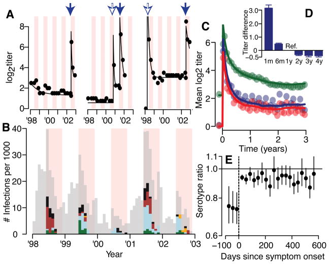
To track the evolution of an individual’s measured antibody titers (Figure 1A), we place titers on an adjusted log₂ scale (titers of 1:10 are given a value of 1, 1:20 of value of 2 etc.). There were 274 detected symptomatic DENV infections (Figure 1B); 62 were hospitalized (23%), 36 with dengue hemorrhagic fever (DHF) (13%). For those where the infecting serotype is known (79% of cases through PCR, Table S1), we observe a sharp rise and subsequent decay in log₂-titers following symptom onset (Figure 1C–D). The mean log₂-titer to the infecting serotype was 0.79 (95% CI: 0.74–0.84) times the log₂-titer to the non-infecting serotype in the three months prior to symptom onset compared to 0.94 (95% CI: 0.93–0.96) times in the six months after symptom onset (Figure 1E). As 86% of symptomatic infections had detectable titers to at least one serotype prior to infection, the higher antibody titer to non-infecting serotypes likely captures responses to prior infections¹⁰.

Figure 1. Titer responses following infection.

(A) Measured (dots) and model fit (lines) for three example individuals. Each dot represents the mean titer across the four serotypes. The pink shaded regions are periods of active surveillance. The solid blue arrows represent confirmed symptomatic dengue infections. The open blue arrows represent estimates of timing of subclinical infections from an augmented dataset. During the active surveillance windows, these augmented infections represent subclinical infections whereas outside the surveillance window, it is unknown if the individual had symptoms. (B) Serotype distribution of PCR confirmed symptomatic infections (DENV1 – green, DENV2 - blue, DENV3 - maroon, DENV4 – orange, unknown serotype – black). The grey bars represent the estimated distribution of infections not detected from active surveillance. The periods of active surveillance are in pink (5.5 months per year). (C) Model fit (lines) and observed (dots) titers pre and post infection for primary infections (infecting serotype in blue, non-infecting serotypes in red) and post-primary infections (green). (D) Mean difference between observed log2-titer at different time points following infection with that at 1 year for all augmented and observed infections (average of 1,421 total infections across 100 reconstructed datasets) with 95% confidence intervals. (E) Titer ratio of the infecting to the mean of the three non-infecting serotypes before and after symptom onset with 95% confidence intervals for the 217 individuals with symptomatic infections where infecting serotype detected (N=3,366 total titer measurements).

We reconstruct individuals’ antibody trajectories by assuming that infection leads to a rise in titers that subsequently decays exponentially¹¹. We also explore biphasic responses (Extended Data Figure 1). We allow for variability in antibody kinetics across individuals and infections, and for differential rises for the infecting versus the non-infecting serotypes for primary infections but undifferentiated responses for subsequent infections. We use data augmentation techniques to impute undetected infections (subclinical infections during active surveillance or unknown symptom status outside the surveillance windows) and to identify the serotype for undetected primary infections³. Instead of relying on fixed cutoffs to identify infections, data augmentation allows us to incorporate uncertainty in the existence, timing and serotype of unobserved infection events and therefore probabilistically assess whether differences in measured titers are due to infections or assay variability.

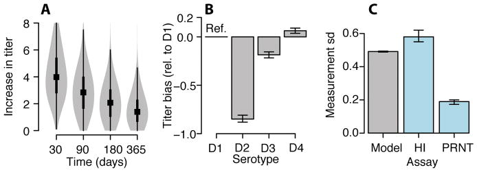
We find that following post-primary infection there is a mean 5.8 (95% CI: 5.6–5.9) rise in log₂-titers across serotypes, which declines by 76% after one year. For primary infections (i.e., individuals without detectable titers prior to infection) the mean log₂-titer rise is 7.6 (95% CI: 7.4–7.8) for the infecting serotype and 6.6 for the non-infecting serotypes (95% CI: 6.4–6.7). The similarity of titers of infecting and non-infecting serotypes coupled with assay variability suggests that in a clinical setting individual HI measurements cannot reliably determine the infecting serotype. We find that titers largely stabilize one year after infection to a set-point (the ‘set-point antibody load’) (Figure 1D). There is significant variability between infections: the interquartile range of the log₂-titer rise one year after infection is 0.7–2.2 across all infections (Extended Data Figure 2A). We find that even after accounting for historic infection status, measured DENV-2 titers are systematically lower than other serotypes (0.85 lower than DENV1) (Extended Data Figure 2B, Table S2), which could point to technical considerations of the DENV2 assay or inherent differences in immune responses to DENV2. We estimate the measurement error in the HI assay (i.e., the standard deviation in any reading) as 0.49 (95% CI: 0.49–0.50), which is similar with that empirically estimated using repeated testing on the same serum and 2.6 times error estimates for the plaque reduction neutralization test (PRNT) (Extended Data Figure 2C)¹². Despite the variability in individual readings, as we use many readings from four serotypes for each participant and titers appear to behave in a stable and predictable manner, we can nevertheless make robust inferences when considering the ensemble of the measurements.

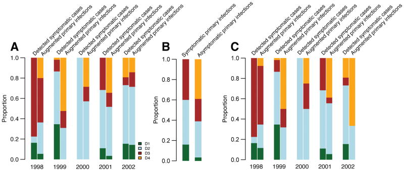
We probabilistically identify 1,149 undetected infections (95% range across model iterations: 1,135–1,163), of which 507 (494–520) occurred during active surveillance periods and were therefore subclinical (Figure 1B). Overall, we estimate 35% of infections are symptomatic (95% CI: 34–36). The temporal distribution of subclinical infections was correlated with that of symptomatic infections (Pearson correlation 0.78, 95% CI: 0.70–0.84). Using augmented primary infections where we could confidently assign the infecting serotype (same serotype implicated by >50% of iterations), we find that 34% of undetected primary infections (and 39% of subclinicial primary infections) were due to DENV-4, compared to only 3% of all symptomatic infections (none of which were primary infections) (Extended Data Figure 3A–B). We find consistent results using a more stringent cutoff to assign the infecting serotype (Extended Data Figure 3C). These findings are consistent with a reduced risk of disease from DENV-4 compared to other serotypes resulting in a largely silent DENV-4 epidemic. This is supported by a phylogenetic analysis that found DENV-4 was widespread in Thailand throughout this period (Figure S4 in Salje et al.,¹³). This suggests the serotype distributions from hospital-based or community-based surveillance may not be representative of infections in the population and supports previous evidence that the transmissibility of a serotype can be delinked from the propensity to cause symptomatic and/or severe disease^14,15. Further they imply that factors that contribute to transmission potential (e.g., viral replication, peak titers or infection length) are not predictive of adverse outcomes¹⁶.

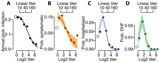
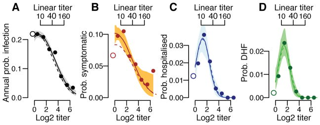
We find that the underlying probability of infection and the probability of developing disease are strongly linked to the mean antibody titer at the time of exposure. Overall, an individual’s annual risk of infection was 17%, varying from 21% for individuals with mean measured log₂-titers <2, to 16% for those with log₂-titers of 2–3 and 11% for those with log₂-titers of >3 (Figure 2A). Using logistic regression, we find that for log₂-titers >2, each unit increase in log₂-titers is associated with a 0.71 times relative risk of infection (95% CI: 0.67–0.76). The annual probability of having a symptomatic infection varies from 6.4% (95% CI: 4.9–8.4) for primary infections to 8.4% (95% CI: 7.8–9.1) for individuals with pre-existing log₂-titers ≤3 (≤1:40 on a linear scale) and 4.0% (95% CI: 3.0–5.0) for those with log₂-titers >3 (Figure 2B). The annual probability of being hospitalized during a primary infection was 1.2% (95% CI: 0.5–2.1), compared to 2.4% (95% CI: 2.1–2.7) during a subsequent infection for those with pre-existing log₂-titers ≤3 and 0.3% for those with log₂-titers >3 (95% CI: 0.09–0.6) (Figure 2C). Even more stark was the risk for developing DHF, which ranged from 0.2% (95% CI: 0.0–0.6) for primary infections compared to 1.5% (95% CI: 1.3–1.7) for subsequent infections in those with log₂-titers ≤3 and 0.0% for log₂-titers >3 (95% CI: 0.0–0.4) (Figure 2D). Within this study population, an average of 54% of the population had detectable log₂-titers of ≤3 at any time. Time-varying cox proportional hazards models that specifically account for the dependence of titer observations within individuals gave similar results (Extended Data Figure 4)¹⁷. Using log2-titers to probabilistically identify the cohort participants with detectable titers that will develop DHF has an AUC of 0.66 (Extended Data Figure 5).

Figure 2. Probability of infection and disease as a function of titer.

Annualized probability of (A) infection, (B) developing any symptoms, (C) being hospitalized and (D) developing DHF as a function of the mean measured antibody titer across all serotypes at the time of exposure across all study subjects (N=3,451). The open circles on the left represent primary infections (i.e., those with no detectable titers to any serotype prior to exposure). The shaded regions represent 95% bootstrap confidence intervals.

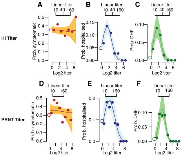
Considering only infected individuals, we observe no difference in the probability of subclinical infection by titer; however, the probability of hospitalization and DHF remains greatest in those with pre-existing log₂-titers of ≤3 (Extended Data Figure 6A–C). Only one individual with pre-infection log₂-titers >3 developed DHF during surveillance compared to 146 who did not but had titers at infection within the same range. This suggests that in the event that infection takes place, antibodies are not protective of developing symptoms per se but, conversely, are associated with the development of severe disease. We observe no difference in the risk of disease given infection across years (Table S3) or age (Table S4). Other studies are needed to see if younger age groups than those included here nevertheless have increased risk. PRNTs form the basis of current discussions on immune correlates. Among those infected, individuals with detectable PRNT log₂-titers of ≤4.5 (equivalent to approximately ≤1:100) have 7.5 times (95%CI: 2.4–11.6) increased risk of DHF compared to previously naïve individuals, compared to 0.0 times for those with higher titers (Extended Data Figure 6D–F). Cross-reactive titers that result from exposure to non-DENV flaviviruses such as Japanese encephalitis and Zika may be included in these risk estimates.

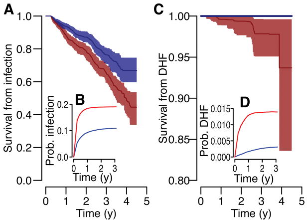
Our findings suggest that post-infection set-point antibody loads appear important to determining individual infection and disease risk. Post infection, we estimate the daily probability of a subsequent infection and the development of DHF disease as a function of titer dynamics. We demonstrate that the probability of both infection and disease stabilizes after 1y (Figure 3). Based on our observation in Figure 2 that individuals with detectable titers of ≤3 had increased risk of infection and disease, we explored the temporal evolution of risk following infection for those with setpoint antibody loads (i.e., the titer at 1y following infection) above and below this threshold. At 1 year, we observe a 2.1 times increased risk of infection (irrespective of disease outcome) for those with setpoint antibody loads of ≤3 compared to those with greater antibody loads and an 8.9 times increased risk of infection that leads to DHF. Overall, we find that three years following infection 34% of individuals with setpoint antibody loads of ≤3 suffer a subsequent infection, irrespective of severity (95% CI: 33%–35%) compared to 23% for those with greater loads (95%CI: 20%–26%). After this delay 3.5% of individuals with setpoint loads of ≤3 develop DHF disease (2.4%–4.4%) compared to none in those with higher loads. The apparent stability of setpoint antibody loads points to an ability to assess an individual’s long-term risk.

Figure 3. Risk of subsequent infection and disease following an infection event (from average of 1,420 infections across 100 reconstructed datasets).

The probability of survival from subsequent infection (irrespective of disease outcome (A) and that lead to DHF (C)) as calculated from Kaplan-Meier for those with setpoint antibody titers of ≤3 (red) and >3 (blue) with 95% confidence intervals. The annualized probability of a subsequent infection (irrespective of disease outcome (B) and that lead to DHF (D)) at different time points following infection for those with setpoint antibody titers of ≤3 (red) and >3 (blue).

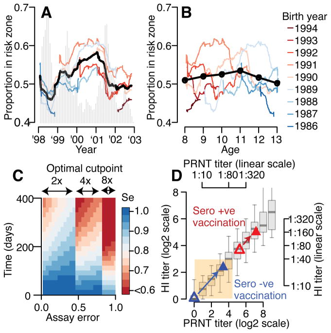
Our findings are consistent with low titers generated by some candidate vaccines in previously naïve individuals ‘priming’ individuals for severe disease upon their first exposure¹⁸. A hypothesis supported by previous evidence that primary infections in infants with maternal antibodies and secondary infections in older individuals are associated with severe disease^19,20. Further, a Nicaraguan study found elevated risk of severe disease for those with low iELISA titers at prior annual blood draws⁹. Previously naïve individuals given the Dengvaxia vaccine had mean PRNT titers within our risk window (Figure 4D)²¹. Further work is required to understand whether immunity acquired from vaccination and natural infection are qualitatively similar and whether the risk window described here is relevant for vaccine recipients. T-cell immunity, which is not captured by these assays, might compensate for antibody titers in this window. Vaccine studies should carefully assess the criteria used to define seroconversion, and how titers correlate with disease risk over time. Our work suggests that previously used criteria (PRNT titer >1:10) do not adequately correlate with reduction in disease risk and suggest that HI titers >1:40 or PRNT titers of >1:100 may provide a starting point for any vaccine in identifying a targeted neutralizing antibody response. Placebo arm data from the Dengvaxia vaccine trials also suggests higher PRNT titers are linked to protection ²². The targeted vaccination of individuals that have pre-existing antibody titers within our zone may be a viable approach to minimize the public health burden from dengue by moving individuals away from the risk window (Figure 4D). Even in an endemic setting such as our cohort, there is considerable temporal variability in the serological status of 9y individuals (Extended Data Figure 7) suggesting that the current WHO guidance surrounding Dengvaxia or similar guidance based on serostatus at vaccination will have to carefully consider this variation or specifically screen individuals.

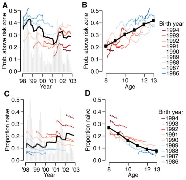
Figure 4. Evolution of population risk, implications for vaccine and cohort design.

(A) Proportion of study participants who have titers in risk zone (defined detectable log2-titers ≤3) over the study period for different birth-cohorts (colored lines) and overall (black). The epidemic curve of all infections is in grey. (B) Proportion of study participants with titers in risk-zone as a function of age for different birth-cohorts (colored lines) and overall (black). (C) Performance of current assay testing protocol where infection events are defined as a rise above a cut-point in any serotype across two blood draws. (D) Relationship between PRNT titer and HI titer where both assays were performed (N=1,771 samples). The boxplots show 2.5, 25, 75 and 97.5 quantiles as well as the mean. Superimposed are the results from the Denvaxia vaccine for previously seronaive (blue) and seropositive (red) prior (open symbols) and post (filled symbols) vaccination.

Our approach allows us to consider wider problems concerning drivers of dengue epidemiology. The assumption that population-wide immunity varies in time and dictates multi-annual dynamics of dengue pervades the literature and dominants current hypotheses about what drives large outbreaks of dengue in particular settings^18,23–26. More generally, the idea that temporally varying population immunity drives temporal dynamics of pathogens pervades infectious disease epidemiology^27–29. However, quantitative evidence that any population varies in dengue immune status over time is largely lacking, as is a link between the immune status of a population and the risk of epidemics in empirical data. Here, though we have only a short time series, we show that underlying heterogeneity in the size of annual epidemics mean the risk of having titers within-the risk zone for different birth-cohorts are more correlated by epidemic time-point (Figure 4A, mean correlation of 0.70) than by age (Figure 4B, mean correlation of 0.23). While both the probabilities of being naïve and having log₂-titers above the risk-zone are correlated with age, there also exist strong birth-cohort effects (Extended Data Figure 7). For example, among 9 year olds, we observe up to a two-fold difference in the probability of being naive, depending on the year of the study.

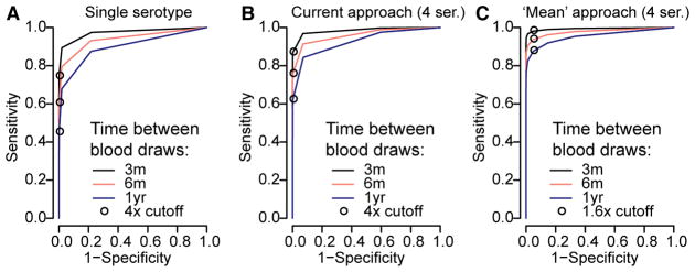
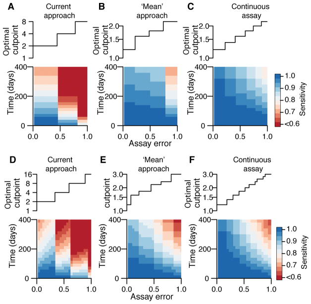
Finally, our results can guide the design of cohort studies aiming to characterize transmission. Studies typically use a four-fold rise in titers against any serotype as evidence of infection, regardless of the timing of sample collection. Using our titer trajectories, we find that if blood draws are every 90 days, a four-fold cut-point on measured titers has a specificity of >99% and a sensitivity of 87% (Figure 4C, Extended Data Figure 8). The sensitivity is reduced to 77% when blood is taken every six months and 62% when blood is taken annually, although it may be higher in seasonal settings when samples are taken at the season’s end. Using an alternative approach that uses the mean titer across the four serotypes and a 1.6-fold cut-point, the sensitivity of the assay improves to 96% when samples are taken every six months and to 90% for annual bleeds (specificity >95%) (Extended Data Figure 9). We provide the optimum cut-point and estimated sensitivity for these approaches and a theoretical one where titers are on a continuous scale (such as PRNT) and where a minimum specificity of >99% is required (Extended Data Figure 9).

We demonstrate through simulation that our framework can recover the true number of subclinical infections and parameters when only 30% of infections are symptomatic (Table S5). Our approach is also robust to a scenario where there are differential rises in titers for symptomatic and non-symptomatic infections (Table S6) and where we incorporate school specific force of infection parameters (Table S7). In addition, we find the timing (Extended Data Figure 10A) and the serotype (Extended Data Figure 10B) of undetected infections cluster in the same locations as symptomatic infections. This provides strong support of our modeling framework by suggesting that the model can correctly identify spatio-temporal clustering of otherwise undetected infections. These findings also support focal transmission, irrespective of disease outcome^13,30,31. The approach presented here will be applicable across disease systems where longitudinal titer data exists, allowing a wide range of insights into fundamental questions of disease ecology and risk.

Methods

1. Cohort study design

Individuals attending 12 different schools in Kamphaeng Phet district, a rural region of Northern Thailand were recruited into a dengue cohort study that ran between 1998 and 2003 as previously described³². All individuals were between seven and 13 years old. Blood samples were taken four times a year (in January, June, August and November) with an average of 91 days between blood draws. In addition, from the start of June to mid November each year, active surveillance was conducted through school-based surveillance. Children who missed school due to febrile illness had additional acute and convalescent blood draws. Dengue infection was confirmed using RT-PCR on the acute sample, with the infecting serotype also recorded or through antibody detection (IgM ELISA values >40 or HI rises of over four times between acute and convalescent blood draws), in which case the infecting serotype was not known. The date of symptom onset, whether or not the child was hospitalized and whether or not they developed DHF was also recorded. Note that the cohort study was conducted prior to 2009 when the WHO provided new guidance of the characterization of different levels of dengue severity.

2. Antibody measurements

For each individual’s blood draw, antibody titers to each of DENV1, DENV2, DENV3, and DENV4 were measured using a hemagglutination inhibition assay. The following two-fold dilutions were used: 1:10, 1:20, 1:40, 1:80, 1:160, 1:320, 1:640, 1:1280 and 1:2560. We translated each titer onto a log₂ scale such that 1:10 was given a value of 1, 1:20 of value of 2 and so on. Undetectable titers (those with a titer of <1:10) were given a value of 0. For a subset of 800 individuals, 1,771 samples were also tested using plaque reduction neutralization tests (PRNTs). These samples were either paired samples from individuals with symptomatic confirmed infection with one sample taken from a time point prior to symptom onset and one sample from post symptom onset (N=75 pairs) or randomly chosen sequential blood samples from individuals without a detected symptomatic infection between the blood draws.

3. Characterizing how titers change following symptomatic infection

We can understand how titers to both the infecting serotype and to non-infecting serotypes change over time prior to and following symptom onset. For all individuals that experienced a symptomatic illness where the infecting serotype was identified, we identify all titer measurements within each 10-day window from 100 days prior to symptom onset to 600 days post symptom onset. For each window, we calculate the mean titer to the infecting serotype and the average mean titer to the other three serotypes across all individuals that had a blood draw within that window.

4. Modeling the dynamics of dengue antibody titers

Previous efforts in malaria have used hidden Markov models to include undetected infections in estimates of the transmission intensity using presence/absence of specific antibodies in longitudinal data³³. While these efforts are able to improve estimates on the force of infection within a community compared to using symptomatic individuals, they do not incorporate the changing dynamics of antibody titers over time. By specifically including titer dynamics, we can help understand a wide range of issues, including assay error, measures of protection and risk and cohort design.

4.1. Notation

We consider an individual i. We denote $n_i^I(t)$ the number of times the individual was infected prior to time t. Each dengue infection of individual i is labeled by the index $\psi =\mathit{1}\dots n_i^I(t)$. We denote ${\tau }_{i,\psi }^I$ the time of infection number ψ of individual i and s_{i, ψ} the infecting serotype of infection number ψ of individual i. The history of infection (i.e., the timing and serotype of all infections since birth) of individual i up to time t is labeled H_i(t). We denote $N_i^A$ the total number of times the individual had blood taken during the study. Each blood draw of individual i is labeled by the index $\pi =\mathit{1}\dots N_i^A$. We denote ${\tau }_{i,\pi }^A$ the time of blood draw π for individual i. We denote A_{i, s, π} the true antibody titer (see Section 4.3) and $A_{i,s,\pi }^{\ast }$ the measured antibody titer for individual i for serotype s at blood draw π. Λ_i(t) represents the cumulative force of infection exerted on individual i prior to time t. The parameter vector is denoted by θ.

4.2. Hierarchical structure of the model

We can break down the probability of a measured antibody titer into three components:

$$\begin{gathered} P\left(A_{i,s,\pi =k}^{\ast }\right|A_{i,s,\pi =k}) \\ ·P\left(A_{i,s,\pi =k}|{\tau }_{i,\psi =1}^I,\dots {\tau }_{i,\psi =n_i^I(t={\tau }_{i,\pi =k}^A)}^I,s_{i,\psi =1},\dots s_{i,\psi =n_i^I(t={\tau }_{i,\pi =k}^A)},A_{i,s,\pi =1},\dots A_{i,s,\pi =k-1}\right) \\ ·P(H_i(t={\tau }_{i,\pi =k}^A)\left|{\{\lambda \}}_t\right) \end{gathered}$$

The first part represents the ‘measurement model’, the second part the ‘antibody dynamics model’ and the third part the ‘infection model’.

4.3. Measurement model

We model the underlying antibody levels on a continuous scale, however, the hemagglutination inhibition assay is a discrete assay, such that in a situation of no measurement error or systematic biases, a true antibody titer between any two dilutions would be measured as the lower of the two dilutions. So for example, a true titer of 2.7 would be measured as 2 (assuming there are dilutions performed at 0,1,2,3…). In addition, there is also likely to exist measurement error and there may be underlying differences by serotype (i.e., serotype-specific biases) in the assay that will impact all measurements of antibodies against a particular serotype. We consider a ‘true titer’ to represent the underlying (but unmeasured) titer on a continuous scale. A ‘measured titer’ is the value that is actually measured by the assay. Conditional on an individual’s history of infection, we assume independence between the measurements of the different serotypes. This seems a reasonable assumption as assays are performed separately for each serotype. The probability of the measured titers, $A_{i,s,\pi =k}^{\ast }$ is:

$$P\left(A_{i,s,k}^{\ast }\right|A_{i,s,k})={\int }_{A_{i,s,k}^{\ast }}^{A_{i,s,k}^{\ast }+1}f(u)du$$

where f(u) is the density for a normal distribution with mean A_{i, s, k} + χ_s and a standard deviation parameter, σ. Where:

$$\begin{gathered} {\chi }_s=0\text{if}s=\mathit{DENV}\mathit{1} \\ {\chi }_s={\chi }_2\text{if}s=\mathit{DENV}\mathit{2} \\ {\chi }_s={\chi }_3\text{if}s=\mathit{DENV}\mathit{3} \\ {\chi }_s={\chi }_4\text{if}s=\mathit{DENV}\mathit{4} \end{gathered}$$

4.4. Antibody dynamics model

If an individual i was never infected by dengue, we assume they will have titers of 0 against the four serotypes (this assumes any maternal antibodies have disappeared and there is no impact of infections by other flaviviruses). At each time point that the individual becomes infected, their antibody titers will rise. We assume that the rise can be broken down into a permanent increase (representing antibodies that will continue to circulate, long after the infection has passed) and a temporary increase (representing the short-lived antibodies generated upon infection).

4.4.1. Permanent rise in titers

The permanent rise in titers Q_{i, s}(ψ), for serotype s from infection number ψ in individual i is modeled as:

$$Q_{i,s}(\psi )={\omega }_{i,\psi }·K(\psi ,s)$$

where ω_{i, τ} is a random effect that is gamma distributed with mean parameter ω_m and variance parameter ω_v and K(ψ, s) allows differential antibody response by serotype for primary infections: K(ψ, s) = η if it is a primary infection (i.e., ψ=1) and s is the infecting serotype; K(ψ, s) = 1 otherwise.

4.4.2. Temporary rise in titers

We assume that temporary antibody responses will decay exponentially over time:

$$R_{i,s}(t\mid H_i(t))={\gamma }_{i,\psi =n_i^I(t)}·exp\left(-\left(t-{\tau }_{i,\psi =n_i^I(t)}^I\right)·{\delta }_{i,\psi =n_i^I(t)}\right)·K(\psi =n_i^I(t),s)$$

where ${\gamma }_{i,\psi =n_i^I(t)}$ is a random effect that captures the instantaneous rise in temporary antibody titers following the most recent infection (infection $n_i^I(t)$) prior to time t that comes from a gamma distribution with mean parameter γ_m and variance parameter γ_v; ${\delta }_{i,\psi =n_i^I(t)}$ is the rate of decay of the temporary antibodies and comes from a gamma distribution with mean parameter δ_m and variance parameter δ_v. As with the permanent rise in titers, $K(\psi =n_i^I(t),s)$ allows differential antibody responses for primary infections: K(ψ, s) = η if it is a primary infection (i.e., ψ=1) and s is the infecting serotype; K(ψ, s) = 1 otherwise. Additional work is needed to understand if alternative functional forms for the rise and decay in antibody titers may further refine how antibodies behave following infection.

4.4.3. Overall trajectory of antibody titers

Under these assumptions, and an additional linearity assumption that the temporary and permanent rises are additive, antibody titers at blood draw k for serotype s in individual i is:

$$A_{i,s,\pi ,k}=Q_{i,s}(\psi =1)+\cdots +Q_{i,s}\left(\psi =n_i^I(t={\tau }_{i,\pi =k}^A)\right)+R_{i,s}\left(t={\tau }_{i,\pi =1}^A\mid H_i(t={\tau }_{i,\pi =k}^A)\right)+\cdots +R_{i,s}\left(t={\tau }_{i,\pi =k}^A\mid H_i(t={\tau }_{i,\pi =k}^A)\right)$$

4.5. Infection history model

We first assume that both the number of infections and the timing of infections are known. This assumption will subsequently be relaxed. We assume that each individual can get infected up to four times (once by each serotype). An individual’s history of infection depends on seasonality in dengue transmission and differences in the force of infection across years. For a particular time t, the force of infection is assumed to be:

$$\lambda (t)=\overline{\lambda }·{\beta }_{\mid t\mid }·\left(1+\delta ·cos\left(\zeta +\frac{2\pi t}{365}\right)\right)$$

where λ̄ is a parameter that represents the mean daily force of infection in 1998 (the first year of the study) and β_[t] is the mean force of infection in year |t| as compared to that in 1998.

For an individual i, the contribution to the likelihood for periods prior to any infection the probability of their infection history can be broken down into periods of infection and periods without infection. Individuals only contribute to the likelihood during their time in the study.

For each infection that occurs at time t, the contribution to the likelihood is:

$$log(1-exp\left(-\lambda (t)\right))$$

For each individual, each day during which no infection occurs, the contribution to the likelihood in respect of serotype s is:

exp(−λ(t))	- where more than 90 days have passed since an infection by any serotype and the individual has not previously been infected by serotype s
0	- otherwise, including periods when the individual is not part of the study

The presence of the 90-day window where no infection can take place avoids there being more than one infection event between two blood draws. This period is substantially shorter than the estimated period of cross-protection between serotypes of 2 years³⁴.

4.5.1. Context of full observation

In the context of full observation, the probability of the history of infection for individual i can be given as:

$$P\left(H_i(t={\tau }_{i,\pi =k}^A)|{\{\lambda \}}_t\right)=\prod _{k=1}^{n_i^I(T_i)}exp\left(-{\int }_{{\tau }_{i,k-1}^I}^{{\tau }_{i,k}^I}\lambda (u)du\right)(1-exp(-\lambda ({\tau }_{i,k}^I)))·\mathit{exp}\left(-{\int }_{{\tau }_{i,n_i^I(T_i)}^I}^{T_i}\lambda (u)du\right)$$

where ${\tau }_{i,0}^I$ represents the time of birth and T_i the time point at which individual i leaves the study (defined as the day of their final blood draw). We assume the same λ(t) for all serotypes.

4.6. Situation of imperfect observation

In practice, we do not know the infection history of all individuals. Many infections will have occurred before individuals entered the study. In addition, there are likely to be many subclinical infections that would not have been detected through active surveillance. In addition, active surveillance only operated 5.5 months of every year. Infections outside these periods would also have been missed (irrespective of symptoms).

4.6.1. Unobserved infections prior to recruitment

For the infection history of individuals before they enter into the study, we estimate a baseline titer A_{i, s}(t₀) that represents the titer to serotype s one year prior to the first blood draw. As we assume linearity, such that the temporary and permanent titers of successive historic infections sum up to give the titer at a moment in time, this estimated baseline titer allows us to incorporate the impact of historic infection events up one year prior to enrollment but means we do not need to infer infection events before that time. Individuals that are naïve at baseline (defined as those with no measured titers to any serotype at the first blood draw) are given a baseline titer of 0. For an individual with no infection events during the study period, A_{i, s}(t)= _{i, s}(t₀) for all t.

4.6.2. Use of data augmentation for undetected infections or serotype during study

In the context of full observation during the study period, each individual would have the serotype and time from each infection, {s_i,ψ, τ_i,ψ}, known. In the setting of undetected infections or detected infections but infecting serotype is unknown (such as when symptomatic infections are only detected through IgM ELISA and therefore the serotype is unknown), we can use a Bayesian data augmentation framework. In this framework, the incompletely observed {s_i,ψ, τ_ι,ψ} pairs are incorporated and considered as nuisance parameters. The joint posterior distribution of the parameters and the augmented data is explored via reversible-jump MCMC sampling.

If we call $\mathrm{y}={\left\{{\mathrm{s}}_{i,\psi }^{\ast },{\tau }_{i,\psi }^{\ast }\right\}}_{i=1,\mathrm{..}N,\psi =1,\dots n_i^{\ast }(t=\infty )}$ the observed data, z = {s_{i, ψ, τi, ψ}}_{i=1, … N, ψ = 1, … ni(t=∞)} the full data (made up of the observed data and the augmented data), the joint posterior is:

$$\mathrm{P}(\mathrm{z},\mathrm{\theta }\mid \mathrm{y})\propto \mathrm{P}(\mathrm{y}\mid \mathrm{z})·\mathrm{P}(\mathrm{z}\mid \mathrm{\theta })·\mathrm{P}(\mathrm{\theta })$$

P(y|z) represents the observation model, P(z|θ) is the titer model outlined above and P(θ) gives the prior distribution of the parameters.

The observation model makes sure that the augmented datasets are consistent with the observed data by having a value of 1 (if consistent) or 0 (if inconsistent). Consistent augmented data have the following characteristics:

1. No individual is infected during the study period by the same serotype more than once

2. No individual is infected more than once during a 90 day period

Note that, as DENV-titer responses to non-DENV flaviviruses such as Zika and Japanese encephalitis are likely to be smaller that to DENV infections, such exposures are unlikely to be detected by our model and incorporated as measurement uncertainty instead.

4.6.3. Date of symptom onset, date of infection and date of titer rise

For all detected (symptomatic) infections, we only detect the date of symptom onset and not the date of infection. To obtain the day of infection for symptomatic cases we subtract a fixed period of 7 days from the day of symptom onset, representing the median incubation period for dengue³⁵. Titers may also not rise on the day of symptom onset (due to recall bias in when symptoms started or individual level variability). For symptomatic infections, we approximate the true, unobserved day of titer rise using augmentation, where we define consistent augmented data for which the day of titer rise is within ten days of the reported date of symptom onset. For augmented (undetected) infections, we assume that the day of titer rise following infection always occurs 11 days after the day of infection, which represents an approximate estimate of the time between infection and day of titer rise: calculated as the sum of the median incubation period for dengue (seven days) and the median time between symptom onset and titer rise for the detected infections (four days).

4.6.4. Impact of uneven data collection through time

This cohort used a rolling recruitment approach, which maintained an approximately constant sized population and constitutes an important strength compared to cohorts whose size may be strongly affected by participant dropout. As individuals only contributed to the likelihood for their period of inclusion in the cohort and dropout is not expected to depend on the history of infection, we do not expect that the turnover of participants in the cohort will bias parameter estimates. This was demonstrated in a simulation study where we were able to recover true parameters for a simulated cohort with a similar design (see Section 4.8).

4.6.5. Prior distributions

We use a log-normal distribution with log-mean 0 and log-variance of 1 for the parameters: mean and variance in the permanent rise in log₂-titers (ω_m, ω_v), mean and variance in the temporary rise in log₂-titers (γ_m, γ_v), mean and variance in the decay in log₂-titers per day (δ_m, δ_v), difference in rise for infecting vs. non infecting serotype (primary infection only) (η), measurement error (σ), DENV2-4 bias (χ_2, χ_3, χ₄), daily force of infection in 1998 per serotype (λ), relative force of infections versus 1998 for 1997 (β₀) and 1999–2002 (β₂-β₅) and the two seasonality parameters (δ and ζ).

4.7. Estimation using MCMC

We develop a Markov chain Monte Carlo approach to explore the joint posterior distribution of parameters and the augmented data with the following steps:

1. Metropolis-Hastings update for the model parameters θ in turn with the updates performed on a logarithmic scale. The step size of the proposals was adjusted to obtain an acceptance probability of 20–30%. As the vast majority of infections are undetected, when updating the six parameters that determine the rise and decay of antibodies (namely ω_m, ω_v, δ_m, δ_v, γ_m, γ_v,), we calculate the likelihood using only the titers from one month prior to and year post the symptomatic (and therefore detected) infections. This approach assumes that the rise and fall in titers from all infections come from the same distributions, irrespective of symptom status. More work is needed to understand if whether or not an infection leads to symptoms changes the titer dynamics following that infection.

2. For the symptomatic cases, as the day of titer rise may not fall exactly at the recorded day of symptom onset we use an independence sampler to update the day of titer rise. At each iteration, the day of the titer rise was updated for 100 randomly chosen symptomatic infections. Candidate values were chosen using a uniform distribution between 10 days prior to and 10 days post the recorded date of symptom onset.

3. Independence sampler for the identity of the infecting serotype for the 62 symptomatic infections where the serotype was not identified. At each iteration, the serotype for each of these infections is updated with equal probability across the four serotypes.

4. Independence sampler for the identity of the infecting serotype for the undetected infections. At each iteration, the serotype for 500 randomly chosen undetected infections is updated with equal probability across the four serotypes.

5. Independence sampler for the dates of titer rise for undetected infections. At each iteration, the day of infection is updated for 1000 randomly chosen undetected infections. For each infection, the proposal is a uniform distribution between one year prior to entry into the study and the day of the final blood draw.

6. Independence sampler for the baseline titers for each individual. At each iteration, the baseline titer for one serotype is updated for 1000 randomly chosen individuals. The proposal distribution is a random uniform distribution between 0 and 10. All individuals that are naïve at baseline (i.e., those with no titers to any serotype at the first blood draw) are forced to have a baseline titer to 0 for all four serotypes.

7. Reversible jump –MCMC to add/remove unobserved infection events. As H_i(t_j) is unobserved, we use a Bayesian data augmentation approach that treats it as a nuisance parameter. Rather than attempting to definitively identify whether an infection occurred or not, these approaches allow us to incorporate the uncertainty of the presence and timing of these events. We use reversible jump MCMC (RJ-MCMC) to add and remove infection events. Each step to add undetected infections proceeds as follows:

   1. Randomly draw individual.

   2. Draw a candidate date for the infection event using a uniform distribution from 1 year prior to their first blood draw to the day of their final blood draw.

   3. Draw a candidate serotype of infection with the probability of each serotype being 0.25.

   4. Update the number, date and serotype of infections for that individual.

   For the removal of undetected infections, we use a similar approach:

   1. Randomly draw individual.

   2. If that individual has undetected infections, randomly select one of their infections with equal probability (if they have no infections move to the next individual).

   3. Update the number, date and serotype of infections for that individual by removing that infection.

4.8. Evaluation of model using simulated data

In order to evaluate the ability of the model to accurately estimate the parameters in a scenario when only a minority of infections are observed, we use the same modelling framework on a random subset of 1,000 individuals from the study with subsequent changes in titers, We include the actual start date and the end date for these individuals (i.e., when they entered and left the cohort). We simulate infections in these individuals based on known parameters. We then randomly ‘unobserve’ 70% of infections to reflect undetected infections. We then estimate the parameters using our framework and compare them to the underlying true parameters.

4.9. Sensitivity analysis using school-specific force of infection parameters

The force of infection exerted on individuals may differ across schools, resulting in non-independence between individuals attending the same school. To assess the impact of any such correlation on our parameters, we performed a sensitivity analysis where we included a separate force of infection parameter for each school. In this model the force of infection exerted on an individual that attends school sch is:

$$\lambda (t,\mathit{sch})=\overline{\lambda }·{\beta }_{\mid t\mid }·{\beta }_{\mid \mathit{sch}\mid }·\left(1+\delta ·cos\left(\zeta +\frac{2\pi t}{365}\right)\right)$$

where λ̄ is a parameter that represents the mean daily force of infection in 1998 in school 1, β_[t] is the mean force of infection in year |t| as compared to that in 1998 and β_[sch] is the mean force of infection for school sch as compared to school 1.

4.10. Alternative functional forms for the decay in titers

Alternative functional forms for the decay in antibody titers exist. In particular, biphasic models that model both short-term antibody decay and longer-term antibody decay with different exponential decay rates have been shown to work well in other systems, such as malaria³⁶. The biphiasic form is captured by:

$${\text{Titer}}_{\mathrm{t}}={\theta }_1·({\theta }_2·exp(-{\theta }_{3}t)+(1-{\theta }_2)·exp(-{\theta }_{4}t))$$

where θ₁, θ₂, θ₃ and θ₄ capture the decay of the titers. To explore whether this biphasic form may further refine how antibodies behave following infection here, we fitted both exponential decay and biphasic models to the observed infections using the observed titers following detected PCR-confirmed infections and the dates of symptom onset. We found largely consistent results in the two models (Extended Data Figure 1). As exponential decay is the more parsimonious model, we retained this form for the final analysis. Nevertheless, structural uncertainty in the model used for the analysis remains, which will not be represented within the confidence intervals for the parameters.

4.10. Estimation of impact on titers on infection and disease

4.10.1. Estimation of impact of mean titers on infection

We use the augmented times and serotypes of infection from 100 model iterations to reconstruct the antibody titer trajectories for each individual. For each augmented dataset we extract the mean titer across all four serotypes for each day and whether they got infected in the following day or not. Person-time in individuals who were considered not susceptible (i.e., had been infected in the prior 90 days) was excluded. To explore the relationship between mean titer and the probability of infection we conducted logistic regression where we used a polynomial spline of order 2 for the mean titer (determined as the optimal model through comparison of different polynomial models by AIC). To account for sampling uncertainty, in each reconstructed dataset we use a bootstrap approach to sample all individuals with replacement and then re-perform the logistic regression each time. We present the mean and 95% confidence intervals from the resultant distribution of the logistic model estimates of the probability of infection for each titer obtained from across the model iterations.

4.10.2. Estimation of impact of mean titers on disease outcome

We explore the relationship between mean titer and the probability of having different disease outcomes. We consider three different outcomes: symptomatic infection (irrespective of severity), hospitalization and DHF. We use the same approach as in Section 4.9.1. but only consider titers during the active surveillance windows and whether or not individuals had an infection the following day that led to the outcome of interest. For each outcome, we conduct logistic regression where we use a polynomial spline of order 2 for the mean titer (consistently determined as the optimal model through comparison of different polynomial models by AIC). We use a bootstrap approach to sample all individuals with replacement and then re-perform the logistic regression each time and identified the mean and 95% confidence intervals from the resultant distribution for the estimates of the probability of having an infection that led to the outcome of interest for each titer obtained from across the model iterations.

4.10.3. Estimation of impact of mean titers on disease outcome, conditional on being infected

For those that became infected during the active surveillance windows, we fit logistic models to the mean titers and whether or not the disease outcome occurred. We looked at three outcomes: any symptomatic illness, hospitalization and DHF. For each of the three outcomes, we compare an intercept only model with models with a polynomial spline up to order 2. To account for sampling uncertainty, in each reconstructed dataset we use a bootstrap approach to sample all individuals who had an infection during the surveillance windows with replacement and then re-perform the logistic regression each time. We present the mean and 95% confidence intervals from the resultant distribution of the logistic model estimates of the probability of infection for each titer obtained from across the model iterations.

4.10.4. Estimation of impact of mean PRNT titers on disease outcome, conditional on being infected

PRNT titers are available for a subset of 1,771 blood draws. For those that became infected during the active surveillance windows and PRNT titers are available in the six months window prior to infection, we fit logistic models to these mean PRNT titers from that six-month time frame and whether or not the disease outcome occurred. We looked at three outcomes: any symptomatic illness, hospitalization and DHF. For each of the three outcomes of interest, we compare an intercept only model with models with a polynomial spline up to order 2. To account for sampling uncertainty, in each reconstructed dataset we use a bootstrap approach to sample all individuals who had an infection during the surveillance windows with replacement and then re-perform the logistic regression each time. To account for the fact that individuals and serum samples may not have been completely selected at random for PRNT testing (e.g., preferential testing of those with symptomatic disease), we adjusted our estimate for the probability of sampling conditional on the outcome of interest.

From the logistic regression described above, we can extract the probability of the outcome of interest given a particular PRNT titer and that a PRNT was conducted. Using Bayes rule we can write down:

$$P(\mathit{outcome}\mid \mathit{titer},\mathit{PRNT}\mathit{done})=\frac{P(\mathit{PRNT}\mathit{done}\mid \mathit{outcome},\mathit{titer})P(\mathit{outcome}\mid \mathit{titer})}{P(\mathit{PRNT}\mathit{done}\mid \mathit{titer})}$$

as the PRNT titer (or the HI titer) was not taken into account in the section process for choosing whether or not a PRNT was done, this becomes:

$$P(\mathit{outcome}\mid \mathit{titer},\mathit{PRNT}\mathit{done})=\frac{P(\mathit{PRNT}\mathit{done}\mid \mathit{outcome})P(\mathit{outcome}\mid \mathit{titer})}{P(\mathit{PRNT}\mathit{done})}$$

As we are interested in P(PRNT done|outcome), we can reorder this equation to:

$$P(\mathit{PRNT}\mathit{done}\mid \mathit{outcome})=\frac{P(\mathit{outcome}\mid \mathit{titer},\mathit{PRNT}\mathit{done})P(\mathit{PRNT}\mathit{done})}{P(\mathit{outcome}\mid \mathit{titer})}$$

We therefore multiply our logistic model outcomes by the following adjustment factor:

$$\mathit{adj}.\mathit{factor}=\frac{P(\mathit{PRNT}\mathit{done})}{P(\mathit{PRNT}\mathit{done}\mid \mathit{outcome})}$$

P(PRNT done) is calculated as the proportion of all infection events where a PRNT was conducted in the prior 6 months from the infection and P(PRNT done|outcome) is calculated as the proportion with the outcome of interest where PRNTs were conducted in the prior 6 months. We present the mean and 95% confidence intervals from the resultant distribution of the logistic model estimates of the probability of infection for each titer obtained from across the model iterations.

4.10.5. Estimation of impact of year and age on mean titers on disease outcome

We used a logistic regression approach to explore the impact of year of infection and the age at the time of infection. To explore the impact of year, we take each augmented dataset in turn and sample all the individuals with replacement to incorporate sampling uncertainty. We then regress the year of infection (as a categorical variable) on whether the outcome Y_{i, t} occurred:

$$\mathit{logit}\left(Y_{i,t}\right)={\beta }_0+{\beta }_1·{\mathit{Year}}_{i,t}$$

where Year_{i, t} is the year (1998, 1999, 2000, 2001 or 2002) within which day t occurred for individual i. We conducted separate regression where the outcome was an infection event (irrespective of whether the infection led to symptoms), symptomatic infection events (irrespective of disease severity), hospitalization and development of dengue hemorrhagic fever. For the last three models we only considered data during the active surveillance windows, as we do not know the symptom status of infections outside these windows. To explore the impact of age, we dichotomized the age of individuals as being less than or greater than 9 (the Sanofi Pasteur vaccine is not recommended for individuals under 9). We then performed the regression:

$$\mathit{logit}\left(Y_{i,t}\right)={\beta }_0+{\beta }_1·{\mathit{Age}}_{i,t}$$

where separate models for the same four outcomes, Y_{i, t}, were peformed. Finally, we built multivariable models that also accounted for mean titer using a polynomial of order 2:

$$\mathit{logit}\left(Y_{i,t}\right)={\beta }_0+{\beta }_1·{\mathit{Age}}_{i,t}+{\beta }_2·{\mathit{Titer}}_{i,t}+{\beta }_2·{\mathit{Titer}}_{i,t}^2$$

4.11. Impact of titer on outcome using cox proportional hazard models

In the context of small probabilities of an event occurring and short time intervals between readings, logistic regression will give consistent results with that from cox proportional hazards models that specifically takes the non-independence of titer observations from the same individuals into account¹⁷. To demonstrate the consistency of the two approaches we estimate the impact of titer on our four outcomes (infection, symptomatic infection, hospitalized infection and DHF infection) using a time-varying cox proportional hazards model, specifically incorporating clustering of observations by individual³⁷. We used 100 augmented datasets. For each augmented dataset we extract the mean titer across all four serotypes for each day and whether they got the outcome of interest in the following day or not. For the disease specific outcomes (any symptomatic disease, hospitalized infection and DHF infection), we only used time points during the surveillance windows. We then calculated the impact of the mean titer (polynomial of order 2) on the relative hazard of infection, incorporating a clustering id per individual using the survival package in R³⁷. We then calculate the mean effect of titer on the outcome of interest by averaging the estimates across the reconstructed datasets.

To compare our results using logistic regression, we multiply the annualized estimate of a titer x on the risk of the outcome (calculated as 1-exp(-365x)) by the estimated baseline hazard for those with a measured titer of 0 (calculated as the proportion of infections in time points with a measured titer of 0). We find that the results are almost identical (Extended Data Figure 6). As the logistic model approaches allow us to directly estimate the underlying probability of the outcome, it is preferred.

5. Survival analysis

5.1. Annualized probability of infection using titer data only

Over 100 reconstructed datasets, we initially identify all individuals who experienced an infection (irrespective of disease severity). We then identify the setpoint antibody load for that infection as the mean titer 1 year following infection as predicted by our model. Individuals were divided into two groups, those with a setpoint antibody load ≤3 and those with a load >3. For each individual in each titer group, we use the logistic model from 4.9.1 to predict the daily probability of a subsequent infection based on the mean titers each day following the initial infection. We also calculated the daily probability of experiencing an infection that leads to DHF using the logistic model from 4.9.2. We annualize the predicted probabilities of subsequent infection by using the conversion 1-exp(-365x) where x is the daily probability of infection. We present the mean annualized probabilities across all individuals and over all the reconstructed datasets.

5.2. Kaplan-Meier analysis

For individuals who experienced an infection, we calculate Kaplan-Meier survival curves for experiencing a subsequent infection (both irrespective of disease outcome and for DHF only). Over 100 reconstructed datasets, we identify all individuals who experienced an infection event. We then identify the setpoint antibody load for that infection as the mean titer 1 year following infection as predicted by our model. Individuals were divided into two groups, those with a setpoint antibody load ≤3 and those with a load >3. To incorporate sampling uncertainty we resample all individuals with replacement. For each group we then calculate Kaplan-Meier survival curves. We present the mean and 2.5 and 97.5 quantiles from the resultant distribution.

6. Prediction of DHF outcome using mean titer

We assess the ability of our logistic model to discriminate between those who developed DHF and those who did not using leave one out cross validation.

6.1. DHF outcome among all cohort participants

For each reconstructed dataset, taking each DHF case in turn, we initially identified all individuals who were in the cohort at the same time as the DHF infection with detectable titers who did themselves not have a DHF infection within a 1-year period. We then randomly selected one of those individuals and used the titer from that day. Once we had selected a matched control for each DHF case, we calculated the ROC using leave one out cross validation. To do this we removed each individual in turn from the dataset (including both the cases and the controls) and recalculated the relationship between mean HI titer and DHF infection using all the remaining titer readings. We then predicted the probability that the held-out case had a DHF infection. The ROC was calculated using these probabilities across individuals. We present the mean ROC from across 100 reconstructed datasets.

6.2. DHF outcome among all infections

We assessed the ability of our model to discriminate between those who did and did not develop DHF following infection. For a reconstructed dataset, we identified all individuals with detectable titers prior to infection who had a DHF infection and those that did not have a DHF infection (i.e., those with an infection during the surveillance windows that did not develop DHF). For each infection event, we identified the mean titer the day before infection. We then used leave one cross validation as described above to assess our ability to identify those that went on to develop DHF from those that did not. We present the mean ROC from across 100 reconstructed datasets.

7. Clustering of infections by school

For additional model validation, we explore whether augmented infections occurred in the same schools at around the same time as observed cases, despite no information on location being provided to the model.

7.1. Clustering of subclinical infections within schools

To explore the clustering of subclinical with symptomatic infections in schools, we use the tau clustering statistic ^31,38 to calculate the odds of observing an subclinical infection (irrespective of serotype and infection parity) within a set time period (t1, t2) of a symptomatic infection within the same school relative to the odds of observing an subclinical infection in a different school within the same time window.

$$\widehat{\tau }(t_1,t_2)=\frac{\widehat{\pi }(t_1,t_2)}{\widehat{\pi }(\infty )}$$

where:

$$\widehat{\pi }(t_1,t_2)=\frac{{\sum }_{i=1}^{N_{\mathit{symp}}}{\sum }_{j=1}^{N_{\mathit{asymp}}}\mathit{I}({\mathit{sch}}_{ij}=1,t_1<\mid s_{ij}\mid <t_2)}{{\sum }_{i=1}^{N_{\mathit{symp}}}{\sum }_{j=1}^{N_{\mathit{asymp}}}\mathit{I}({\mathit{sch}}_{ij}=0,t_1<\mid s_{ij}\mid <t_2)}$$

where N_symp and N_asymp are the number of symptomatic and subclinical infections within any model iteration, sch_ij is equal to one if individuals i and j go to the same school and 0 otherwise, s_ij is the time between infections. We varied the time window between 0–90 days, 90–180 days and greater than 180 days.

7.2. Clustering of serotypes within schools

We explore whether the augmented serotypes that were assigned to subclinical primary infections (serotypes could not reliably be assigned in post primary infections due to cross reaction) were consistent with the serotypes of the symptomatic infections of individuals within the same school for different periods of time.

For augmented primary infections that are consistently of the same serotype (defined as >50% of augmented datasets have a primary infection in the same individual caused by the same serotype in the same six-month time window), we calculated the odds that an augmented primary infection that occurs in the same school and within a fixed time window of a PCR-confirmed case is of the same serotype relative to the odds that an augmented primary infection that occurs within the same time window in a different school is of the same serotype.

$$\widehat{{\tau }_2}(t_1,t_2)=\frac{\widehat{{\pi }_2}(t_1,t_2)}{{\widehat{\pi }}_3(t_1,t_2)}$$

where:

$$\begin{gathered} \widehat{{\pi }_2}(t_1,t_2)=\frac{{\sum }_{i=1}^{N_{\mathit{symp}}}{\sum }_{j=1}^{N_{\mathit{asymp}}}\mathit{I}({\mathit{sch}}_{ij}=1,t_1<|s_{ij}|<t_2,{\mathit{ser}}_{ij}=1)}{{\sum }_{i=1}^{N_{\mathit{symp}}}{\sum }_{j=1}^{N_{\mathit{asymp}}}\mathit{I}({\mathit{sch}}_{ij}=1,t_1<|s_{ij}|<t_2,{\mathit{ser}}_{ij}=0)} \\ \widehat{{\pi }_3}(t_1,t_2)=\frac{{\sum }_{i=1}^{N_{\mathit{symp}}}{\sum }_{j=1}^{N_{\mathit{asymp}}}\mathit{I}({\mathit{sch}}_{ij}=0,t_1<|s_{ij}|<t_2,{\mathit{ser}}_{ij}=1)}{{\sum }_{i=1}^{N_{\mathit{symp}}}{\sum }_{j=1}^{N_{\mathit{asymp}}}\mathit{I}({\mathit{sch}}_{ij}=0,t_1<\mid s_{ij}\mid <t_2,{\mathit{ser}}_{ij}=0)} \end{gathered}$$

where ser_ij is equal to 1 if i and j go to the same school and 0 otherwise. We varied the time window between 0–90 days, 90–180 days and greater than 180 days.

7.3 Uncertainty

To incorporate sampling uncertainty into our estimates, for each model iteration we randomly selected all infection events with replacement before calculating the tau estimates. Ninety-five percent confidence intervals were calculated from the 2.5% and the 97.5% quantiles of the resultant distribution across all model iterations.

8. Different approaches to identify infections using simple cut-points

To assess the sensitivity and specificity of the current approach to identify infections based on titer differences across two blood draws, we simulated titer trajectories where infections did and did not take place.

8.1. Simulated titers where infections did take place

We used the following algorithm:

1. Randomly draw MCMC iteration

2. Randomly divide the population of individuals who had at least one infection in two: ‘model fit’ individuals and ‘held out’ individuals.

3. Of the model fit individuals, randomly draw an individual i

4. Identify the parameters for the antibody dynamics for the first infection for that individual (i.e., ψ_i,τ=1, γ_i,τ=1, ω_i,τ=1) and the baseline titer A_i,s(t₀) from that MCMC iteration. The true titer for each serotype will be A_i,s(t₀).

5. Calculate the measured titer for each serotype using a random draw from a normal distribution with mean A_i,s(t₀) and standard deviation σ, where σ represents the measurement error for the assay. Under scenarios of a discrete assay, the measured titer is also rounded down to the nearest integer.

6. Draw an infection time point using a uniform distribution between 0 and t_max where t_max represents the time of the second blood draw.

7. Calculate the true titer at t_max for each serotype, A_i,s(t_max)

8. Calculate the measured titer using a random draw from a normal distribution with mean A_i,s(t_max) and standard deviation σ. Under scenarios of a discrete assay, the measured titer is also rounded down to the nearest integer.

8.2. Simulated titers where infections did not take place

1. Randomly draw MCMC iteration

2. Randomly divide the population of individuals who had at least one infection in two: ‘model fit’ individuals and ‘held out’ individuals.

3. Of the model fit individuals, randomly draw an individual i

4. Identify the baseline titer A_i,s(t₀) from that MCMC iteration. The true titer for each serotype will be A_i,s(t₀).

5. Calculate the measured titer for each serotype using a random draw from a normal distribution with mean A_i,s(t₀) and standard deviation σ, where σ represents the measurement error for the assay. Under scenarios of a discrete assay, the measured titer is also rounded down to the nearest integer.

6. Calculate a second measured titer using a random draw from a normal distribution with mean A_i,s(t₀) and standard deviation σ. Under scenarios of a discrete assay, the measured titer is also rounded down to the nearest integer.

8.3. Different assays

8.3.1. Current approach

The current approach is to see whether there is a four-fold rise between blood draws in any of the four serotypes using the discrete HI assay.

8.3.2. ‘Mean’ approach

This approach is to first calculate the mean across the four serotypes at each time point and then compare the mean titers across two time points to identify whether infections have occurred or not.

8.3.3. ‘Continuous assay’ approach

Some assays give titers on a continuous scale (and not discretized like the HAI assay). In this approach, as with the ‘Mean’ approach, we initially calculate the mean titer across the four serotypes at each time point and then compare the mean titers across two time points to identify whether infections have occurred or not.

8.4. Assessment of the different assays by time between blood draws and error in assay

Using the simulation approaches set out above we obtained 10,000 individuals with pairs of measured titers (with one titer for each serotype) where an infection did take place in between the titer measurements and a further 10,000 individuals with pairs of measurements where no infection took place. We varied the time between blood draws (t_max) between 10 days and 400 days and the error in the assay (σ) between 0.1 and 1. For each resultant dataset we used the held-out dataset (i.e., those individuals not included in the model fitiing) to calculate the sensitivity and specificity under each of the approaches in 6.3. Each time, we also identified the cutpoint that maximized the sensitivity while maintaining at least 95% specificity. We performed a separate analysis where we identify cutpoints to maximize sensitivity while maintaining 99% specificity.

9. Comparison between PRNT and HI titers

For 1,771 blood draws, both plaque reduction neutralization tests and HIs were conducted. We compare the mean PRNT log titer across the four serotypes with the mean HI log titer from the four serotypes and fit a line through the two using linear regression. We compared different polynomial models up to order 2 and used the best fitting one as determined by AIC.

10. Comparison with Sanofi Pasteur vaccine titers

To explore the potential impact of the Sanofi vaccine we extracted the geometric mean PRNT titers following vaccination for both seronegative and seropositive individuals who were vaccinated in Latin America²¹. The extracted values for PRNT titer, 28 days after the second injection are (see Table S8 in ²¹) are shown in Table S8.

The values 28 days after the third injection are also available and are 81 for those seronegative prior to vaccination and 658 for those seropositive prior to vaccination²¹. We plot these values on a plot of the relationship between HI titer and PRNT titer from our assays (Figure 4D).

11. Ethical approval

The cohort protocol was approved by the institutional review boards of the Thai Ministry of Public Health, the Office of the US Army Surgeon General, and the University of Massachusetts Medical School. Informed consent was obtained from participants and their parents/guardians. No personally identifiable information was available to the researchers for the presented analysis.

12. Code availability statement

c++ code is available from the corresponding author on request.

Extended Data

Extended Data Figure 1. Comparison of biphasic versus exponential decay.

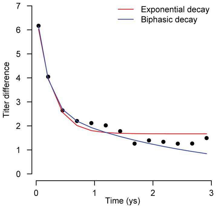
Biphasic and exponential decay curves fitted to HI antibody measurements following observed symptomatic infections.

Extended Data Figure 2. Variability in titer responses and measurement error and bias by serotype.

(A) Variability in titer responses. Violin plots showing median (black square), 25% and 75% quantiles (thick black line) and 95% distribution (in grey) of net titer rise at different time points following infection (N=1,420) (B) Estimated underlying differences across serotypes in the measurement of antibody levels by hemagglutination inhibition assay over and above that attributable to infection (DENV1 is reference) with 95% credible intervals (fitted to data from 140,612 titer measurements). (C) Mean estimated error in the hemagglutination inhibition assay estimated with 95% credible intervals using our model results (grey) and empirically derived (blue) from 795 repeated measurements on the same serum compared to that previously empirically derived estimated for plaque reduction neutralization tests (PRNTs) (blue).

Extended Data Figure 3. Serotype distributions.

(A) Distribution of serotypes by year comparing the detected symptomatic infections by PCR and the augmented primary infections where we could confidently assign the serotype (>50% of model iterations inferring the same serotype). We could confidently assign the serotype in 60% of instances. (B) Serotype distribution for detected symptomatic primary infections and augmented subclinical primary infections where the infecting serotype could be confidently assigned (>50% of model iterations inferring the same serotype). (C) Distribution of serotypes by year comparing the detected symptomatic infections by PCR and the augmented primary infections using a more stringent cutoff that >75% of model iterations infer the same serotype. In this scenario we could confidently assign the serotype in 32% of instances.

Extended Data Figure 4. Cox proportional hazards model versus logistic regression.

Comparison of results using time varying cox proportional hazards model (dashed line) with that from logistic regression (solid line) for the annualized probability of (A) infection, (B) developing any symptoms, (C) being hospitalized and (D) developing DHF as a function of the mean measured antibody titer across all serotypes at the time of exposure using titer data from all study subjects (N-3,451). The open circles on the left represent primary infections (i.e., those with no detectable titers to any serotype prior to exposure). The shaded regions represent 95% bootstrap confidence intervals. To calculate probabilities, the relative hazards from the cox model are multiplied by the baseline hazard for those with measured titers of 0 (calculated as proportion of person-time with an infection time among those with measured titers of 0).

Extended Data Figure 5. Receiver Operating Characteristic to identify DHF infections.

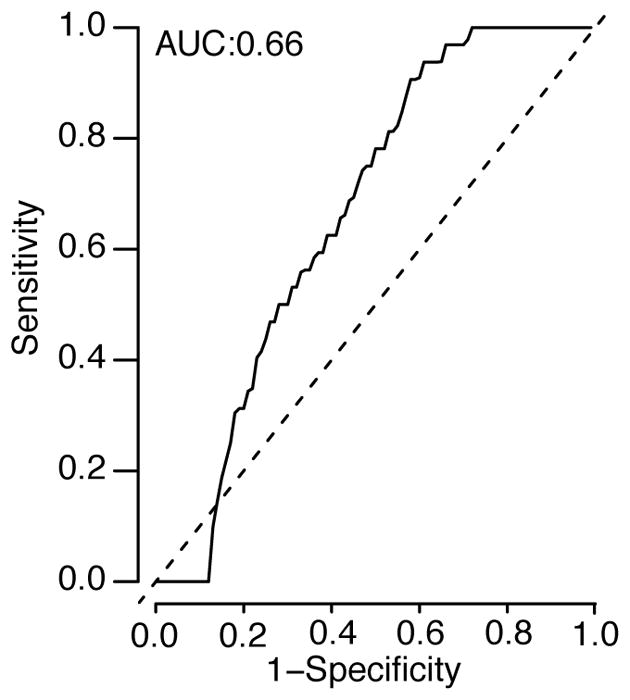
Ability of modelled relationship between measured HI titer and risk of DHF to identify those with DHF using those with DHF compared to randomly selected matched controls from individuals in the cohort who had detectable titers at the same time (N=36 with DHF with the same number of matched controls).

Extended Data Figure 6. Probability of disease as a function of HI and PRNT titer.

Probability of disease as a function of mean titer across the four types at the time of infection. (A) For those infected during the surveillance windows, the probability of developing any symptoms as a function of mean titer (N=781). (B) For those infected during the surveillance windows, the probability of being hospitalized (N=781). (C) For those infected during the surveillance windows, the probability of developing DHF as a function of mean titer (N=781). (D) For those infected during the surveillance windows (N=781), the probability of developing any symptoms as a function of mean PRNT titer. (E) For those infected, the probability of being hospitalized as a function of mean PRNT titer. (F) For those infected, the probability of developing DHF as a function of mean PRNT titer. In each panel, the open circles on the left represent primary infections. The shaded region represents 95% confidence intervals.

Extended Data Figure 7. Population-level distribution of titers by birth cohort and age.

(A) Proportion of cohort who are naïve as a function of time. (B) Proportion of cohort who are naïve as a function of age. Proportion of cohort with titers above risk zone (i.e., greater than 3) as a function of time (C) and age (D).

Extended Data Figure 8. Receiver Operating Characteristic for infection detection under different testing protocols.

The ROC for different assay approaches and time between blood draws calculated from 100,000 simulated titer responses. (A) Single serotype assay – if HIs are conducted for just a single serotype at two time points. (B) HIs conducted against all four serotypes. Infections are considered to occur if the ratio of any of the four titers at time point 2 versus time point 1 is greater than the threshold value. (C) HIs conducted against all four serotypes. Infections are considered to occur if the ratio of the mean of the four titers at time point 2 versus the mean at time point 1 is greater than the threshold value.

Extended Data Figure 9. Performance of assay dependent on time between blood draws and measurement error.

Optimization of assays in detection of events where specificity is maintained at >95%. We explore the performance of three different assay testing protocols: current practice where infection events are defined as a rise above a cut-point in any serotype across two blood draws (A), ‘mean approach’ where the mean across all serotypes is first calculated before comparing across time points (B), ‘mean approach’ where titers are available on a continuous scale (C). For each protocol, we identify the optimal cut-point for a range of assay measurement errors from 100,000 simulated titers based on the fitted titer responses from infections in our study population, that maintains a specificity of >95% (top row). We then calculate the sensitivity of the approach for different time intervals between blood draws using 50% held out data (bottom row). (D)–(F) Same as (A)–(C) but using a more stringent 99% cut-off.

Extended Data Figure 10. Clustering of symptomatic (N=274) and subclinical cases (mean N=507 across 100 reconstructed datasets) by school by time and serotype.

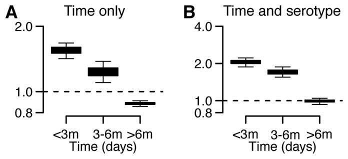
(A) Probability of observing an augmented subclinical infection (irrespective of serotype) occurs at different time intervals within the same school of a detected symptomatic case relative to the probability of observing an augmented subclinical infection occurring in a different school in that same time interval. (B) For augmented primary infections that are consistently of the same serotype (defined as >50% of augmented datasets have a primary infection in the same individual caused by the same serotype in the same six-month time window). Probability that an augmented primary infection that occurs within a fixed time window of a PCR-confirmed case and in the same is of the same serotype relative to the probability that an augmented primary infection that occurs within the same time window in a different school is of the same serotype. Note that the modelling framework can only allow differentiation of serotypes for primary infections. Cross-reaction prevents differentiation in post-primary infections. Overall, 60% of primary infections have a consistent serotype for a primary infection across augmented datasets. Each boxplot presents the 2.5%, 25%, 75% and the 97.5% quantiles of the distribution as well as the mean.

References

- 1.Undurraga EA, Halasa YA, Shepard DS. Use of expansion factors to estimate the burden of dengue in Southeast Asia: a systematic analysis. PLoS Negl Trop Dis. 2013;7:e2056. doi: 10.1371/journal.pntd.0002056. [DOI] [PMC free article] [PubMed] [Google Scholar]
- 2.Endy TP, et al. Epidemiology of inapparent and symptomatic acute dengue virus infection: a prospective study of primary school children in Kamphaeng Phet, Thailand. American Journal of Epidemiology. 2002;156:40–51. doi: 10.1093/aje/kwf005. [DOI] [PubMed] [Google Scholar]
- 3.Cauchemez S, Ferguson NM. Methods to infer transmission risk factors in complex outbreak data. J R Soc Interface. 2012;9:456–469. doi: 10.1098/rsif.2011.0379. [DOI] [PMC free article] [PubMed] [Google Scholar]
- 4.Bhatt S, et al. The global distribution and burden of dengue. Nature. 2013;496:504–507. doi: 10.1038/nature12060. [DOI] [PMC free article] [PubMed] [Google Scholar]
- 5.Halstead SB. Dengue. Imperial College Press; London: 2008. [Google Scholar]
- 6.Vaughn DW, et al. Dengue in the early febrile phase: viremia and antibody responses. J Infect Dis. 1997;176:322–330. doi: 10.1086/514048. [DOI] [PubMed] [Google Scholar]
- 7.Harris E, et al. Clinical, epidemiologic, and virologic features of dengue in the 1998 epidemic in Nicaragua. The American Journal of Tropical Medicine and Hygiene. 2000;63:5–11. doi: 10.4269/ajtmh.2000.63.5. [DOI] [PubMed] [Google Scholar]
- 8.Venturi G, et al. Humoral immunity and correlation between ELISA, hemagglutination inhibition, and neutralization tests after vaccination against tick-borne encephalitis virus in children. J Virol Methods. 2006;134:136–139. doi: 10.1016/j.jviromet.2005.12.010. [DOI] [PubMed] [Google Scholar]
- 9.Katzelnick LC, et al. Antibody-dependent enhancement of severe dengue disease in humans. Science. 2017;358:929–932. doi: 10.1126/science.aan6836. [DOI] [PMC free article] [PubMed] [Google Scholar]
- 10.Halstead SB, Rojanasuphot S, Sangkawibha N. Original antigenic sin in dengue. The American Journal of Tropical Medicine and Hygiene. 1983;32:154–156. doi: 10.4269/ajtmh.1983.32.154. [DOI] [PubMed] [Google Scholar]
- 11.Clapham HE, et al. Dengue Virus (DENV) Neutralizing Antibody Kinetics in Children After Symptomatic Primary and Postprimary DENV Infection. J Infect Dis. 2016;213:1428–1435. doi: 10.1093/infdis/jiv759. [DOI] [PMC free article] [PubMed] [Google Scholar]
- 12.Salje H, et al. Variability in dengue titer estimates from plaque reduction neutralization tests poses a challenge to epidemiological studies and vaccine development. PLoS Negl Trop Dis. 2014;8:e2952. doi: 10.1371/journal.pntd.0002952. [DOI] [PMC free article] [PubMed] [Google Scholar]
- 13.Salje H, et al. Dengue diversity across spatial and temporal scales: local structure and the impact of host population size. Science. 2017 doi: 10.1126/science.aaj9384. [DOI] [PMC free article] [PubMed] [Google Scholar]
- 14.Rodriguez-Barraquer I, et al. Revisiting rayong: shifting seroprofiles of dengue in Thailand and their implications for transmission and control. American Journal of Epidemiology. 2014;179:353–360. doi: 10.1093/aje/kwt256. [DOI] [PMC free article] [PubMed] [Google Scholar]
- 15.Serotype-specific differences in the risk of dengue hemorrhagic fever: an analysis of data collected in Bangkok, Thailand from 1994 to 2006. 2010;4:e617. doi: 10.1371/journal.pntd.0000617. [DOI] [PMC free article] [PubMed] [Google Scholar]
- 16.Duong V, et al. Asymptomatic humans transmit dengue virus to mosquitoes. Proc Natl Acad Sci USA. 2015;112:14688–14693. doi: 10.1073/pnas.1508114112. [DOI] [PMC free article] [PubMed] [Google Scholar]
- 17.D’Agostino RB, et al. Relation of pooled logistic regression to time dependent Cox regression analysis: the Framingham Heart Study. Stat Med. 1990;9:1501–1515. doi: 10.1002/sim.4780091214. [DOI] [PubMed] [Google Scholar]
- 18.Ferguson NM, et al. Benefits and risks of the Sanofi-Pasteur dengue vaccine: Modeling optimal deployment. Science. 2016;353:1033–1036. doi: 10.1126/science.aaf9590. [DOI] [PMC free article] [PubMed] [Google Scholar]
- 19.Kliks SC, Nimmanitya S, Nisalak A, Burke DS. Evidence that maternal dengue antibodies are important in the development of dengue hemorrhagic fever in infants. The American Journal of Tropical Medicine and Hygiene. 1988;38:411–419. doi: 10.4269/ajtmh.1988.38.411. [DOI] [PubMed] [Google Scholar]
- 20.Guzmán MG, Alvarez M, Halstead SB. Secondary infection as a risk factor for dengue hemorrhagic fever/dengue shock syndrome: an historical perspective and role of antibody-dependent enhancement of infection. Arch Virol. 2013;158:1445–1459. doi: 10.1007/s00705-013-1645-3. [DOI] [PubMed] [Google Scholar]
- 21.Villar L, et al. Efficacy of a tetravalent dengue vaccine in children in Latin America. N Engl J Med. 2015;372:113–123. doi: 10.1056/NEJMoa1411037. [DOI] [PubMed] [Google Scholar]
- 22.Moodie Z, et al. Neutralizing Antibody Correlates Analysis of Tetravalent Dengue Vaccine Efficacy Trials in Asia and Latin America. J Infect Dis. 2018;217:742–753. doi: 10.1093/infdis/jix609. [DOI] [PMC free article] [PubMed] [Google Scholar]
- 23.Cummings DAT, Schwartz IB, Billings L, Shaw LB, Burke DS. Dynamic effects of antibody-dependent enhancement on the fitness of viruses. Proc Natl Acad Sci USA. 2005;102:15259–15264. doi: 10.1073/pnas.0507320102. [DOI] [PMC free article] [PubMed] [Google Scholar]
- 24.Wearing HJ, Rohani P. Ecological and immunological determinants of dengue epidemics. Proc Natl Acad Sci USA. 2006;103:11802–11807. doi: 10.1073/pnas.0602960103. [DOI] [PMC free article] [PubMed] [Google Scholar]
- 25.Flasche S, et al. The Long-Term Safety, Public Health Impact, and Cost-Effectiveness of Routine Vaccination with a Recombinant, Live-Attenuated Dengue Vaccine (Dengvaxia): A Model Comparison Study. PLoS Med. 2016;13:e1002181. doi: 10.1371/journal.pmed.1002181. [DOI] [PMC free article] [PubMed] [Google Scholar]
- 26.Adams B, et al. Cross-protective immunity can account for the alternating epidemic pattern of dengue virus serotypes circulating in Bangkok. Proc Natl Acad Sci USA. 2006;103:14234–14239. doi: 10.1073/pnas.0602768103. [DOI] [PMC free article] [PubMed] [Google Scholar]
- 27.Grenfell BT, Bjørnstad ON, Kappey J. Travelling waves and spatial hierarchies in measles epidemics. Nature. 2001;414:716–723. doi: 10.1038/414716a. [DOI] [PubMed] [Google Scholar]
- 28.Earn DJ, Rohani P, Bolker BM, Grenfell BT. A simple model for complex dynamical transitions in epidemics. Science. 2000;287:667–670. doi: 10.1126/science.287.5453.667. [DOI] [PubMed] [Google Scholar]
- 29.Cobey S, Lipsitch M. Niche and neutral effects of acquired immunity permit coexistence of pneumococcal serotypes. Science. 2012;335:1376–1380. doi: 10.1126/science.1215947. [DOI] [PMC free article] [PubMed] [Google Scholar]
- 30.Mammen MP, et al. Spatial and temporal clustering of dengue virus transmission in Thai villages. PLoS Med. 2008;5:e205–e205. doi: 10.1371/journal.pmed.0050205. [DOI] [PMC free article] [PubMed] [Google Scholar]
- 31.Salje H, et al. Revealing the microscale spatial signature of dengue transmission and immunity in an urban population. Proc Natl Acad Sci USA. 2012;109:9535–9538. doi: 10.1073/pnas.1120621109. [DOI] [PMC free article] [PubMed] [Google Scholar]
- 32.Endy TP. Spatial and Temporal Circulation of Dengue Virus Serotypes: A Prospective Study of Primary School Children in Kamphaeng Phet, Thailand. American Journal of Epidemiology. 2002;156:52–59. doi: 10.1093/aje/kwf006. [DOI] [PubMed] [Google Scholar]
- 33.Smith T, Vounatsou P. Estimation of infection and recovery rates for highly polymorphic parasites when detectability is imperfect, using hidden Markov models. Stat Med. 2003;22:1709–1724. doi: 10.1002/sim.1274. [DOI] [PubMed] [Google Scholar]
- 34.Reich NG, et al. Interactions between serotypes of dengue highlight epidemiological impact of cross-immunity. J R Soc Interface. 2013;10:20130414–20130414. doi: 10.1098/rsif.2013.0414. [DOI] [PMC free article] [PubMed] [Google Scholar]
- 35.Rudolph KE, Lessler J, Moloney RM, Kmush B, Cummings DAT. Incubation periods of mosquito-borne viral infections: a systematic review. J Trop Med Hyg. 2014;90:882–891. doi: 10.4269/ajtmh.13-0403. [DOI] [PMC free article] [PubMed] [Google Scholar]
- 36.White MT, et al. A combined analysis of immunogenicity, antibody kinetics and vaccine efficacy from phase 2 trials of the RTS,S malaria vaccine. BMC Med. 2014;12:117. doi: 10.1186/s12916-014-0117-2. [DOI] [PMC free article] [PubMed] [Google Scholar]
- 37.Therneau T, Crowson C, Atkinson E. Using time dependent covariates and time dependent coefficients in the cox model. Survival Vignettes. 2017 [Google Scholar]
- 38.Lessler J, Salje H, Grabowski MK, Cummings DAT. Measuring Spatial Dependence for Infectious Disease Epidemiology. PLoS ONE. 2015;11:e0155249–e0155249. doi: 10.1371/journal.pone.0155249. [DOI] [PMC free article] [PubMed] [Google Scholar]
Associated Data
This section collects any data citations, data availability statements, or supplementary materials included in this article.