Improved Search of Large Transcriptomic Sequencing Databases Using Split Sequence Bloom Trees

Abstract

Enormous databases of short-read RNA-seq experiments such as the NIH Sequencing Read Archive are now available. These databases could answer many questions about condition-specific expression or population variation, and this resource is only going to grow over time. However, these collections remain difficult to use due to the inability to search for a particular expressed sequence. Although some progress has been made on this problem, it is still not feasible to search collections of hundreds of terabytes of short-read sequencing experiments. We introduce an indexing scheme called split sequence bloom trees (SSBTs) to support sequence-based querying of terabyte scale collections of thousands of short-read sequencing experiments. SSBT is an improvement over the sequence bloom tree (SBT) data structure for the same task. We apply SSBTs to the problem of finding conditions under which query transcripts are expressed. Our experiments are conducted on a set of 2652 publicly available RNA-seq experiments for the breast, blood, and brain tissues. We demonstrate that this SSBT index can be queried for a 1000 nt sequence in <4 minutes using a single thread and can be stored in just 39 GB, a fivefold improvement in search and storage costs compared with SBT.

1. Introduction

An enormous amount of DNA and RNA short read sequence data has been published worldwide. The NIH Sequence Read Archive (SRA) (Leinonen et al., 2011) alone contains almost six petabases of open-access sequence and continues to grow at an accelerating rate. This collection could be a great resource for understanding genetic variation, and condition- and disease-specific gene function in ways the original depositors of the data did not anticipate. For example, a natural use would be to search all public, human RNA-seq short-read files in the SRA (representing individual sequencing runs) for the presence of a particular transcript of interest to understand where and when it is expressed or to select a manageable subset of experiments for further analysis. However, searching the entirety of such a database for a query sequence has not been possible in reasonable computational time.

Some progress has been made toward enabling sequence search on large databases. The NIH SRA does provide a sequence search functionality (Camacho et al., 2009); however, it requires the selection of a small number of experiments to which to restrict the search. Existing full-text indexing data structures such as Burrows–Wheeler transform (Burrows and Wheeler, 1994), FM-index (Ferragina and Manzini, 2005), or others (Grossi and Vitter, 2005; Navarro and Mäkinen, 2007; Grossi et al., 2011) cannot at present be efficiently built at this scale. Word-based indices (Navarro et al., 2000; Ziviani et al., 2000), such as those used by Internet search engines, are not appropriate for edit distance-based biological sequence search. The sequence-specific solutions caBLAST and its variants (Loh et al., 2012; Daniels et al., 2013; Yu et al., 2015) require an index of known genomes, genes, or proteins, and so cannot search for novel sequences in unassembled read sets. Furthermore, all of these existing approaches do not handle the additional complication that a match to a query sequence q may span many short reads.

More recently, two methods have been developed that store the kmer content of a set of experiments in a directly searchable index. The sequence bloom tree (SBT) (Solomon and Kingsford, 2016) encodes an approximation of each experiment's kmer content in a single bloom filter and builds a directly searchable binary tree of bloom filters over increasingly large subsets of the data. Queries are processed by looking up each kmer in a query for their presence or absence in the tree and recursing until all matching leaves have been found. It represents the current best method for searching a large database but cannot handle petabase scale data. The bloom filter trie (BFT) (Holley et al., 2016) was designed as a direct compression method for a pan-genome and provides an exact index of kmer content that can be queried.

We address the search problem of finding all the experiments that contain enough reads matching a given query sequence to indicate that it was present in the experiment. A query is an arbitrary sequence such as a transcript, and we find the collection of short-read experiments in which that sequence is present. These estimates themselves could be used to analyze conditions of gene expression or could make downstream analysis more efficient by filtering a large database for the relevant files. The SBT was the first data structure to directly address this problem and could search a 5 terabase data set in <20 minutes using a 200 GB index. We modify the base structure of SBT with a new indexing data structure called split sequence bloom tree (SSBT). SSBT “splits” the bloom filters present in an SBT into two distinct filters that store unique subsets of the base filter as described in Section 2.1. In addition to this novel storage strategy, the SSBT method introduces the concept of a “noninformative bit” (Section 2.3) and uses a more efficient query algorithm that can prune query indices when universal matches or mismatches are found in a subtree (Section 2.5). These novel elements are the basis of the space and time improvements described hereunder.

SSBT also extends a number of important properties found in SBT. Like SBT, SSBT is independent of the eventual queries, so the approach is not limited to searching only for known genes, but can potentially identify arbitrary sequences. SSBTs can be efficiently built, extended, and stored in limited space and do not require retaining the original sequence files to process queries. Using SSBTs, data sets can be searched using low memory for the existence of arbitrary query sequences. We compared SSBT against BFT and SBT and found that it outperforms in terms of both query time (5 times faster than SBT and 15 times faster than BFT) and storage cost, at the price of some additional time and temporary storage needed to construct the index.

2. Methods

2.1. Split sequence bloom tree

The main idea behind SSBT is the creation of a hierarchy of compressed bloom filters (Bloom, 1970; Broder and Mitzenmacher, 2005), which is used to efficiently store a set of experiments, each consisting of many short reads (Fig. 1). A bloom filter is a probabilistic storage structure that encodes an arbitrary set into a fixed length bit vector using hash functions. As in the SBT, each bloom filter here encodes the set of k-mers (length—k subsequences) present within a subset of the sequencing experiments and is stored using hash functions that convert these kmers to a specific index on the filter. We denote the kmer content of each experiment i by the set b_i, with the collection 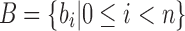denoting a set of n experiments represented by their kmer content. Throughout, we abuse notation slightly to identify bloom filters with the sets they represent.

FIG. 1.

Example uncompressed and compressed SSBT. Black corresponds to a bit value of “1” and white corresponds to a bit value of “0.” (a) Gray bits correspond to noninformative bits whose value is known (always 0) given a parent filter. We see that gray bits are cumulative and exist at all index positions below a “1” in the sim filter or a “0” in the rem filter. When looking up index value 5, each filter is queried until either a sim “1” is found or a rem “0” is found. This search is represented by the blue outlined square. (b) All noninformative bits have been removed from the uncompressed tree (RRR does not change the bit values and is not represented in the figure). The lookup for index value 5 is adjusted based on the removed noninformative bits. SSBT, split sequence bloom tree.

An SSBT is a binary tree that stores each b_i in B across a unique path from root to leaf with each leaf mapping to a single experiment. This is a change from the SBT, which stores each b_i in B both as a unique leaf and in each node from root to leaf. The root node r of an SSBT contains the total content of each b_i and stores this information using two identically sized bloom filters using the same hash function; we define the pair of bloom filters at a node as a single “split bloom filter.” The first filter, the similarity filter, stores the universally expressed kmers in set B. The second filter, the remainder filter, stores the remaining kmers—those kmers in B that are not universally expressed but exist in at least one experiment.

More specifically, for a given node r containing n experiments in its subtree, we define the similarity filter, , as the intersection of all b_i in B. We define the remainder filter, , as the bloom filter that stores the remaining kmers—those in the union of all b_i excluding those found in the similarity vector. By this definition, the bitwise union of and is equivalent to a single bloom filter that stores all b_i in B. Furthermore, the bitwise intersection of and is the empty set. Different kmers in B may hash to the same position in . Because of this, additional “similarity” may be found by random chance when hashing kmers. The inverse (identical kmers mapping to different positions) is not possible in a bloom filter.

Given the root r, only the kmers that are stored in are then passed to the children. In this way r's immediate children do not store the full set b_i but rather the modified . This sparsification continues from root to leaf with 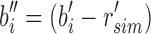and more generally takes the form of a recurrence relationship 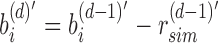for the depth d node on an arbitrary path from root to leaf. A leaf at depth d stores in its sim filter. The leaf's rem filter is defined as , which is the empty set. We can recover the original set of kmers for each experiment by following the unique path from root to leaf and computing .

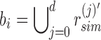2.2. Split sequence bloom tree construction and insertion

An SSBT inherits the same general build process as an SBT and is built by repeated insertion of sequencing experiments followed by the removal of all so-called noninformative bits from each filter. We first describe the process to insert an experiment; Section 2.3 defines noninformative bits. Given an (possibly empty) SSBT T, a new sequencing experiment s can be inserted into T by first computing the fixed-length bloom filter b_s of the kmers present in s and then walking from the root along a path to the leaves and inserting s at the bottom of T in the following way. When at node u, if u has children, b_s has to be split between and . This is done through the bit updates defined in Table 1 for each bit index i in . These updates ensure that u correctly stores what is still universally similar in and what now exists below u in the tree with and that b_s has been updated to store similar elements at u.

Table 1.

Bit Update Table When Inserting into the Subtree Rooted at u

	Before			After
(i)	1	0	1	—	—	0	—
(ii)	1	0	0	0	1	—	1
(iii)	0	1	1	—	—	—	—
(iv)	0	1	0	—	—	—	—
(v)	0	0	1	—	1	—	—
(vi)	0	0	0	—	—	—	—

u's two immediate children are both updated with the single column . A value of “—” implies that no change needs to be made to that bit. (i) contains a value already stored in , the value is removed from . (ii) does not contain a value stored in . Although the bit is no longer similar at u, has not yet been inserted into a child and all current children of u are universally similar at this location. (v) contains a value not found in the tree. is updated to reflect that the value now exists. (iii, iv, vi) No changes need to be made.

The potentially modified b_s is then compared against each child c of u to find the “most similar” child. This greedy insertion strategy attempts to maximize the similarity in a branch to produce the smallest SSBT with the most efficient branch pruning. Although we tested many similarity metrics for comparing a single filter with a split filter , the metric used in the experiments reported hereunder chooses the child with the largest number of shared 1-bits between and b_s. If no child has any 1-bits in common with b_s, the metric then selects the child with the smallest Hamming distance between b_s and . The most similar child then becomes the new current node, and the process is repeated with a new subtree. If u has no children, then u represents a sequencing experiment and only contains one vector . In this case, a new node v is created as a child of u's parent with u and b_s as v's children. As both and b_s are leaves, is the bit intersection of u and b_s, whereas is the bit union of and . Finally, we remove the elements in this new parent node from both children by replacing u with and b_s with . This yields an uncompressed SSBT containing all previous nodes and two new nodes v and b_s.

2.3. Noninformative bits in split sequence bloom tree

Given the definition of SSBT's split filters already described, for an arbitrary node u the only values allowed at a particular index i are . However, every index is represented using a bit from either filter, even when one filter's value clearly defines the other. We address this inefficiency by removing these “noninformative bits” from the tree. We define a noninformative bit as a bit index i present in node u whose value can be determined by examining the bloom filters present in the set of parent filters above u. We describe the cases of noninformativity in SSBT hereunder and provide an example in Figure 1:

• (1)For a bit index i, if , then for every descendant c of u, and i is noninformative below u. This is a direct result of the definition of as the union of all children below it.
• (2)For a bit index i, if then and is noninformative. This is a result of the fact that the rem filter only contains the elements thaat are not stored in the sim filter.
• (3)For a bit index i, if then for every descendent c of u, and i is noninformative below u. This is a consequence of applying (1) to (2).

Using these cases, we can remove all noninformative bits from given , and we can remove all noninformative bits from u's immediate children using both and . As bits are only ever removed, for a node u and its child c, . These removed bits lead to size reductions for all subsequent filters. SSBTs are most efficient when there is a large amount of uniformity in the experiments being stored at u in terms of either uniform expression of kmers or uniform absence of any kmer hashing to a particular bit.

2.4. Split sequence bloom tree compression

Given an uncompressed SSBT T with bloom filters of fixed length m and conserved hash function, we build a compressed SSBT by removing all noninformative bits (defined in Section 2.3) from T and compressing the variable length filters using Raman-Raman-Rao (RRR) compression (Raman et al., 2002). After removing noninformative bits from vector u, we obtain a smaller vector . The total number of informative bits in and , as well as their indices, can be determined using two filters: u's immediate parent's rem filter, , and . We define to be the number of bits set to x in the bit vector u from index . We compute this value in time for a vector of size by storing extra bits as described as part of the 64-bit rank9 function (Vigna, 2008) and implemented in the C++ package sdsl (Gog et al., 2014). For vectors of size bits or less, this can be considered a near-constant time method.

Given , the only informative bits in are those i for which and . Likewise given , the only informative bits in are those i in which both and and . At each i, the values in and determine whether i is informative. If i is informative, it is appended to the next position in and/or . Subsequently, is compressed through the RRR (Raman et al., 2002) compression scheme, which allows querying a bit without decompression and incurs only an factor increase in access time (where m is the size of the bloom filter with noninformative bits removed). This process operates for every node in the tree, starting with the root node T that has a full length because it has no parent. See Figure 1 for an example of the compression step.

2.5. Split sequence bloom tree querying

Given a query sequence q and a compressed SSBT T, the sequencing experiments that contain q can be found by breaking q into its constituent set of kmers K_q and then flowing these kmers over T starting from the root. In an SSBT, these kmers are organized into a set of unique kmers and immediately converted into a vector of filter indices using the hash functions defined by T's root's sim filter. At the root node u, we query first for each index in V_q. Matches in are recorded as “universal hits” since they are found in intersection of all experiments rooted beneath u. The count of all universal hits represents a lower bound on the number of matching kmers in all experiments rooted below u. Indices that are universal hits do not have to be queried further and are removed from the set—the sum of these hits records their presence at all children of u. The remaining indices that were not found in are then queried in . As , this query is accomplished by adjusting all indices V_i V_q to account for the noninformative bits that were removed. As we have already converted kmers to hash values, we transition from to by subtracting the number of 1-bits that occurred before V_i in . This is simply the , a property of a bit vector that can be computed in constant time using RRR-compressed vectors.

Each modified index can then be queried in . Indices that map to 0-bits do not have to be queried further as they do not exist in any child to u. Indices that map to 1-bits are potential hits that belong to at least one child below u but not all. By adding the number of potential hits in with the number of universal hits found in , an upper bound on the number of matching kmers is determined for each query. If, for a user-specified cutoff , this count is less than , then the query cannot exist in this subtree and the subtree is not searched further (it is pruned). If there exist or more universal matches, every child beneath u is a query hit and the tree also does not have to be searched further. Only in the case where the count is greater than but not enough universal matches have been found do we have to proceed to u's children. To transition each index from node u to child node c, each index has to be further adjusted by the number of 0-bits in . Once again, this can be calculated in constant time using . By repeating this process down through the tree, SSBT efficiently prunes branches that cannot contain the query, prunes queries that are known to exist in all children, and maintains a consistent hash function across a variable length set of compressed filters. After searching or pruning every branch, the set of leaves that contain the query are then returned. An example of this query process can be found in Figure 1.

Using this process, not all query indices are searched at each node in the tree. All indices are initially searched in an “active” state but may be pruned to “inactive” if a universal match or mismatch is found. To prevent having to store a unique query set for every node in the tree, we stored V_q only once outside of the SSBT structure and developed a reversible means of activating or deactivating an index, as well as reversing changes made to the index value when descending the tree. Given a vector of indices V_q, we define a single integer—the tail-index—to be the position along the V_q vector that contains the last “active” query index. This tail-index is initialized to the final value in V_q and queries that are “deactivated” simply swap positions with the tail-index, and the tail-index is decremented by 1. In such a way, we store the full set of indices but only query those indices up to and including the tail-index. By storing the tail-index present in each node (a cost of a single integer per node), we can restore all queries that were active at that node. Because the tail-index defines both the pivot between “active” and “inactive” and the swap position for deactivating an index, the order in the vector records the order of deactivation. Because of this, any index that was “active” for an arbitrary node u with tail-index k will always be among the first k indices in V_q and can be reactivated as the tree traversal pops back up the tree. Thus using the tail-index, we can exactly store the unique set of indices that need to be searched at any node using only a single vector and an integer at each node.

“Active” indices in V_q also have their values adjusted at each step to match the change in size between and and between u and u's children. Given an index position that maps to , we can reconstruct the index position that maps to by looking up the -th informative bit in . As defines noninformativity, we simply find the -th 0 in . This can be done using the operation, which is defined to be the index position of the j-th bit set to x in the bit vector u. For an RRR-compressed vector, can be computed in time for a length m vector. Likewise, given an index position mapping to an arbitrary child node of u, , we can recover the index position mapping to by finding the -th informative bit in . As defines noninformativity, we simply find the -th 1 in . For an RRR-compressed vector, this can be computed in time for a length m vector using the operation. Thus, using just the rank and select operations implicit to an RRR-compressed vector, we can recover any index position at any node given a position along the SSBT and the SSBT split bloom filters themselves.

2.6. Accuracy

SSBT builds off of the base bloom filters used in SBT and encodes the same information found in the leaves of an SBT. The innovations introduced here improve upon the efficiency of that encoding and provide additional information to facilitate rapid search but an SSBT will always yield an identical set of results as SBT. As it has been shown that kmer similarity is highly correlated to the quality of the alignments between sequences (Rasmussen et al., 2006; Philippe et al., 2013; Zhang et al., 2014; Brown et al., 2015), and SBT has previously determined the accuracy of this metric (Solomon and Kingsford, 2016), we did not investigate the accuracy of SSBT, which is the same as SBT, further here. One can think of SSBT as a lossless compression and reorganization scheme on SBTs that operates before RRR-compression.

3. Results

3.1. Data and hardware

We used a set of 2652 human, RNA-seq short-read runs from the NIH SRA (Leinonen et al., 2011). At the time of download, these files consisted of the entire set of publicly available, human RNA-seq runs from blood, brain, and breast tissues stored at the SRA (as determined by keywords in their metadata and excluding files sequenced using the SOLiD technology). This data set has a total size of 5 TB of raw SRA data or 2.7 TB of gzipped fasta sequences. The 50 files for the comparison with BFT were chosen at random from this set and have a total size of 49 GB of gzipped fasta sequences. Kmer counts were computed using the Jellyfish 2.0 library for SBT and SSBT and KMC 2.0 for BFT. Jellyfish counts were constructed using the SBT “count” command using an expected kmer set size of and a single hash function. All times in these experiments were obtained on a shared computer with 16 Intel Xeon 2.60 GHz cores using a single thread. BFT was run using default options with a compression constant of 50. SBT and SSBT use a kmer size of 20, whereas BFT was built using a kmer size of 18 as it only allows kmer lengths that are multiples of 9.

3.2. Evaluation on build time and storage cost

We compared the construction costs associated between SBT version 0.3.5, SSBT version 0.1, and BFT version 0.8.1 by measuring their respective build time, maximum memory cost during construction, and storage cost of the resulting 100 experiment index. SBT and SSBT's RAM loads are controlled by setting the maximum number of filters allowed to be loaded simultaneously. We manually adjusted these values to be roughly equivalent to BFT by setting SBT's maximum in-memory filter load to 100 nodes, with a measured peak RAM of 24.2 GB, and SSBT was limited to 30 in-memory nodes, with a measured peak RAM of 16.2 GB. This is in line with our expectations that an uncompressed SSBT internal node is roughly twice as large as an SBT node and requires a more complicated build process. In addition, as BFT uses a different kmer counting tool (KMC2 vs. Jellyfish), the build time records only the time required to construct an index from a precomputed set of kmer counts. These results, which are summarized in Tables 2 and 3, indicate that BFT takes 11 times longer to build than the combined time to build and compress an SBT and yields an index over three times larger. Similarly SSBT builds and compresses 3.8 times faster than BFT and yields a directly searchable index with less than 1/13th the total storage cost. We note that this is not a strictly apples-to-apples comparison as BFT exactly encodes the kmer set for each experiment, whereas SBT and SSBT are approximate indices with a high false positive for any one kmer.

Table 2.

Build and Compression Peak RAM Loads and On-disk Storage Costs for Sequence Bloom Tree, Split Sequence Bloom Tree, and Bloom Filter Trie Constructed from a 50 Experiment Set

Data index	BFT	SBT	SSBT
Build peak RAM (GB)	21.2	21.5	15.6
Compress peak RAM (GB)	—	24.2	16.2
Uncompressed size (GB)	—	24	35
Compressed size (GB)	13	3.9	0.94

As BFT's built-in compression tool is a core part of its build process, we report only a single value for RAM and final size for BFT.

BFT, bloom filter trie; SBT, sequence bloom tree; SSBT, split sequence bloom tree.

Table 3.

Build and Compression Times for Sequence Bloom Tree, Split Sequence Bloom Tree, and Bloom Filter Trie Constructed from a 50 Experiment Set

Data index	BFT	SBT	SSBT
Build time (minutes)	137	6	19
Compression time (minutes)	—	6.5	17
Total time (minutes)	137	12.5	36

As SBT and SSBT were designed to be queried from a compressed state, we compare the time to build and compress against BFT's time to build.

We also performed a large scale analysis between SBT and SSBT using the full 2652 experiment set. Both SBT and SSBT were run with a maximum of 100 tree nodes in memory, with a peak memory of roughly 24 and 48 GB, respectively. The results from this analysis are summarized in Table 4 and show that SSBT is still roughly three times slower to build and compress than the SBT. We note that the large scale SSBT is much less efficient to build, whereas much more efficient to compress than the small scale test.

Table 4.

Build Statistics for Sequence Bloom Tree and Split Sequence Bloom Tree Constructed from a 2652 Experiment Set

Data index	SBT	Split SBT
Build time (hours)	18	78
Compression time (hours)	17	19
Uncompressed size (GB)	1295	1853
Compressed size (GB)	200	39.7

The sizes are the total disk space required to store a bloom tree before or after compression. In SSBT's case, this compression includes the removal of noninformative bits.

The bold values represent the on-disk storage cost for a complete, searchable tree.

We hypothesize that the more complex construction scheme, as well as the storage costs associated with storing two bloom filters in each internal node, scales poorly with database size and negatively impacts the build time. Meanwhile, the improvements in compression time are primarily a consequence of the noninformative bits. Specifically, as these noninformative bits do not need to be compressed and are cumulative, it becomes increasingly efficient to compress filters as one descends the tree. This has a much more significant effect at large scales wherein the accumulation of noninformative bits at low depths affects a greater number of nodes. In addition, we predict that there should be more noninformative bits overall given a larger population of experiments organized to maximize similarity in each subtree. This is supported by the fact that the average size of a compressed leaf filter is smaller in the large scale SSBT than the small scale SSBT, implying that more bits were removed on average from each individual experiment.

Although the ratio of build times remained roughly the same, the SSBT is demonstrably more efficient to store at large scales, yielding a fivefold reduction in overall size. As the indices only need to be built once (and can be incrementally built from the uncompressed state), the SSBT is a superior choice when there is sufficient hardware support for its larger uncompressed size. We further note that even this size (1853 GB) is significantly smaller than the raw data, that this size includes the bloom filter representation of every experiment, and that the raw data are not needed during the search once the bloom filter is constructed.

3.3. Evaluation of the query time

We evaluated the efficiency of queries in SBT, SSBT, and BFT on three sets of 100 queries. To build each query set, we estimated the expression profiles of all 50 experiments used in the small scale indices using Sailfish (Patro et al., 2014). We then randomly sampled transcripts that were expressed at transcripts per million (TPM) values at or more than 100, 500, or 1000 in at least one of those files to build three query sets of 100 queries each. Each query was run individually for each tool and the file system cache was emptied at the end of each run to ensure that the average time is an accurate representation of query behavior. The results are summarized in Table 5 and show that SSBT is anywhere from 3 × to 15 × faster than either method at this scale. Although this is a significant improvement, we suspect that this 50-experiment test underestimates SSBTs relative performance due to SSBTs efficient storage of similar elements and better optimized querying. We further note that this comparison is not strictly fair to BFT as it returns exact kmer content rather than approximate content. In practice, this would yield significantly fewer false positives, which may be preferred in certain contexts.

Table 5.

Comparison of Query Timing (and Average Peak Memory) Between Sequence Bloom Tree, Split Sequence Bloom Tree, and Bloom Filter Trie Indices for 50 Experiments

Index	TPM ≥100	TPM ≥500	TPM ≥1000
BFT	85 seconds (11.5 GB)	84 seconds (11.5 GB)	84 seconds (11.5 GB)
SBT	19 seconds (2.9 GB)	21 seconds (3.1 GB)	22 seconds (3.2 GB)
SSBT	5.8 seconds (0.64 GB)	6.2 seconds (0.65 GB)	6.3 seconds (0.66 GB)

TPM, transcripts per million.

A larger scale comparison was performed using the full 2652-experiment indices with SBT and SSBT. The query sets used in this analysis were randomly selected to exist in at least 1 of 100 randomly sampled experiments out of the full data set with three TPM-specific sets constructed as before. Each query was run individually and the results are summarized in Tables 6 and 7 and show that SSBT is more than five times faster than SBT regardless of the TPM value or cutoff threshold used in either index.

Table 6.

Comparison of Query Times Between Sequence Bloom Tree and Split Sequence Bloom Tree for 2652 Experiments

Index	TPM ≥100	TPM ≥500	TPM ≥1000
SBT (minutes)	19.7	20.7	20
SSBT (minutes)	3.7	3.8	3.6

Table 7.

Comparison of Query Times Using Different Thresholds for Sequence Bloom Tree and Split Sequence Bloom Tree Using Queries Found at TPM ≥ 100

Query time	= 0.7	= 0.8	= 0.9
SBT (minutes)	20	19	17
SSBT (minutes)	3.7	3.5	3.2
RAM SSBT (seconds)	31	29	26

“RAM SSBT” describes a hardware-accelerated search enabled locally based on the SSBT's smaller index size. A similar improvement in speed would be possible on SBT given the necessary hardware.

Given that SSBT's speed improvement closely mirrors its size improvement (a fivefold speedup for a fivefold size reduction), we hypothesized that SSBT could be made significantly faster by reducing or eliminating the I/O costs associated with loading and unloading bloom filters. Both SBT and SSBT are likely to benefit from this engineering adjustment, but under our hardware specifications, this is only possible for an SSBT, whose directly searchable index uses <1% of the size of the original data. This resulted in an additional 7 × speedup over regular SSBT and a roughly 39 × increase over SBT. We report this result as “RAM SSBT” in Table 7.

SSBT's speed improvement can generally be explained by a reduction in I/O costs resulting from its smaller size, but SSBT has another key benefit in the ability to prune queries that are found in every child (“universal query pruning”). This is not relevant for the average query but is a significant improvement in recovery of queries that are expressed in a large fraction of the database. We demonstrate this property by recording the number of SSBT nodes loaded in our TPM 100 set. When universal query pruning is ignored (Fig. 2), queries that are expressed in a majority of the data set are inefficient to look up, loading many more nodes than the naive bloom filter search. However, when query pruning is introduced (Fig. 3), significantly fewer queries look at >2652 nodes.

FIG. 2.

Number of SSBT nodes that would be loaded if SSBT did not prune queries against the total number of query matches found among 2652 experiments. Blue, green, and red correspond to a kmer matching threshold of 0.7, 0.8, and 0.9, respectively. A naive approach would search all 2652 leaves as individual bloom filters, represented by the black dashed line.

FIG. 3.

Number of SSBT nodes loaded against the total number of query matches found among 2652 experiments. Blue, green, and red correspond to a kmer matching threshold of 0.7, 0.8, and 0.9, respectively. A naive approach would search all 2652 leaves as bloom filters, represented by the black dashed line.

4. Conclusion

The SSBT is a novel approach to searching for short read experiments in a large database. It uses a more efficient encoding scheme to generate a compressed, but directly searchable, index that is at least five times smaller than any existing method. This improvement is large for most queries but produces the largest gap over existing techniques when querying transcripts that are found in many experiments. SSBT's improved storage allows 5 TB of sequencing information to be indexed in 40 GB, yielding a 5 × increase in speed. Its on-disk memory usage scales more efficiently than any previous tool, and the size of the database that can be stored as a RAM-index is several times larger. For example, a 5 TB data set could be searched 39 × faster using RAM-SSBT but SBT could not be accelerated due to hardware constraints. Although these improvements come at a large cost in build time and some additional uncompressed storage usage, these operations are typically much more rare than queries. All of the results in this article were run using a single thread on a single computer. Future work optimizing SSBT for multiple-threaded builds and querying should produce an even more significant improvement in build and query times. Some of the ideas in this article were independently and concurrently discovered by Sun et al. (2017a,b), appearing in the same issue.

SSBT is open source and available at (www.cs.cmu.edu/∼ckingsf/software bloomtree/).

Acknowledgments

We would like to thank Hao Wang, Natalie Sauerwald, Cong Ma, Tim Wall, Mingfu Sho, and especially Guillaume Marçais, Dan DeBlasio, and Heewook Lee for valuable discussions and comments on this article. This research is funded, in part, by the Gordon and Betty Moore Foundation's Data-Driven Discovery Initiative through Grant GBMF4554 to Carl Kingsford. It is partially funded by the U.S. National Science Foundation (CCF-1256087 and CCF-1319998) and the U.S. National Institutes of Health (R21HG006913 and R01HG007104). C.K. received support as an Alfred P. Sloan Research Fellow. B.S. is a predoctoral trainee supported by U.S. National Institutes of Health training grant T32 EB009403 as part of the Howard Hughes Medical Institute (HHMI)-National Institute of Biomedical Imaging and Bioengineering (NIBIB) Interfaces Initiative. A preliminary version of this article appeared in the Proceedings of RECOMB 2017 (Solomon and Kingsford, 2017).

Author Disclosure Statement

No competing financial interests exist.

References

- Bloom B.H. 1970. Space/time trade-offs in hash coding with allowable errors. Commun. ACM 13, 422–426 [Google Scholar]
- Broder A., and Mitzenmacher M. 2005. Network applications of bloom filters: A survey. Internet Math. 1, 485–509 [Google Scholar]
- Brown T., Howe A., Zhang Q., et al. 2015. A reference-free algorithm for computational normalization of shotgun sequencing data. ArXiv 1203.4802 [q-bio.GN]. [Google Scholar]
- Burrows M., and Wheeler D. J. 1994. A block sorting lossless data compression algorithm. Technical Report 124 Digital Equipment Corporation [Google Scholar]
- Camacho C., Coulouris G., Avagyan V., et al. 2009. Blast+: Architecture and applications. BMC Bioinform. 10, 421. [DOI] [PMC free article] [PubMed] [Google Scholar]
- Daniels N.M., Gallant A., Peng J., et al. 2013. Compressive genomics for protein databases. Bioinformatics 29, i283–i290 [DOI] [PMC free article] [PubMed] [Google Scholar]
- Ferragina P., and Manzini G. 2005. Indexing compressed text. JACM 52, 552–581 [Google Scholar]
- Gog S., Beller T., Moffat A., et al. 2014. From theory to practice: Plug and play with succinct data structures, 326–337. In 13th International Symposium on Experimental Algorithms (SEA 2014). Springer, New York [Google Scholar]
- Grossi R., and Vitter J. S. 2005. Compressed suffix arrays and suffix trees with applications to text indexing and string matching. SIAM J. Comput. 35, 378–407 [Google Scholar]
- Grossi R., Vitter J.S., and Xu B. 2011. Wavelet trees: From theory to practice, 210–221. In Data Compression, Communications and Processing (CCP), 2011 First International Conference on. IEEE, Palinuro, Italy [Google Scholar]
- Holley G., Wittler R., and Stoye J. 2016. Bloom filter trie: An alignment-free and reference-free data structure for pan-genome storage. Algorithms Mol. Biol. 11, 1. [DOI] [PMC free article] [PubMed] [Google Scholar]
- Leinonen R., Sugawara H., Shumway M., et al. 2011. The sequence read archive. Nucleic Acids Res. 39(Database issue), D19–D21 [DOI] [PMC free article] [PubMed] [Google Scholar]
- Loh P.-R., Baym M., and Berger B. 2012. Compressive genomics. Nat. Biotechnol. 30, 627–630 [DOI] [PubMed] [Google Scholar]
- Navarro G., and Mäkinen V. 2007. Compressed full-text indexes. ACM Comput. Surv. Vol. 39, no. 1, article 2 [Google Scholar]
- Navarro G., Moura E., Neubert M., et al. 2000. Adding compression to block addressing inverted indexes. Inf. Retrieval 3, 49–77 [Google Scholar]
- Patro R., Mount S.M., and Kingsford C. 2014. Sailfish enables alignment-free isoform quantification from RNA-seq reads using lightweight algorithms. Nat. Biotechnol. 32, 462–464 [DOI] [PMC free article] [PubMed] [Google Scholar]
- Philippe N., Salson M., Commes T., et al. 2013. CRAC: An integrated approach to the analysis of RNA-seq reads. Genome Biol. 14, R30. [DOI] [PMC free article] [PubMed] [Google Scholar]
- Raman R., Raman V., and Rao S.S. 2002. Succinct indexable dictionaries with applications to encoding k-ary trees and multisets, 233–242. In Proceedings of the Thirteenth Annual ACM-SIAM Symposium on Discrete Algorithms, SODA'02. Society for Industrial and Applied Mathematics, Philadelphia, PA [Google Scholar]
-
Rasmussen K., Stoye J., and Myers E.
2006.
Efficient q-gram filters for finding all
-Matches over a given length. J. Comput. Biol.
13, 296–308 [DOI] [PubMed] [Google Scholar]
13, 296–308 [DOI] [PubMed] [Google Scholar] - Solomon B., and Kingsford C. 2016. Fast search of thousands of short-read sequencing experiments. Nat. Biotechnol. 34, 300–302 [DOI] [PMC free article] [PubMed] [Google Scholar]
- Solomon B., and Kingsford C. 2017. Improved search of large transcriptomic sequencing databases using split sequence bloom trees, 257–271. In Proceedings, RECOMB 2017. Springer, New York: [DOI] [PMC free article] [PubMed] [Google Scholar]
- Sun C., Harris R.S., Chikhi R., et al. 2017a. AllSome sequence bloom trees, 272–286. In Proceedings, RECOMB 2017 [Google Scholar]
- Sun C., Harris R.S., Chikhi R., et al. 2017b. Allsome sequence bloom trees.J Comput. Biol. In Press [DOI] [PubMed]
- Vigna S. 2008. Broadword implementation of rank/select queries, 154–168. In International Workshop on Experimental and Efficient Algorithms. Springer, New York [Google Scholar]
- Yu Y.W., Daniels N.M., Danko D.C., et al. 2015. Entropy-scaling search of massive biological data. Cell Syst. 1, 130–140 [DOI] [PMC free article] [PubMed] [Google Scholar]
- Zhang Q., Pell J., Canino-Koning R., et al. 2014. These are not the k-mers you are looking for: Efficient online k-mer counting using a probabilistic data structure. PLoS One 9, e101271. [DOI] [PMC free article] [PubMed] [Google Scholar]
- Ziviani N., Moura E., Navarro G., et al. 2000. Compression: A key for next-generation text retrieval systems. IEEE Computer 33, 37–44 [Google Scholar]