An improved method for bivariate meta-analysis when within-study correlations are unknown

Abstract

Multivariate meta-analysis, which jointly analyzes multiple and possibly correlated outcomes in a single analysis, is becoming increasingly popular in recent years. An attractive feature of the multivariate meta-analysis is its ability to account for the dependence between multiple estimates from the same study. However, standard inference procedures for multivariate meta-analysis require the knowledge of within-study correlations, which are usually unavailable. This limits standard inference approaches in practice. Riley et al. proposed a working model and an overall synthesis correlation parameter to account for the marginal correlation between outcomes, where the only data needed are those required for a separate univariate random-effects meta-analysis. As within-study correlations are not required, the Riley method is applicable to a wide variety of evidence synthesis situations. However, the standard variance estimator of the Riley method is not entirely correct under many important settings. As a consequence, the coverage of a function of pooled estimates may not reach the nominal level even when the number of studies in the multivariate meta-analysis is large. In this paper, we improve the Riley method by proposing a robust variance estimator, which is asymptotically correct even when the model is misspecified (i.e., when the likelihood function is incorrect). Simulation studies of a bivariate meta-analysis, in a variety of settings, show a function of pooled estimates has improved performance when using the proposed robust variance estimator. In terms of individual pooled estimates themselves, the standard variance estimator and robust variance estimator give similar results to the original method, with appropriate coverage. The proposed robust variance estimator performs well when the number of studies is relatively large. Therefore, we recommend the use of the robust method for meta-analyses with relatively large number of studies (e.g., m ≥ 50 ). When the sample size is relatively small, we recommend the use of the robust method under the working independence assumption. We illustrate the proposed method through two meta-analyses.

1. Introduction

Multivariate meta-analysis, which jointly analyzes multiple and possibly correlated outcomes in a single analysis, is becoming increasingly popular in recent years (Jackson et al. , 2011a). The multivariate random-effects meta-analysis accounts for two types of correlations: the within-study correlation ρ_Wi and the between-study correlation ρ_B. The within-study correlation ρ_Wi exists because different effects are sometimes estimated using the same set of subjects, such as the overall and disease-free survival of cancer patients. The between-study correlation ρ_B allows the true underlying outcome effects to be correlated. Typically, a “two-stage” approach for inference is adopted. At the first stage, analyses of each study are performed and the multivariate summary measures and their covariance matrices are obtained. At the second stage, these reported summary measures are combined by a random-effects model. The overall “pooled” effect sizes or their comparative measures can be inferred using maximum likelihood (ML) or restricted maximum likelihood (REML) estimation. For excellent reviews of multivariate meta-analysis, see Van Houwelingen et al. (2002) and Jackson et al. (2011b).

Practically, a common difficulty in multivariate meta-analysis is that within-study correlations ρ_Wi are required, which are not always reported and are difficult to obtain even on request (Ishak et al. , 2008; Borenstein et al. , 2009; Hartung et al. , 2011). In addition, calculation of the within- study correlation may not be easy and sometimes requires more computationally intensive methods such as bootstrap or joint modelling (Daniels & Hughes, 1997; Riley et al. , 2014). Such a challenge is acknowledged by the review paper by Jackson et al. (2011b), “perhaps the greatest difficulty applying the multivariate meta-analysis model in practice is that the within-study correlations are required by the model and are typically unknown.” In such situations, sensitivity analysis with imputed within-study correlations and Bayesian methods with informative prior distributions have been proposed (Berkey et al. , 1995; Nam et al. , 2003). Wei & Higgins (2012) proposed a practical method, for a variety of settings, for deriving the within-study correlations based on information about the likely patient-level correlations between underlying outcomes. However, such patient-level correlations my themselves not be available, and indeed none of the aforementioned methods entirely revolve the common practical difficulty that within-study correlations are unknown.

In order to handle the aforementioned difficulty, Riley et al. (2008) proposed a novel model (referred to as Riley method hereafter) to account for the total marginal correlation between outcomes. Specifically, Riley et al. proposed the use of a synthesis correlation parameter ρ_S to describe the overall marginal correlation between outcomes so that within-study correlations are not required. It has been demonstrated (through a simulation study (Riley et al. , 2008)) that the Riley method produces appropriate pooled estimates that are very close to fully hierarchical REML model where the within-study correlations are known and has better performance than separate univariate meta-analysis. However, as acknowledged by the original authors, the Riley model is not a fully hierarchical random-effects model. It can only be thought as a working model when the true data generating mechanism is a random-effects model. Hence, the standard variance estimator (i.e., the inverse of observed Fisher information) is not entirely correct under many important settings. As a consequence, the coverage of the confidence intervals of the pooled estimates or functions of the pooled estimates may not reach the nominal level even when the number of studies in meta-analysis is very large.

The goal of this paper is to improve the Riley method by proposing a robust variance estimator, which is also known as Huber Sandwich variance estimator or the empirical variance estimator. Originally introduced by Huber (1967) and White (1982), robust variance estimator is a common tool used for variance estimation of parameter estimates. The key idea of robust variance estimator is to use a so-called working covariance matrix in the variance estimation step, which combines corresponding empirical version of the variance estimation in a sandwich form. The sandwich algorithm yields variances for the parameters that are asymptotically correct even when the model is misspecified and the likelihood function are incorrect. The robust variance estimator has been commonly used in the context of generalized estimating equations (e.g., Liang & Zeger (1986), Liang et al. (1992) and Diggle et al. (1994)) and multivariate survival analysis (e.g., Lin (1994)). Under the framework of weighted least squares, Hedges et al. (2010) proposed a robust variance estimation (RVE) approach to combine statistically dependent effect size estimates in meta-regression, which has been widely used both in applications and in the methodological literature. As a method of moment, one advantage of the RVE approach is it makes very few assumptions. Tipton (2015) further developed small sample adjustments to the RVE estimator, which perform well in a wide variety of settings. Alternatively, Chen et al. (2015) proposed a pseudolikelihood was constructed to overcome the unknown within-study correlation problem in the fully hierarchical multivariate model, and a sandwich type variance estimator for the parameter estimates was then proposed. This work was limited, however, because it assumes missing data are missing completely at random, and the separate pooled estimates were the same in the multivariate analysis as separate univariate analyses (in other words, no borrowing of strength could occur in the estimation of the separate pooled estimates, and thus a crucial advantage of the multivariate method was not available). Therefore, it is important to incorporate the use of the robust variance estimator for the Riley method, which does allow borrowing of strength toward the individual pooled estimates and accommodates a missing at random assumption. The robust variance estimator is asymptotically correct even when the likelihood function is incorrect as in the Riley model. We will 1) show that the robust variance estimator retains good performance compared with the standard variance estimator when the Riley model is correctly specified; and 2) demonstrate the improved performance of the robust variance estimator in terms of coverage even when the Riley model is misspecified. Focus is primarily on the statistical properties of functions of the pooled estimates, but brief consideration of the separate pooled estimates themselves is also given.

This paper is organized as follows. In Section 2, we describe the standard REML estimation for multivariate meta-analysis, the Riley method with standard variance estimator, and the proposed robust variance estimator. In Section 3, we conduct simulation studies in a bivariate meta-analysis setting to compare the Riley method with standard variance estimator, the Riley method with robust variance estimator, and the RVE-JKH method proposed by Hedges et al. (2010) with Jackknife adjustment introduced in Tipton (2015), in terms of the pooled estimates and a function of pooled estimates. We apply the proposed method to two meta-analyses in Section 4. Finally, we provide a brief discussion in Section 5.

2. Method

2.1. Bivariate random-effects meta-analysis

To simplify our presentation, we focus on the same settings as in Riley et al. (2008), that is, the bivariate random-effects meta-analysis. We consider a meta-analysis with m studies and two outcomes of interest. For the ith study, denote Y_ij and s_ij as the summary measure for the jth outcome of interest and the associated within-study standard error respectively, i = 1,…, m, and j = 1, 2. Each summary measure Y_ij is an estimate of the true underlying study-specific effect size θ_ij, j=1, 2. The bivariate effect sizes θ_i1 and θ_i2 are independently drawn from a bivariate normal distribution with overall mean (β_1, β₂), between-study variation $\left({\tau }_1^2,{\tau }_2^2\right)$ and the between-study correlation ρ_B.

Under the conventional normal distribution assumption and when the within-study correlations ρ_Wi are known, inference on the overall effect sizes (β₁, β₂) can be based on the marginal model

$$\begin{array}{ll}\left({}_{Y_{i2}}^{Y_{i1}}\right)~N\left(\left({}_{{\beta }_2}^{{\beta }_1}\right),V_i\right),V_i=\hfill & \left(\begin{array}{cc}{}_{S_{i1}{S}_{i2}{\rho }_{{{}_{\text{W}}}_{{}_i}}+{\tau }_1{\tau }_2{\rho }_{\text{B}}}^{s_{i1}^2+{\tau }_1^2}& {}_{s_{i2}^2+{\tau }_2^2}^{S_{i1}{S}_{i2}{\rho }_{{}_{{\text{W}}_i}}+{\tau }_1{\tau }_2{\rho }_{\text{B}}}\end{array}\right)\hfill \end{array}.$$ (1)

For simplicity notation, denote Y_i = (Y_i1, Y_i2)^T, β = (β₁, β₂)^Τ, $\eta *={\left({\beta }_1,{\tau }_1^2,{\beta }_1,{\tau }_2^2,{\rho }_{\text{B}}\right)}^T$. The restricted likelihood of η* can be written as

$$\log L\left({\eta }^{*}\right)=-\frac{1}{2}\left[\text{log}(\left|{\displaystyle \sum _{i=1}^m{V}_i{}^{-1}}\right|)+{\displaystyle \sum _{i=1}^m\left\{\log \left|V_i\right|+{(Y_i-\beta )}^T{V}_i{}^{-1}(Y_i-\beta )\right\}}\right].$$

The parameters η* can be estimated by the restricted maximum likelihood (REML) approach as described in Van Houwelingen et al. (2002). The between-study variances $\left({\tau }_1^2,{\tau }_2^2\right)$ are usually modeled in their log-scale, so that they are forced to be non-negative. REML can be implemented using Newton-Raphson or quasi-Newton methods, as in “mvmeta” package in STATA (White, 2011) or R (Gasparrini & Gasparrini, 2014). Such methods of implementing REML rarely suffer convergence issues. However, in practice, the standard likelihood inference based on the REML method requires within-study correlation estimates ρ_Wi, which are rarely available, as discussed above (Jackson et al. , 2011b; Riley et al. , 2008).

2.2. Riley method and robust variance estimator

To circumvent the problem of lack of knowledge on ρ_Wi, Riley et al. (2008) proposed the following marginal model

$$\left(\frac{Y_{i1}}{Y_{i2}}\right)~N\left(\left(\frac{{\beta }_1}{{\beta }_2}\right),{\Phi }_i\right),{\Phi }_i=\left(\begin{array}{cc}{\psi }_1^2+s_i{}_1^2& {\rho }_{\text{S}}\sqrt{({\psi }_1^2+s_{i1}^2)({\psi }_2^2+s_{i2}^2)}\\ {\rho }_{\text{S}}\sqrt{({\psi }_1^2+s_{i1}^2)({\psi }_2^2+s_{i2}^2)}& {\psi }_2^2+s_{i2}^2\end{array}\right),$$ (2)

where ${\psi }_j^2$ account for the additional variation beyond the within-study variances $s_{ij}^2$, j = 1, 2, and ρ_S accounts for the marginal correlation between Y_i1 and Y_i2, which is an amalgamation of the within-study correlations and the between-study correlation. We therefore refer to ρ_S as the synthesis correlation parameter. Denote $\eta ={({\beta }_1,T_1^2,{\beta }_2,T_2^2,{\rho }_{\text{S}})}^T$ . Riley et al. (2008) proposed to base the inference on the restricted log-likelihood defined as

$$\log L_{Riley}(\eta )=-\frac{1}{2}\left[\log \left(\left|{\displaystyle \sum _{i=1}^m{\Phi }_i{}^{-1}}\right|\right)+{\displaystyle \sum _{i=1}^m\left\{\log \left|{\Phi }_i\right|+{(Y_i-\beta )}^T{\Phi }_{\text{i}}^{-1}(Y_i-\beta )\right\}}\right].$$ (3)

Let ∇_η log L_Riley(η) and ${\nabla }_{\eta }^2$ log L_Riley (η) denote the first and second partial derivatives of log L_Riley (η) with respect to η. Let $\tilde{\eta }$ denote the solution of the score equation ∇_η log L_Riley(η) = 0. By Taylor expansion around η,

$$\begin{array}{l}0\approx {\nabla }_{\eta }\log L_{Riley}(\eta )+{(\tilde{\eta }-\eta )}^T{\nabla }_{\eta }^2\log L_{Riley}(\eta )\\ \sqrt{m}(\tilde{\eta }-\eta )\approx \sqrt{m}{\left\{-\frac{1}{m}{\nabla }_{\eta }^2\log L_{Riley}(\eta )\right\}}^{-1}\frac{1}{m}\left\{{\nabla }_{\eta }\log L_{Riley}{(\eta )}^T\right\}\end{array}$$

We have shown that

$$\sqrt{m}(\tilde{\eta }-\eta )\stackrel{D}{\to }N(0,H{(\eta )}^{-1}J(\eta )H{(\eta )}^{-1}),$$ (4)

where Η (η) and J (η) denote the sensitivity matrix $E\left\{-{\nabla }_{\eta }^2\log L_{Riley}(\eta )\right\}$ and the variability matrix cov {∇_η log L_Riley(η)} (Varin, 2008). The derivation can be found in Section 5 of the Supplementary Materials. By information equality, when the model is correctly specified, Η (η)⁻¹ + J (η) = 0. Equivalently, the information matrix can be expressed in either Η (η)⁻¹ or J (η). Hence, the standard variance estimator for $\tilde{\eta }$ is $\widehat{H}{\left(\tilde{\eta }\right)}^{-1}$, where Ĥ(η) is an empirical estimate of Η (η).

We note that model (2) is equivalent to model (1) if and only if V_i = Φ_i, that is

$$\begin{array}{c}{s}_{ij}^2+{\tau }_j^2=s_{ij}^2+{\psi }_j^2,j=1,2,\\ S_{i1}{S}_{i2}{\rho }_{{\text{W}}_i}+{\tau }_1{\tau }_2{\rho }_{\text{B}}={\rho }_{\text{S}}\sqrt{\left({\psi }_1^2+s_{i1}^2\right)\left({\psi }_2^2+s_{i2}^2\right)}.\end{array}$$

However, the above equations may not hold in practice even approximately, when there is a lot of heterogeneity in within-study variation (i.e., $s_{i1}^2$ and $s_{i2}^2$) or in within-study correlation (i.e., ρ_Wi), or when the within-study and between-study correlations considerably differ in magnitude. When model (1) is the true underlying model, model (2) is not correctly specified and can be considered as a working model. The Riley method has been shown, through simulation, to produce appropriate pooled estimates that are very close to fully hierarchical REML model and have better performance than those from separate univariate meta-analysis (Riley et al. , 2008). However, simulations were mainly restricted to situations where the known within-study variances were all similar in magnitude to each other and not large relative to the between-study variances; further, all within-study and between-study correlations were usually 0.8. Thus further interrogation in other situations is needed, because as its standard variance estimation is not entirely correct, this may lead to inappropriate coverage in some other settings, especially when considering functions of the pooled estimates.

Following equation (4), a sandwich type algorithm yields variances for the parameters that are asymptotically correct even when the model is misspecified the likelihood function are incorrect. Therefore, we suggest using the so-called working covariance matrix in the variance estimation step, which combines the corresponding empirical version of the variance estimation in a sandwich form. By replacing the estimator η in equation (4) with its estimate, the robust variance estimate for $\tilde{\eta }$ is calculated by

$$\widehat{H}{\left(\tilde{\eta }\right)}^{-1}\widehat{J}\left(\tilde{\eta }\right)\widehat{H}{\left(\tilde{\eta }\right)}^{-1},$$

where Ĥ(η) and Ĵ(η) are empirical estimates of H(η) and J(η), respectively. A simple R code with a working example is provided in the supplementary materials.

3. Simulation studies

In Riley et al. (2008), different simulation settings were considered to give useful insights into the comparative performance of the different models. The performance of Riley model with standard variance estimator were evaluated, and compared with two separate univariate random-effects models (not requiring the within-study correlations), and the general bivariate random-effects model (requiring the within-study correlations). REML estimation was used to fit each model. The Riley model within standard covariance estimator maintains the individual weighting of each study in the analysis but includes only one hybrid measure of the within-study and between-study correlations. The major advantage of the Riley method is that the data required to fit the model are the same as are needed for a separate univariate meta-analysis endpoint, and the within-study correlations are not required. The previous simulation results suggested that the Riley model with standard variance estimator produced appropriate pooled estimates with little bias, unless the between-study correlation is very close to 1 or 1. We conduct simulation studies to compare the coverage of confidence intervals for β₁, β₂ and β₁ – β₂ as estimated from the Riley method with either the standard variance estimator or the robust variance estimator, firstly where the data are generated from model (1) and then secondly where the data are generated from model (2). We will show that: 1) when the true data generating mechanism is model (1), even when the number of studies is relatively large, the coverage of the Riley method with standard variance estimator cannot achieve the nominal level for β₁ – β₂; and 2) on the other hand, the robust variance estimator can effectively improve the coverage of the Riley method for β₁ – β₂ and can correctly achieve the nominal level.

3.1. Simulation settings and data generation

It is worth mentioning that in section 3.1 of Riley et al. (2008), there was a discussion on the comparison between model (1) and model (2). Specifically, when the within-study variations $\left(s_{i1}^2,s_{i2}^2\right)$ are relatively small, model (2) is approximately the same as model (1). Another situation where two models are similar is when the within-study variations $\left(s_{i1}^2,s_{i2}^2\right)$ are relatively large and the within-study correlation ρ_Wi is approximately constant across studies. In practice, these two conditions are often not met, and we conducted simulations to evaluate the differences in coverage in a variety of settings, when using the standard variance estimator and the robust variance estimator. Specifically, we vary the values for four factors that are considered important in practice: 1) the number of studies ranged from 25 to 100 to represent meta-analysis of small to large number of studies; 2) $s_{ij}^2$ is sampled from: subscenario T₁ (i.e., a mixture of a scaled chi-squared distribution corresponding to sample size of 4 and 20), subscenario T₂ (i.e., a mixture of a scaled chi-squared distribution corresponding to sample size of 500 and 1000), and subcenario T₃ (i.e., a non-mixture chi-squared distribution corresponding to sample size of 1000); 3) ${\tau }_j^2$ is ranging from 0.25 to 5 to represent small to large between-study variations relative to the size of within-study variations; 4) within-study correlation (ρ_Wi) and between-study correlation (ρ_B) are sampled under nine different scenarios. Specifically, for scenarios 1–3, both ρ_Wi and ρ_B are set to constant across studies; for scenarios 4–6, within-study correlation ρ_Wi has different values across studies; for scenarios 7–9, we consider heterogeneity in between-study correlation ρ_B (i.e., ρ_B is sampled from mixture of two or three different values). Note that under scenarios 7–8, even model (1) is misspecified, as the first half of studies share one between-study correlation, and the other half of studies share a different between-study correlation. Scenario 9 is similar but with three subgroups of studies. It is worth mentioning that we choose a mixture of two different chi-square distributions to represent the situations when the within-study variances follows different distributions. This is possible when the effect sizes of a meta-analysis come from two different types of studies, for example, case-control study and cohort study. As we know, the sample size required for cohort studies is often larger than that for the case-control studies. In such case, it is reasonable to generate the within-study variances from a mixture of two distributions. In addition, the advantage of the proposed method with robust variance estimator is in model misspecification. Therefore, it is important to consider the scenarios when the assumption of Riley model for the within-study variances does not hold.

We set the overall effect sizes to be β₁ = β₂ = 0. For each simulation setting, we generate 5000 samples from the true model, which is model (1) for scenarios 1–6, or a mixture of different model (1)s in scenarios 7 to 9. In each sample, we generated effect estimates (Y_i1 and Y_i2) for each study in the meta-analysis conditional on the sampled variances for that study (s_i1 and s_i2), and the specified ${\tau }_j^2$ and the specified within- and between-study correlations.

For each sample, the Riley method was applied using REML , and the variances estimated using the standard estimator approach and also the robust variance estimator approach. The results were then summarized across the 5000 samples in each settings, in terms of the coverage of the pooled estimates and the coverage of the difference in the pooled estimates. We do not summarize biases because the Riley method with standard variance estimator and that with robust variance estimator actually share the same point estimator, and the biases are small in all scenarios as previously shown (Riley et al. , 2008).

We consider additional simulation settings when the true data generating mechanism is model (2). Similarly to the heterogeneity settings of between-study and within-study correlations for model (1), the marginal correlation (ρ_S) is sampled under six different heterogeneity scenarios. Specifically, for scenarios 10–12, ρ_S is set to constant across studies; for heterogeneity scenarios 13–15, ρ_S has different values across studies.

In addition to misspecification of the variance-covariance structure, we also consider multivariate t distribution as the true underlying model for the data generation. Specifically, in Section 3.4, we consider the similar settings as in the aforementioned normal model, but the random effects are generated from a multivariate t distribution.

3.2. Simulation results for scenarios 1 to 9

Results for β₁ – β₂

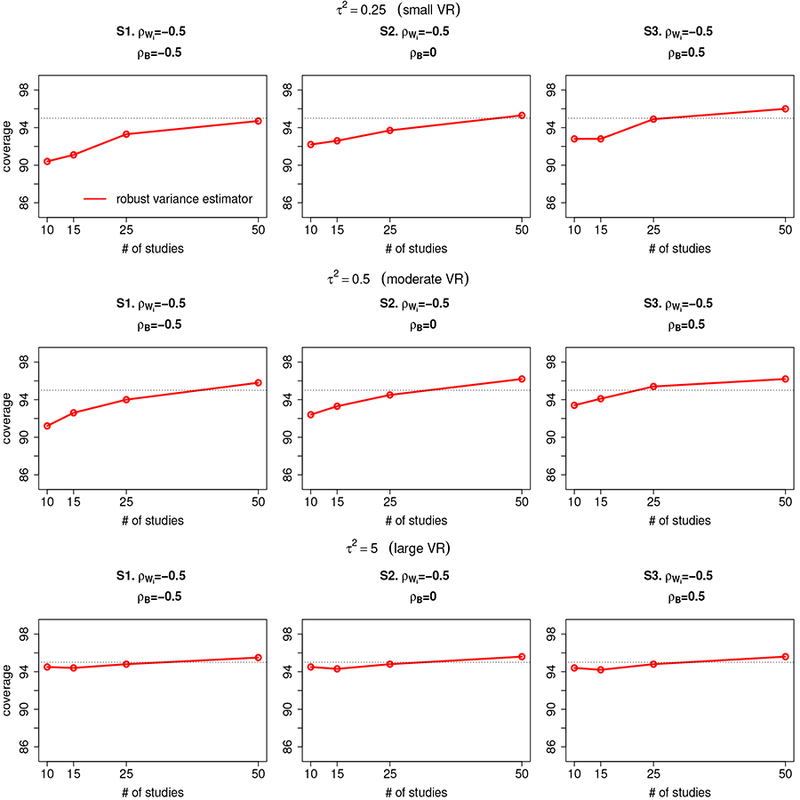
Figure 1 summarizes the coverage of confidence intervals for β₁ – β₂ estimated from Riley methods with standard variance estimator and robust variance estimator when the between-study variance ${\tau }_1^2={\tau }_2^2=0.25$. The coverage is calculated using a t distribution with m – 1 degrees of freedom, where m is the number of studies. For scenarios 1–3, when the within-study correlation (ρ_Wi) is set to be −0.5, and between-study correlation (ρ_B) is set to –0.5, 0 and 0.5, the coverage of the Riley method with standard variance estimator is similar to that with robust variance estimator (range of coverage percentage: [92%, 96%]). For scenarios 4 to 9 when either within-study correlation (ρ_Wi) or between-study correlation (ρ_B) has different values across studies, the Riley method with robust variance estimator has uniformly better coverage than that with standard variance estimator under all sample size settings (ranges of coverage percentage: [93%, 96%] for the former and [90%, 93%] for the latter). This suggests that the robust variance estimator improves the coverage of the Riley method under most of the settings considered (especially when within-study correlations and/or between study correlations vary across studies). Most importantly, the coverage of the Riley method with robust variance estimator converges to the nominal level of 95% as the number of studies increases under all scenarios.

Figure 1:

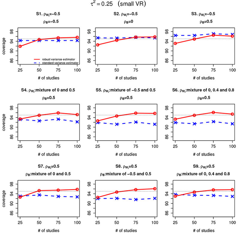
Coverage of confidence intervals for β₁ – β₂ estimated from the Riley method with standard variance estimator and the Riley method with robust variance estimator under scenarios 1–9 (denoted as S1–S9) for different settings of within-study correlation (ρ_Wi) and between-study correlation (ρ_B). The between-study variations $\left({\tau }_1^2,{\tau }_2^2\right)$ are set at 0.25, representing a relatively small between-study/within-study variation ratio (small VR). The red line refers to Riley method with robust variance estimator and the blue line refers to the Riley method with standard variance estimator.

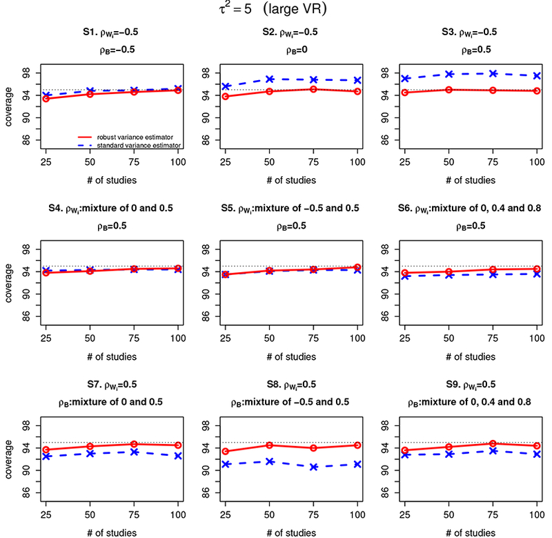
Figure 2 and 3 summarize the coverage of confidence intervals for β₁ – β₂ estimated from the Riley method with standard variance estimator and robust variance estimator when the between-study variance ${\tau }_1^2={\tau }_2^2=0.5$ and 5, respectively. The findings are similar to that in Figure 1 when the between-study variance ${\tau }_1^2={\tau }_2^2=0.25$, in that the robust variance estimator improve the coverage of the Riley method under most of the settings considered and the coverage of the Riley method with robust variance estimator converges to the nominal level of 95% as the number of studies increases under all scenarios.

Figure 2:

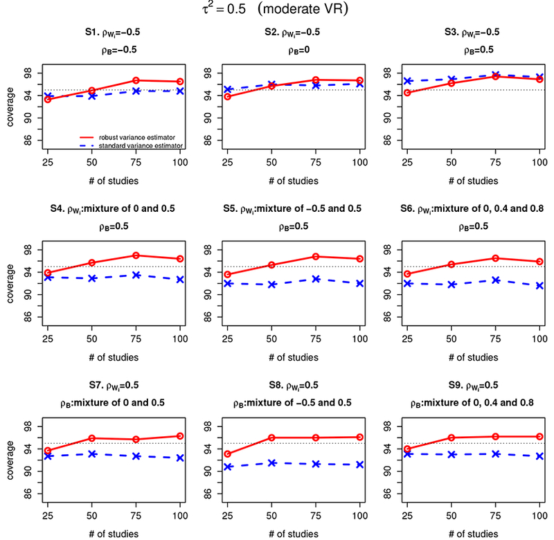
Coverage of confidence intervals for β₁ – β₂ estimated from the Riley method with standard variance estimator and the Riley method with robust variance estimator under scenarios 1–9 (denoted as S1–S9) for different settings of within-study correlation (ρ_Wi) and between-study correlation (ρ_B). The between-study variations $\left({\tau }_1^2,{\tau }_2^2\right)$ are set at 0.5, representing a relatively moderate between-study/within-study variation ratio (moderate VR). The red line refers to Riley method with robust variance estimator and the blue line refers to the Riley method with standard variance estimator.

Figure 3:

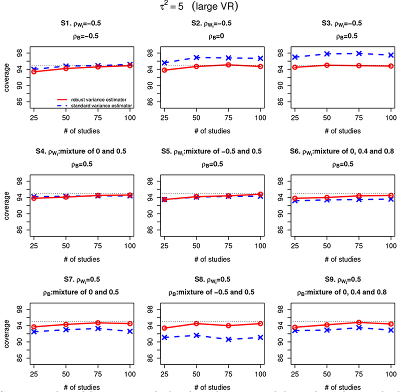
Coverage of confidence intervals for β₁ – β₂ estimated from the Riley method with standard variance estimator and the Riley method with robust variance estimator under scenarios 1–9 (denoted as S1–S9) for different settings of within-study correlation (ρ_Wi) and between-study correlation (ρ_B). The between-study variations $\left({\tau }_1^2,{\tau }_2^2\right)$ are set at 5, representing a relatively large between-study/within-study variation ratio (large VR). The red line refers to Riley method with robust variance estimator and the blue line refers to the Riley method with standard variance estimator.

Results for β₁ and β₂

Figure 4 summarizes the coverage of confidence intervals for β₁ estimated from the Riley method with standard variance estimator and with robust variance estimator when the between-study variance ${\tau }_1^2={\tau }_2^2=0.25$. We do not show results from β₂, because the performance of the two methods for β₂ are similar to that for β₁. It is interesting to observe that while improving the coverage of the function of effect sizes (e.g., β₁ – β₂), the Riley method with robust variance estimator does not improve the coverage of the individual pooled estimates(e.g., β₁ or β₂), as the coverage is very similar regardless of whether the robust or standard variance estimator is used.

Figure 4:

Coverage of confidence intervals of β₁ estimated from the Riley method with standard variance estimator and the Riley method with robust variance estimator under scenarios 1–9 (denoted as S1–S9) for different settings of marginal correlation (ρ_S)· The between-study variations $\left({\tau }_1^2,{\tau }_2^2\right)$ are set at 0.25, representing a relatively large between-study/within-study variation ratio (large VR). The red line refers to Riley method with robust variance estimator and the blue line refers to the Riley method with standard variance estimator.

3.3. Simulation results for scenarios 10 to 15

Results for β₁ – β₂

Figure 5 summarizes the coverage of confidence intervals for β₁ – β₂ estimated from the Riley method with standard variance estimator and the Riley method with robust variance estimator when the between-study variance ${\tau }_1^2={\tau }_2^2=0.25$ For scenarios 10 to 12 when the marginal correlation (ρ_S) is set to –0.5, 0, or 0.5, coverage of the Riley method with standard variance estimator is similar to that with robust variance estimator (range of CP: [92%, 96%]). For scenarios 13 to 15 when the marginal correlation (ρ_S) has different values across studies, the Riley method with robust variance estimator has uniformly better coverage than that with standard variance estimator under all sample size settings (ranges of CP: [92%, 96%] for the former and [88%, 92%] for the latter). This suggests that when the true date generating mechanism is model (2), the robust variance estimator has similar coverage performance as the standard variance estimator when the marginal correlation (ρ_S) is constant across studies, and has better coverage performance than the standard variance estimator when there is heterogeneity in marginal correlation ρ_S.

Figure 5:

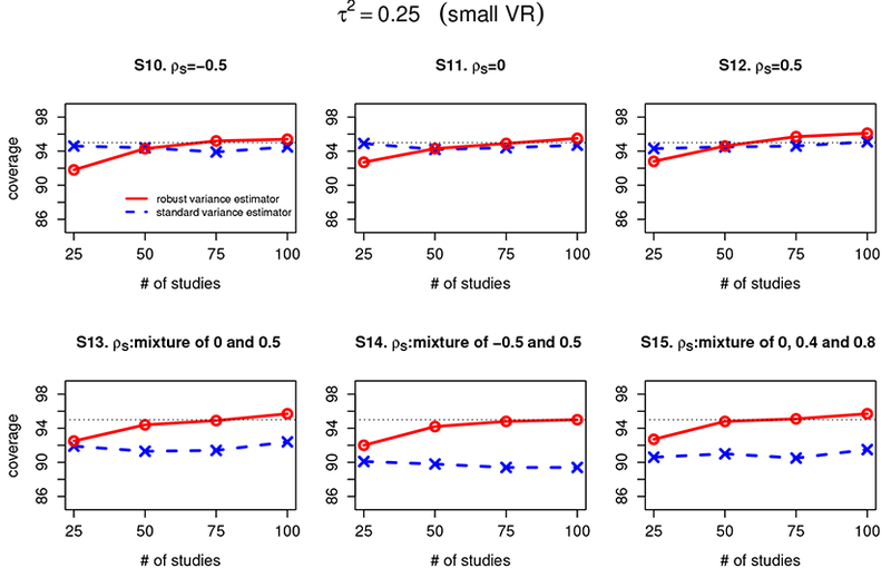
Coverage of confidence intervals of β₁ – β₂ estimated from the Riley method with standard variance estimator and the Riley method with robust variance estimator under scenarios 10–15 (denoted as S10–S15) for different settings of marginal correlation (ρ_S). The between-study variations $\left({\tau }_1^2,{\tau }_2^2\right)$ are set at 0.25, representing a relatively moderate between-study/within-study variation ratio (moderate VR). The red line refers to Riley method with robust variance estimator and the blue line refers to the Riley method with standard variance estimator.

Results for β₁ and β₂

The coverage of confidence intervals for β₁ estimated from the Riley method with standard variance estimator and with robust variance estimator when the between-study variance ${\tau }_1^2={\tau }_2^2=0.25$ are summarized in Figure S1 of the supplementary materials. Similar findings are observed from scenarios 10 to 15 as those from previous scenarios in that the coverage is very similar regardless of whether the robust or standard variance estimator is used, indicating that the Riley method with robust variance estimator does not improve the coverage of the individual pooled estimates.

3.4. Results for β₁ – β₂ when the true underlying model is multivariate t distribution

The strength of the robust variance estimators is that they allow model misspecification. In this subsection, we consider multivariate t distribution as the true underlying model for the data generation. Specifically, we consider the settings similar to Scenarios 1–3 in Section 3.1, but the random effects are generated from a multivariate t distribution. The within-study variance $s_{ij}^2$ is sampled from: subscenario T₁, a mixture of a scaled chi-squared distribution corresponding to sample size of (40, 20); subscenario T₂, a mixture of a scaled chi-squared distribution corresponding to sample size of (500, 1000); and subscenario T₃, a non-mixture chi-squared distribution corresponding to sample size of 1000.

In this situation, the Riley model is misspecified. Figure 6 summarizes the coverage of confidence intervals for β₁ – β₂ estimated from the Riley method with robust variance estimator for Scenario Τ₁. The results suggests that the robust variance estimator performs well in that the ranges of coverage percentage is [90%, 96%], even for meta-analysis with small number of studies (m = 10). We observe that the coverage of Riley method with robust variance estimator converges to the nominal level of 95% as the number of studies increases. The results for Scenario T₂ and T₃ are summarized in Table 2. Similar findings can be observed in that under all the simulation settings considered, the proposed Riley method with robust variance estimator is reasonably robust with coverage percentage close to the nominal level.

Figure 6:

Coverage of confidence intervals of β₁ – β₂ estimated from the Riley method with robust variance estimator when the true underlying distribution is bivariate t distribution. The red line refers to Riley method with robust variance estimator.

Table 2:

Results of the REML method, the Riley method with robust variance estimator (RR) and the Hedge method (RVE-JKH) in biases, empirical standard error (ESE), model based standard error (MBSE) and coverage probability (CP) for β₁, β₂ and Δ = β₁ – β₂ in 600 simulations based on data generated from multivariate t distribution. The number of studies is set to 50. The within-study variance $s_{ij}^2$ is sampled from 1) T₁: a mixture of a scaled chi-squared distribution corresponding to sample size (4, 20); 2) T₂: a mixture of a scaled chi-squared distribution corresponding to sample size (500, 1000); 3) T₃: a non-mixture chi-squared distribution corresponding to sample size of 1000.

Distribution	Method	Bias			ESEΔ	MBSEΔ	CPΔ (%)
		β1	β2	Δ
T1	REML	−0.007	−0.004	−0.003	0.150	0.138	94.8
	RS	−0.007	−0.004	−0.003	0.150	0.390	96.2
	RVE-JKH	0.003	0.003	−0.001	0.332	0.284	97.5
T2	REML	0.000	0.006	−0.006	0.153	0.155	96.5
	RS	0.000	0.006	−0.006	0.153	0.151	95.2
	RVE-JKH	0.000	0.006	0.006	0.153	0.220	99.7
T3	REML	0.001	0.004	−0.003	0.153	0.154	96.7
	RS	0.001	0.005	−0.003	0.153	0.153	95.8
	RVE-JKH	0.001	0.004	0.003	0.153	0.220	99.7

The normal distribution is commonly assumed for the random-effects in hierarchical models. However, this assumption does not always hold in practice. Using alternative random-effects distributions has been considered several times by others. Recently, Lee & Thompson (2008) explored the use of t distribution and the skew extensions as more flexible alternative for the normal assumption, and implemented the model using Markov Chain Monte Carlo methods. This method allowed for potential skewing and heavy tails in random-effects distributions and has been applied to meta-analysis and health-professional variation. When outliers or other unusual estimates are included in the analysis, the use of alternative random effect distributions has previously been proposed. Baker & Jackson (2008) proposed an alternative random-effect distributions when outliers or other unusual estimates are included in the meta-analysis and the normal assumption for random effects does not hold. Specifically, Baker & Jackson (2008) proposed a model for long-tailed distributed random effect, where the outliers are included with a reduced weight. The hierarchical approach is usually used to model the between-study variation. Recently, Baker & Jackson (2015) proposed two novel marginal distributions to model heterogeneous datasets. One of the main advantages of using the proposed marginal distributions is that the numerical integration is not needed to evaluate the likelihood. Copula models have also been used in multivariate meta-analysis. An comprehensive introduction of copula theory can be found in Nelsen (2007). Danaher & Smith (2011) described the use of copula models in multivariate settings. Recently, Kuss et al. (2014) proposed a model in the meta-analysis of diagnostic accuracy. This method linked the marginal beta-binomial distributions by bivariate copula. Given the literature above, modelling alternative random-effects models is another way to go, in addition to the uses of the robust variances.

3.5. The RVE-JKH method by Hedges et al. (2010) and Tipton (2015) vs. the proposed Riley model

Hedges et al. (2010) provided robust variance estimation (RVE) approach to combine statistically dependent effect size estimates in meta-regression, and Tipton (2015) further investigated possible approaches to adjust the robust variance estimator when the number of studies is small. To use the RVE approach, we can re-write the bivariate model in the regression form: $Y_{ij}\text{=}{X}_1{}_{{}_{ij}}{\beta }_1+X_2{}_{{}_{ij}}{\beta }_2+{ϵ}_{ij}$, for j = 1, 2 and i = 1,... ,m, where X_1ij and X_2ij are dummy variables indicating the outcome. Similarly, Y_ij = β₁ + X_2ijβ₃ + ϵ_ij allows for testing hypotheses of the form H₀ : β₃ = β₁ – β₂ = 0. It is worth mentioning that under the framework of weighted least squares, the RVE approach incorporates weights, while the RR approach does not. Another difference between the two approach is that the RVE method assumes the same between-study variation for all outcomes while the RR approach allows different between-study variation. However, since the purpose of this paper does not focus on the estimation of the between-study variance, it is of interest to compare the performance of the RVE method and that of the Riley method with robust variance estimator. As suggested by Tipton (2015), the bias reduced linearization estimator (RVE-MBB) for weighted least squares proposed by McCaffrey et al. (2001) and the jackknife estimator (RVE-JKH) proposed by MacKinnon & White (1985) perform well in a wide variety of situations. The RVE-MBB adjustment has been well implemented in the RVE analysis. However, in this work, we only implemented RVE-JKH approach because it does not require the specification of a working model. Correlated effects weights are used in RVE-JKH approach. To calculate coverage probability, we use the t-distribution with m – p degrees of freedom, as recommended by Hedges (2010) and Tipton (2015). For the REML method and the proposed Riley method with robust variance estimator, we used the t-distribution with m-1 degrees of freedom. The R codes for implementing the RVE-JKH method and calculating the coverage probability are provided in Supplementary Materials.

We have conducted additional simulation studies to compare the proposed Riley method with robust variance estimator and the RVE-JKH method. More specifically, we have included two scenarios: Scenario 1) the data are generated based on the multivariate normal distribution, and the within-study variance $s_{ij}^2$ is sampled from a scaled chi-squared distribution corresponding to sample size of 1000; and Scenario 2) the data are generated based on the multivariate t distribution, and the within-study variance $s_{ij}^2$ is sampled from: subscenario T₁ (a mixture of a scaled chi-squared distribution corresponding to sample size of 4 and 20), subscenario T₂ (a mixture of a scaled chi-squared distribution corresponding to sample size of 500 and 1000), and subscenario T₃ (a non-mixture chi-squared distribution corresponding to sample size of 1000). We consider the setting when the true model mechanism is model (1) and the between-study variance ${\tau }_1^2={\tau }_2^2=0.5$, the between-study correlation ρ_b = 0.5 and the within-study correlation ρ_Wi = –0.5. Because the simulations in previous subsections suggest the use of the proposed approach for relatively large sample, in this work, we only focus the performance comparison between the RR and RVE-JKH approaches on large sample (m = 50), while acknowledging that extending RR approach to correct for the small sample issue will be a topic of future research.

The results are summarized in Table 1 and Table 2. Under all the simulation settings considered, the three methods under comparison provide unbiased estimates of β₁, β₂ and Δ = β₁ – β₂. In regards to the coverage probability, the proposed Riley method with robust variance estimator is reasonably robust in that the range of the coverage percentage is [95.7%, 96.2%]. The RVE-JKH method provides relatively larger coverage percentage [97.5%, 99.7%]. The possible reason is that the true data generation mechanism is based on model (1), while the RVE-JKH method assumes a different working model in the meta-regression form. Therefore, it tends to provide higher model-based standard errors. In addition, we observe that the RVE-JKH method provides larger ESE compared with the REML method and the RR method for T₁ while the standard errors from the three methods are similar for T₂ and T₃. Note that for T₁, T₂ and T₃, the within-study variances are sampled from a mixture of a scaled chi-squared distribution corresponding to sample size (4, 20), (500, 1000), and a non-mixture chi-squared distribution with sample size 1000, respectively. Hence the variation of the within-study variances for T₁ are larger than those for T₂ and T₃, which is one possible reason that the ESE differs larger more for RVE-JKH vs. RR and REML in T1.

Table 1:

Results of the Riley method with robust variance estimator (RR) and the Hedge method (RVE-JKH) in biases, empirical standard error (ESE), model based standard error (MBSE) and coverage probability (CP) for β₁, β₂ and Δ = β₁ – β₂ in 600 simulations based on data generated from Normal distribution. The number of studies is set to 50. The within-study variance $s_{ij}^2$ is sampled from a scaled chi-squared distribution corresponding to sample size of 1000.

Distribution	Method	Bias				ESEΔ	MBSEΔ	CPΔ (%)
		β1		β2	Δ
Normal	RR	0.009	0.020		−0.011	0.192	0.221	95.7
	RVE-JKH	0.007	0.020		0.012	0.192	0.298	99.7

3.6. Summary

In summary, the simulation studies empirically confirm the theory of Huber (1967) that the robust variance estimator can improve the coverage of the Riley method, which is a working model, especially when functions of the pooled estimates are of interest. Since the robust variance estimator can be easily computed and has better coverage performance for β₁ – β₂ under both models (1) and (2), we recommend its use for practical investigators wishing to use the Riley method to derive functions of the pooled estimates. In terms of the individual pooled estimates (β₁ and β₂) themselves, the original Riley method with standard variance estimator and the Riley method with robust variance estimator are very similar in terms of coverage. So either variance estimator can be used for inferences. Considering all settings in the simulation studies, the RR method performs robustly no matter if the focus is hypothesis tests on β₁, β₂ or β₁ – β₂, and under both correctly model or misspecification scenarios, while we do not observe such robust performance for standard Riley method. One limitation of the proposed robust variance estimator is that it performs well when the number of studies is relatively large. As shown in Figure S2 of the supplementary materials, variances of estimated parameters may be underestimated for small number of studies (i.e., m < 15). In addition, in the case that researchers prefer a test with lower Type I errors than higher ones, small sample adjustments may be also needed for meta-analysis with moderate number of studies (i.e., m < 50). Therefore, we recommend the use of the robust method for meta-analyses with relatively large number of studies.

4. Data analysis

4.1. Effectiveness of surgery and adjuvant chemotherapy for gastric cancers

Gastric cancer, also called stomach cancer, is a cancer developing from the lining of the stomach. It is the fourth most common malignancy in the word. While the most effective treatment for gastric cancer is surgery, efforts has been made to explore different adjuvant therapies because of the recurrence after curative resection. It has been shown that postoperative adjuvant chemotherapy reduced the risk of death than surgery alone (Paoletti et al. , 2010). While overall survival (OS) is usually considered as the gold standard when investigating the effectiveness of surgery and adjuvant chemotherapy for gastric cancers, it has the disadvantage of requiring the extended follow-up period. Oba et al. (2013) conducted a meta-analysis of data from 3838 individual patients randomized in 17 trials on curatively resected gastric cancer to investigate whether disease-free survival (DFS) is a valid surrogate for OS. It is important, therefore, to study the difference between the log hazard ratio of surgery and adjuvant chemotherapy for DFS, denoted by Y_i1, and the log hazard ratio of surgery and adjuvant chemotherapy for OS, denoted by Y_i2.

Since the within-study correlations are not available, model (1) could not be applied. We therefore conduct a meta-analysis of this data using the univariate random-effects model (URMA), the Riley method with standard variance estimator and the Riley method with robust variance estimator. As shown in Table 1, for pooled estimator of individual effect sizes β₁ and β₂, the Riley method with standard variances estimator and that with robust variance estimator coincide in both point estimates and 95% confidence intervals, while the univariate meta-analysis provides greater point estimates and narrower 95% confidence intervals. The overall difference between log hazard ratio for DFS and log hazard ratio for OS (β₁ – β₂) is estimated as 0.062 (95% CI: (0.029, 0.096)) using the Riley method with standard variance estimator, and 0.062 (95% CI: (0.026, 0.098)) using the Riley method with robust variance estimator. We observe that the Riley method with robust variance estimator provides a wider 95% confidence interval than the Riley method with standard variance estimator. This observation is consistent with our simulation studies in that the model based standard errors are on average larger from robust method (Figure S3 of the supplementary materials) in terms of the function of the pooled estimates, and the robust variance estimator improves the Riley method in variance estimation. It is also worth mentioning that the Riley method with either standard variance estimator or robust variance estimator provide different results in statistical significance from that of the URMA method.

4.2. MYCN as a prognostic tumor marker in neuroblastoma

Neuroblastoma is one of the most common extracranial solid tumor occurring in children, which commonly originates from undifferentiated neural crest cells (Rossi et al. , 1994). The MYCN gene, belonging to the MYC family of transcription factors, plays an important role in making protein and formatting tissues and organs during embryonic development. The amplification of MYCN oncogene is commonly found in neuroblastoma (Bénard et al. , 2008). Riley et al. (2004) conducted a meta-analysis to investigate whether MYCN gene is in relation to the disease-free survival (DFS) and overall survival (OS) of neuroblastoma. In this meta-analysis, 17 studies reported both DFS and OS estimates, 25 studies only reported DFS, 39 studies only reported OS, and 70 studies reported neither DFS nor OS. It is important to study the difference between the log hazard ratio of MYCN for DFS, denoted by Y_i1, and the log hazard ratio of MYCN for OS, denoted by Y_i2.

We conduct meta-analyses of this data using the univariate random-effects model, the Riley method with standard variance estimator and the Riley method with robust variance estimator. The REML method is not feasible in this example due to the lack of the knowledge of the within-study correlation ρ_Wi. Note that only a proportion of studies have all outcomes reported, and the remaining studies have some of outcomes missing. Under the Missing Completely at Random assumption, we allocated very large within-study variances (e.g., 10⁶) to the missing observations, where the missing study outcomes are set to be zero (Jackson et al. , 2010). As shown in Table 2, for pooled estimator of individual effect sizes β₁ and β₂, the Riley method with standard variances estimator and that with robust variance estimator coincide in point estimates, while the univariate meta-analysis provides smaller point estimates. The overall difference between log hazard ratio for DFS and log hazard ratio for OS (β₁ – β₂) is estimated as −0.010(95% CI: (–0.341, 0.322)) using the Riley method with standard variance estimator, and −0.010 (95% CI: (–0.533, 0.514)) using the Riley method with robust variance estimator. This example again shows the discrepant standard error and confidence intervals of β₁ – β₂ for the robust and standard methods. In this example, the standard error is larger from the robust method, resulting in a wider confidence interval compared with the standard method.

5. Discussion

In this paper, we proposed a robust variance estimator to improve the Riley method with standard variance estimator for bivariate meta-analysis when within-study correlations are unknown. Our procedure uses a working covariance matrix combining the empirical version of the variance estimation in the sandwich form. The proposed method has a variety of advantages, including 1) the often unknown within-study correlations are not required when using the Riley method; 2) borrowing of strength between parameters under a missing random assumption, which is a key advantage of the multivariate approach; 3) variances for the parameters that are asymptotically correct even when the model is misspecified.

In this work, the range of the between-study and within-study correlation is set to [–0.8, 0.8], which is common in practice. However, as acknowledged by Riley et al. (2008), the performance of Riley method is unstable when the between-study correlation is close to 1 or – 1 especially when the between-study heterogeneity is relatively small. More work is needed to deal with the remaining issues in such settings. The proposed RR approach produces similar results to RVE-JKH for large sample. However, one limitation is that variances of its estimated parameters may be underestimated for small number of studies (i.e, m =< 15). As pointed by the reviewer of this paper, researchers would prefer that a test has lower Type I errors than higher in standard statistical theory. In that case, small sample adjustments may be also needed for meta-analysis with moderate number of studies (i.e., m < 50). Therefore, we recommend the use of the proposed RR approach for meta-analyses with relatively large number of studies (i.e., m ≥ 50). As inspired by Tipton (2015), improving the Riley method with robust variance estimator by incorporating small sample adjustments in both variance estimator and degrees of freedom of the t-test are future topics of interest.

Alternative methods to deal with the unknown within-study correlations have been proposed under Bayesian framework. Recently, Yao et al. (2015) developed a method to carry out Bayesian inference for multivariate meta-regression setting when the within-study correlation is missing. Specifically, in the within-study covariance matrix, the off-diagonal elements are missing, and are sampled from the appropriate full conditional distribution in a Markov Chain Monte Carlo scheme. In addition, Yao et al. (2015) proposed different structures of the within-study covariance matrix, which allow for borrowing strength across different treatment arms and trials.

There are several potential topics of future. In this work, we set the missing values at 0, assigned very large within-study variances, and use a degree of freedoms as m – 1 to calculate the coverage probability. Similar approach was used by Jackson et al. (2010). Alternatively, as in the RVE case, the missing data can be considered as unbalanced outcomes, which can affect degree of freedoms. It is of interest to see if the approach used in this work will produce better results by adjusting the degree of freedom.

In many applications study level covariates are available, such as mean age, percentage female, and year of publication. These covariates may be incorporated in the meta-analysis in order to explain some of the between-study variation. Hedges et al. (2010) provided robust variance estimation approach to combine statistically dependent effect size estimates in meta-regression. Extending Riley model with robust variance estimator to include covariates will be a topic of future research. Recently, Tipton (2015) investigated possible approaches to adjusting the robust variance estimator when the number of studies is small and found two estimators that perform better than the standard robust variance estimation approach in a wide variety of settings. Extending Riley model to adjust for the small sample size will be another topic of future research.

In addition, besides the Riley model, the robust variance estimator approach can be combined with other models for meta-analyses when the model is misspecified and the standard variance estimator is not correct (Chen et al. , 2015). Furthermore, because some models for network meta-analyses can be fitted as regression models, the proposed approach may also be useful in the network meta-analyses setting (White et al. , 2012). Very recently, Efthimiou et al. (2014) developed models for multiple correlated outcomes in a network of interventions. Specifically, they revised the models for performing multiple outcomes multivariate meta-analysis when there are only two treatment under comparison and generalized the methods for multi-arm studies. However, as acknowledged by Efthimiou et al, one major limitation for the models is that several assumptions are required when simplifying the structure of the variance-covariance matrices. The proposed robust variance estimator can be useful in this situation to correct the variance estimation.

To summarize, we develop a simple and robust variance estimator for handling correlated out-come data in meta-analyses when the full likelihood approach fails because of unknown within-study correlations and therefore a working model is required. Our method has been found to perform well when the number of studies is moderate, and provides an improved tool for all those involved in performing and interpreting multivariate meta-analyses.

Table 3:

Results of the Riley method with standard variance estimator (Riley Standard), the Riley method with robust variance estimator (Riley Robust), univariate random-effects meta-analysis (URMA), and the REML method applied to the adjuvant chemotherapy study.

method	β1(95%CI)	β2(95%CI)	β1 − β2 (95%CI)
Riley Standard	−0.219(−0.302,−0.135)	−0.281(−0.381,−0.181)	0.062(0.029, 0.096)
Robust	−0.219(−0.292,−0.145)	−0.281(−0.371,−0.191)	0.062(0.026, 0.098)
UMRA	−0.209(−0.210,−0.207)	−0.270(−0.300,−0.244)	0.061(−0.054, 0.177)*
REML	–	–	–

^*directly calculated without accounting for the correlations.

Table 4:

Results of the Riley method with standard variance estimator (Riley Standard), the Riley method with robust variance estimator (Riley Robust), univariate meta-analysis (UMRA), and the REML method applied to the MYCN study.

method	β1(95%CI)	β2(95%CI)	β1 − β2 (95%CI)
Riley Standard	1.142(0.928, 1.355)	1.152(0.903, 1.400)	−0.010(−0.341, 0.322)
Robust	1.142(0.765, 1.519)	1.152(0.738, 1.565)	−0.010(−0.533, 0.514)
UMRA	1.140(0.766,1.502)	1.147(0.750,1.545)	−0.008(−0.315, 0.299)*
REML	-	-	-

^*directly calculated without accounting for the correlations.

References

- Baker Rose, & Jackson Dan. 2008. A new approach to outliers in meta-analysis. Health care management science, 11(2), 121–131. [DOI] [PubMed] [Google Scholar]
- Baker Rose, & Jackson Dan. 2015. New models for describing outliers in meta-analysis. Research synthesis methods. [DOI] [PMC free article] [PubMed] [Google Scholar]
- Bénard Jean, Raguénez Gilda, Kauffmann Audrey, Valent Alexander, Ripoche Hugues, Joulin Virginie, Job Bastien, Danglot Giséle, Cantais Sabrina, Robert Thomas, et al. . 2008. Mycn-non-amplified metastatic neuroblastoma with good prognosis and spontaneous regression: a molecular portrait of stage 4s. Molecular oncology, 2(3), 261–271. [DOI] [PMC free article] [PubMed] [Google Scholar]
- Berkey CS, Antczak-Bouckoms A, Hoaglin DC, Mosteller E, & Pihlstrom BL. 1995. Multiple-outcomes meta-analysis of treatments for periodontal disease. Journal of dental research, 74(4), 1030–1039. [DOI] [PubMed] [Google Scholar]
- Borenstein M, Hedges LV, Higgins JPT, & Rothstein HR 2009. Introductionto meta-analysis. Wiley Online Library. [Google Scholar]
- Chen Yong, Hong Chuan, & Riley Richard D. 2015. An alternative pseudolikelihood method for multivariate random-effects meta-analysis. Statistics in medicine, 34(3), 361–380. [DOI] [PMC free article] [PubMed] [Google Scholar]
- Danaher Peter J, & Smith Michael S. 2011. Modeling multivariate distributions using copulas: applications in marketing. Marketing science, 30(1), 4–21. [Google Scholar]
- Daniels MJ, & Hughes MD 1997. Meta-analysis for the evaluation of potential surrogate markers. Statistics in medicine, 16(17), 1965–1982. [DOI] [PubMed] [Google Scholar]
- Diggle Peter, Liang Kung-Yee, & Zeger Scott L. 1994. Longitudinal data analysis. [Google Scholar]
- Efthimiou Orestis, Mavridis Dimitris, Riley Richard D, Cipriani Andrea, & Salanti Georgia. 2014. Joint synthesis of multiple correlated outcomes in networks of interventions. Biostatistics, kxu030. [DOI] [PMC free article] [PubMed] [Google Scholar]
- Gasparrini Antonio, & Gasparrini Maintainer Antonio. 2014. Package mvmeta.Hartung, J., Knapp, G., & Sinha, B.K. 2011 Statistical meta-analysis with applications. Vol. 738 Wiley-Interscience. [Google Scholar]
- Hedges Leon V, Tipton Elizabeth, & Johnson Matthew C. 2010. Robust variance estimation in meta-regression with dependent effect size estimates. Research synthesis methods, 1(1), 39–65. [DOI] [PubMed] [Google Scholar]
- Huber PJ 1967. The behavior of maximum likelihood estimates under nonstandard conditions . Pages 221.– of: Proceedings of the fifth berkeley symposium on mathematical statistics and probability, vol. 1. [Google Scholar]
- Ishak K Jack, Platt Robert W, Joseph Lawrence, & Hanley James A. 2008. Impact of approximating or ignoring within-study covariances in multivariate meta-analyses. Statistics in medicine, 27(5), 670–686. [DOI] [PubMed] [Google Scholar]
- Jackson D, Riley R, & White IR 2011a. Multivariate meta-analysis: Potential and promise. Statistics in medicine, 30(20), 2481–2498. [DOI] [PMC free article] [PubMed] [Google Scholar]
- Jackson D, Riley R, & White IR 2011b. Multivariate meta-analysis: Potential and promise. Statistics in medicine, 30(20), 2481–2498. [DOI] [PMC free article] [PubMed] [Google Scholar]
- Jackson Dan, White Ian R, & Thompson Simon G. 2010. Extending dersimonian and laird’s methodology to perform multivariate random effects meta-analyses. Statistics in medicine, 29(12), 1282–1297. [DOI] [PubMed] [Google Scholar]
- Kuss Oliver, Hoyer Annika, & Solms Alexander. 2014. Meta-analysis for diagnostic accuracy studies: a new statistical model using beta-binomial distributions and bivariate copulas. Statistics in medicine, 33(1), 17–30. [DOI] [PubMed] [Google Scholar]
- Lee Katherine J, & Thompson Simon G. 2008. Flexible parametric models for random-effects distributions. Statistics in medicine, 27(3), 418–434. [DOI] [PubMed] [Google Scholar]
- Liang Kung-Yee, Zeger Scott L, & Qaqish Bahjat. 1992. Multivariate regression analyses for categorical data. Journal of the royal statistical society. series b (methodological), 3–40. [Google Scholar]
- Liang KY, & Zeger SL 1986. Longitudinal data analysis using generalized linear models. Biometrika, 73(1), 13–22. [Google Scholar]
- Lin DY. 1994. Cox regression analysis of multivariate failure time data: the marginal approach. Statistics in medicine, 13(21), 2233–2247. [DOI] [PubMed] [Google Scholar]
- MacKinnon James G, & White Halbert. 1985. Some heteroskedasticity-consistent covariance matrix estimators with improved finite sample properties. Journal of econometrics, 29(3), 305–325. [Google Scholar]
- McCaffrey Daniel F, Bell Robert M, & Carsten H Botts. 2001. Generalizations of bias reduced linearization. In: Proceedings of the survey research methods section. [Google Scholar]
- Nam IS, Mengersen K, & Garthwaite P 2003. Multivariate meta-analysis. Statistics in medicine, 22(14), 2309–2333. [DOI] [PubMed] [Google Scholar]
- Nelsen Roger B. 2007. An introduction to copulas. Springer Science & Business Media. [Google Scholar]
- Oba Koji, Paoletti Xavier, Alberts Steven, Bang Yung-Jue, Benedetti Jacqueline, Bleiberg Harry, Catalano Paul, Lordick Florian, Michiels Stefan, Morita Satoshi, et al. . 2013. Disease-free survival as a surrogate for overall survival in adjuvant trials of gastric cancer: a meta-analysis. Journal of the national cancer institute, djt270. [DOI] [PMC free article] [PubMed] [Google Scholar]
- Paoletti Xavier, Oba Koji, Burzykowski Tomasz, Michiels Stefan, Ohashi Yasuo, Pignon Jean-Pierre, Rougier Philippe, Sakamoto Junichi, Sargent Daniel, Sasako Mitsuru, et al. . 2010. Benefit of adjuvant chemotherapy for resectable gastric cancer: a meta-analysis. Jama: the journal of the american medical association, 303(17), 1729–1737. [DOI] [PubMed] [Google Scholar]
- Riley RD, Thompson JR, & Abrams KR 2008. An alternative model for bivariate random-effects meta-analysis when the within-study correlations are unknown. Biostatistics, 9(1), 172–186. [DOI] [PubMed] [Google Scholar]
- Riley RD, Price MJ, Jackson D, Wardle M, Gueyffier F, Wang J, Staessen JA, & White IR. 2014. Multivariate meta-analysis using individual participant data. Research synthesis methods. [DOI] [PMC free article] [PubMed] [Google Scholar]
- Riley Richard D, Sutton Alex J, Abrams Keith R, & Lambert Paul C. 2004. Sensitivity analyses allowed more appropriate and reliable meta-analysis conclusions for multiple outcomes when missing data was present. Journal of clinical epidemiology, 57(9), 911–924. [DOI] [PubMed] [Google Scholar]
- Rossi Anne R, Pericle F, Rashleigh S, Janiec J, & Djeu JY. 1994. Lysis of neuroblastoma cell lines by human natural killer cells activated by interleukin-2 and interleukin-12. Blood, 83(5), 1323–1328. [PubMed] [Google Scholar]
- Tipton Elizabeth. 2015. Small sample adjustments for robust variance estimation with metaregression. Psychological methods, 20(3), 375. [DOI] [PubMed] [Google Scholar]
- Van Houwelingen Hans C, Arends Lidia R, & Stijnen Theo. 2002. Advanced methods in metaanalysis: multivariate approach and meta-regression. Statistics in medicine, 21(4), 589–624. [DOI] [PubMed] [Google Scholar]
- Varin C 2008. On composite marginal likelihoods. Asta advances in statistical analysis, 92(1), 1–28. [Google Scholar]
- Wei Yinghui, & Higgins Julian. 2012. Estimating within-study covariances in multivariate meta-analysis with multiple outcomes. Statistics in medicine. [DOI] [PMC free article] [PubMed] [Google Scholar]
- White Halbert. 1982. Maximum likelihood estimation of misspecified models. Econometrica: Journal of the econometric society, 1–25. [Google Scholar]
- White Ian R, Barrett Jessica K, Jackson Dan, & Higgins Julian. 2012. Consistency and inconsistency in network meta-analysis: model estimation using multivariate meta-regression. Research synthesis methods, 3(2), 111–125. [DOI] [PMC free article] [PubMed] [Google Scholar]
- White IR 2011. Multivariate random-effects meta-regression: updates to mvmeta. Stata journal, 11(2), 255–270. [Google Scholar]
- Yao Hui, Kim Sungduk, Chen Ming-Hui, Ibrahim Joseph G, Shah Arvind K, & Lin Jianxin. 2015. Bayesian inference for multivariate meta-regression with a partially observed within-study sample covariance matrix. Journal of the american statistical association, 110(510), 528–544. [DOI] [PMC free article] [PubMed] [Google Scholar]
Associated Data
This section collects any data citations, data availability statements, or supplementary materials included in this article.