Thrust and torque force analysis in the drilling of aramid fibre-reinforced composite laminates using RSM and MLPNN-GA

Abstract

Aramid Fibre Reinforced Plastic composites are difficult to be drilled due to anisotropic material properties. Currently, soft computing techniques are used as alternatives to conventional mathematical models, which is robust and can deal with inaccuracy and uncertainty. In this paper, drilling of Aramid Fibre Reinforced Plastics (AFRPs) was carried out using Taguchi L54 experimental layout. Drilling tool used in this experiment was solid carbide. The purpose of this study was to find optimum combination of drilling parameters to obtain minimum thrust and torque force to reduce the delamination. Also, this paper proposed a prediction model of Multilayer Perception Neural Network optimized by Genetic Algorithm (MLPNN-GA). Moreover, RSM technique was used to evaluate the influence of process parameters (spindle speed, feed rate, drill point angle and drill diameter on thrust force and torque. The prediction capability of both RSM and MLPNN-GA was compared with Response optimizer for thrust force and torque. The investigation demonstrated that drill point angle is the primary factor affecting thrust force and drill diameter influences the torque force on the drill bit. Overall, this study recommends the use of high speed and low feed combination and drill point angles of 90°–118° to reduce the delamination of the materials in the drilling of AFRP composites.

1. Introduction

The materials used in construction, aerospace, automotive industries, etc. need to have high specific stiffness, high damping, high strength, high thermal resistance and low thermal expansion. Further, these materials should be corrosion & wear resistant and dimensionally stable. Composites such as Aramid Fibre Reinforced Plastics/Polymers (AFRP) exhibit such distinct properties and hence find broad applications in cryogenics, sports equipment, ropes & cables, ballistic applications, building construction, breaks, armor, aerospace, etc. Composite materials are two or more chemically different constituents combined synergistically and macroscopically to yield a useful material that is different in physical form and chemical composition of the parent materials. The purpose of having two or more constituents is to get rid of the inferior properties of the constituents and to gain benefits of the superior features of all the constituents. However, due to the presence of the two or more different phases AFRP composites pose various kinds of machining problems. Thus, the machining mechanism of composite materials is different from that of the homogeneous conventional materials [1, 2, 3, 4].

The distinctive difficulties like delamination, fibre pull out, melting of the matrix, adhesion of materials to drill etc., are found while drilling of AFRP composites. These failures adversely affect the quality of the AFRP composites. Lamination, resin type, fibres, reinforcing materials all these factors also significantly modify the properties of AFRP composites. Therefore, it is necessary to control the factors affecting the drilling of AFRP composites [4, 5, 6, 7, 8]. Various researchers used different and innovative ways to control the factors affecting the drilling of composites.

Bishop and Gindy, 1990 [4] performed an investigation on drilling of ballistic Kevlar composites and concluded that drill point angle influenced thrust force and was maximum at 180°. The removal of drill web achieved a further reduction in angle and increase in the rake angle reduced the torque, varying point angle had a lesser effect on torque. Di Ilio et al., 1991 [6] concluded that interfaces between the laminate and inhomogeneity inside single lamina were responsible for oscillations of thrust force in the drilling of aramid composites. High friction forces influenced torque force at the lands of a twist drill. Horrigan, 1998 [7] conducted a study on hole drilling in Kevlar composites. The study showed that under the cryogenic condition, modified drill bit produced a greater thrust force than the usual drill bit at ambient temperature. Larger the thrust force, higher the delamination and by use of backing plate the delamination reduced. A laser drilling of aramid and glass/epoxy composites were performed on printed wiring boards by Hirogaki et al., 2001 [8]. Liu et al., 2012 [9] conducted a review of composite laminates. They revealed that vibration-assisted twist drilling and high-speed drilling reduced the delamination induced drilling more than conventional method. Among various drill bits, twist drill bit was the most studied drill bit. They also inferred that during low feed rate, delamination occurred. In practical situations, peel up delamination was less severe than push-out delamination and even the thrust force was in direct relationship with delamination. Feito et al., 2016 [10] studied the influence of tool wear and special cutting geometry when drilling the woven CFRP composites. They concluded that low feed rate and high cutting speed reduced the drilling induced delamination. Feed rate is the most influential factor for both thrust force and delamination.

Karpat et al., 2012 [11] performed experiments on drilling of thick fabric woven CFRP laminates using double point angle drills. The study showed that increasing feed rate and rotational speed protected the diamond coated carbidedrill bit and also improved the hole quality. It was noted that properties of CFRP material, the rigidity of machine tools and drilling geometry also play an essential role. Palanikumar, 2011 [12] experimented GFRP composites using Spur and Brad drill and established that low feed rate and high spindle speed are necessary to reduce delamination and also it had an effect on grey relational grade. It was observed that feed rate is the most influential factor. Sunny et al., 2014 [13] carried out experiments on GFRP composites by Taguchi Method L25 using three different tools viz., twist drill, end mill and Kevlar drill. The study revealed that feed rate is the most influential parameter and high spindle speed and low feed rate decreased the delamination. In the case of kevlar drill, observed delamination was less. Krishnaraj et al., 2012 [14] experimented with the high-speed drilling of CFRP laminates. They inferred that feed rate had a more significant influence on the diameter of the hole, push out delamination and thrust force. The circularity of the hole was affected by spindle speed and feed rate. The spindle speed did not have much influence on peel-up delamination. Mohan et al., 2005 [15] carried out experiments with glass–fibre polyester reinforced composites and noted that minimum thrust force could be obtained by lower feed rate, less specimen thickness and drill diameter, and higher speed. Also, minimum torque force could be obtained by higher speed, medium feed, low specimen thickness and high drill diameter. Tsao and Hocheng, 2004 [16] performed Taguchi analysis on various drill bits of composite material and found that feed rate and drill diameter made the most significant contribution. Twist drill caused more delamination than candlestick drill and saw drill. Tsao and Chiu, 2011 [17] carried out experiments on the drilling of CRFP composite laminate using compound core-special drills. Feed rate, cutting speed and inner drill type were the most affecting factors; feed rate and high negative cutting velocity produced a low thrust force in drilling the composite material. Khashaba et al., 2010 [18] conducted an experiment on machinability analysis in drilling the woven GFR/epoxy composites and noted that as the feed rate and drill diameter increased, thrust force also increased. The increase in cutting speed also increased the surface roughness. Rajamurugan et al., 2013 [19] conducted experiments on glass fibre reinforced polyester composites and revealed that rise in drill diameter increased the delamination factor. Also, increase in fibre orientation factor increased the delamination. Zarif et al., 2013 [20] experimented with glass/epoxy laminates. They revealed that feed rate and drill point angle had a significant effect on delamination factor. Kilickap, 2010 [21] conducted experiments on GFRP composite at drill point angles of 118° and 135° and concluded that feed rate is a most important factor and drill point angle at 118° produced less damage and delamination. Karnik et al., 2008 [22] conducted a study on high-speed drilling of CRFP using artificial neural network model and concluded that increase in cutting speed and decrease in feed rate reduced the drilling induced delamination. Kumar and Ganta, 2013 [23] experimented with the drilling of GFRP composite using Taguchi method. Their study indicated that low thrust force could be obtained by lower speed, medium feed rate, chisel edge (0.8 mm) and point angle of 90°. Whereas optimum torque can be achieved by lower speed, high feed rate, 1.6 mm chisel edge and point angle of 95°. Gaitonde et al., 2008 [24] showed that apart from spindle speed, drill point angle and low feed minimized the delamination in drilling of CFRP composites. Wang et al., 2013 [25] experimented tool wear of coated drills in drilling the CFRP composites and found that all drill types showed an ordinary wear of edge rounding wear. Tsao et al., 2012 [26] showed delamination during drilling of the composite and proposed a model delamination reduction by backup force. The results revealed that delamination could be reduced significantly with a low-level backup force and diamond coated drill significantly decreased edge rounding wear. Also, critical thrust force [27] and critical feed predictions models [28] on composites were developed and numerical predictions were derived on CFRP composites [29].

From the above literatures it can be inferred that Taguchi method and multi-variable regression models were conventionally used by researchers to perform the analysis of experiments. As computerized models were tolerant of uncertainty, imprecision, approximation and also evolving in nature, they replaced mathematical and analytical models. These are known as soft computing techniques, example: Neural Networks, Genetic algorithm, Fuzzy logic, etc. Tsao, 2008 [30] showed that Radial Bias Function Network (RBFN) predicted thrust force values much better than multi-variable linear regression model. Significant developments of intelligent systems have been inspired by the neural network which is a function of neurons and dendrites in the brain of a human being. Artificial Neural Network (ANN) can be used to solve problems related to pattern recognition, optimization, clustering, predictions, etc. [31]. ANNs find their application in the fields like finding tunnel settlements and openings in the underground, excavations, liquefaction, analyzing properties of soil and their behavior etc. [32]. ANNs are data-driven methods, which can approximate complex non-linear relationships using non-linear mapping by processing data without the prior knowledge of the model structure. They can handle incomplete and unclear data and can learn from examples and tolerate faults in the data. ANN receives a new piece of information; interconnections are adjusted to avoid losing the old data [33, 34, 35]. Dini, 2007 [36] used the feed-forward neural network to predict delamination in drilling of GFRP composite, and the results were excellent regarding the performance. Enemuoh et al., 2001 [37] developed the technique for drilling of carbon fibre reinforced thermosets using the nonlinear sequential quadratic-programming algorithm to analyze the drilling parameters. They also inferred that high spindle speed and low feed rate produced delamination free drill and good surface finish. The study indicated that for epoxy composites, the best drill point angle is 118°.

ANN method often falls into the trap of local convergence, and genetic algorithm (GA) gives the global searching ability by finalizing the first weight and bias of the ANN. This global searching ability of GA improves the accuracy of ANN and converges more quickly [38]. Saravanana M., et al., 2012 [39] carried out multi-objective optimization of drilling parameters using GA. The variation of parameters was approached by both GA and finite element method and concluded that GA approach was much better than the finite element method. Krishnaraj et al., 2012 [40] used GA (multi-objective optimization) to find optimum cutting conditions for defect-free drilling.

It is clear from the literature reviews that studies related to drilling of the composites with artificial neural network (ANNs) and genetic algorithm will give better prediction than the other available regression models. In addition, the literature reviews highlighted that most of the research work was carried on CFRP and GFRP composites, and there is no considerable work reported on the AFRP composites. Similarly, integration of GA and MLPNN was not discussed widely in the literatures. Hence, in the present work, an attempt was made to find optimum values of thrust and torque force for drilling of AFRP composites using MLPNN-GA approach. Also, an attempt had been made to analyze the process parameters of AFRP composites namely drill diameter, drill point angle, feed rate and spindle speed using Taguchi analysis. The drill bit angles of 90° and 118° and drill diameters of 6 mm, 8 mm, and 10 mm were selected in the present work. The feed rates of 50, 75, 100 mm/min and spindles speeds of 600, 900, 1200 rpm were employed in this work. The drilling process parameters (point angle, drill diameter, speed, and feed) were optimized using ANOVA, RSM, and GA-MLPNN to minimize thrust and torque force to obtain higher quality drilled holes with minimum delamination of composites.

2. Materials & methods

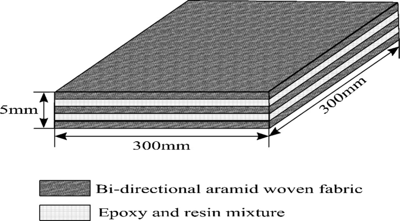
Aramid Fibre Reinforced Plastic (AFRP) specimen was prepared using the Hand-Layup method. The mould was of medium size and coated with anti-adhesive to prevent the specimen from sticking to the mould. Gel coating was applied to form the primary surface layer. Grinders were used at the top and bottom of mould plate to get the excellent surface finish. Bi-directional aramid woven fibres were cut as per the mould size and placed on the surface of the mould. The total thickness of the sheet was 1.2 mm. Matrix epoxy resin Lapox B-11 mixed thoroughly with hardener AP5140, was poured onto to the surface of woven fabric which was already placed in the mould. Epoxy was uniformly spread using the brush. The second layer of the woven fabric mat of same thickness was placed in the middle of the mould; mild pressure was applied to remove the trapped air as well as excess epoxy. Again, the resin and hardener were employed, one more layer of aramid fabric was placed at the top. The same process was repeated for other layers also. The top mould plate was kept and the pressure was applied to the specimen and cured for 48 hours at atmospheric conditions. Later, the mould was opened and AFRP was taken out of the mould. The developed composite dimensions chosen for the study were 300 mm × 300 mm × 5 mm, as shown in Fig. 1.

Fig. 1.

Laminate layout.

2.1. Details of the workpiece

In the present study, a 5 mm thickness Aramid Fibre Reinforced Plastic (AFRP) composite was prepared by hand lay-up method. The matrix epoxy resin lapox B-11, and hardener AP5140 properties are shown in Tables 1 and 2. Similarly, the properties of reinforcement material – bi-directional aramid woven fabric are displayed in Table 3.

Table 1.

Properties of epoxy resin.

Property	Unit	Test method	Value
Appearance	-	Visual	Clear viscous liquid
Color	APHA	ASTM D 1209 D 5386	Max. 100
Epoxy value	Eq./kg	ASTM D 1652	5.25–5.45
Viscosity at 25 °C	mPa-s	ASTM D 2196	10000–12000
Hydrolysable chlorine	%	ASTM D 1726	Max. 0.1

Table 2.

Properties of hardener.

Property	Value
Appearance (Visual)	Clear pale colored viscous liquid
Odor	Amine
Color (Gardner, ASTM D 1544)	10 max
Viscosity at 40 °C DIN 53015 (ISO 12058)	3000–6000 mPa-s
Density at 25 °C (ASTM D 1457)	0.95–0.97 kg/l
Non-volatiles	Solvent free
Amine numbers (ISO 9702)	370–400 mg KOH/g
Amine hydrogen equivalent wt.	95

Table 3.

Properties of reinforcement.

“Customary” (inch-pound) units
Specific density lb/in3	Tenacity 103 psi	Modulus 106 psi	Break elongation	Specific tensile strength 106 in.	CTE 10−6/°F	Decomposition temperature
						(°F)	(°C)
0.052	424	10.2	3.6	8.15	−2.2	800–900	(427–482)
0.052	435	16.3	2.4	8.37	−2.7	800–900	(427–482)

2.2. Machining set-up

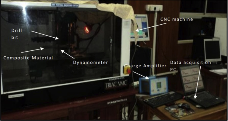
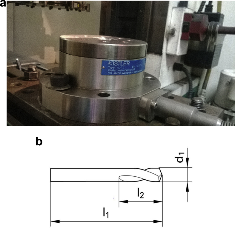
The machining setup used for drilling of AFRP is Triton VMC three-axis milling machine and is suitable for machining the wax, plastics, acrylics, copper, aluminum, composites, and steel as shown in Fig. 2. It has inbuilt PC controller, and solid carbide drill bits of 6 mm, 8 mm, 10 mm diameter were used to perform the drilling trials. The specification of solid carbide drill bit is shown in Fig. 3b and Table 4. Thrust force and torque developed during drilling operations were measured using KISTLER dynamometer as shown in Fig. 3a. Charge amplifier produces a voltage output proportional to the force input, and the generated voltage is measured using Data Acquisition PC.

Fig. 2.

Triton VMC (Vertical milling centre).

Fig. 3.

(a) KISTLER dynamometer. (b) Solid carbide drill bit.

Table 4.

Solid carbide drill bit specifications.

Drill point angle	Diameter	Shank dia.	OAL	Flute length	Cutting depth	Flutes	Shank	Coating
	d1	d2	l1	l2	tMax
	(mm)	(mm)	(mm)	(mm)	(mm)
90 degrees	6.000	6.000	66.00	16.00	7.00	2	Straight	Bright
	8.000	8.000	79.00	21.00	9.00	2	Straight	Bright
	10.000	10.000	89.00	25.00	10.00	2	Straight	Bright
118 degrees	6.000	6.000	83.00	51.00	-	Spiral	-	Bright
	8.000	8.000	92.00	60.00	-	Spiral	-	Bright
	10.000	10.000	114.00	73.00	-	Spiral	-

3. Methodology

3.1. Taguchi method

AFRP values were analyzed with the Taguchi method, and this method allows to perform a pair of combinations of tests. In this study, drill point angle, drill diameter, spindle speed and feed rate were selected. The drill parameters and levels are shown in Table 5. The experiments were conducted according to Taguchi's L₅₄ Orthogonal Array, shown in Table 6. The drill diameter, speed, and feed have three levels, and drill point angle had two levels. In this work, Taguchi's L₅₄ (2¹*3³) orthogonal array was considered, as the L₈ (2¹*3³) array was insufficient to handle the data. In the current study, fifty-four sets of experiments were conducted using standard design matrix of factorial design. Drill parameters concerning thrust and torque forces were measured using S-N ratio. There are three types of Taguchi's S-N ratio variations as given below. In the present work, Smaller is better was chosen as the variation.

• (i)Larger is better: It is used when a more substantial value is desired as indicated in equation (1).

$$S/Nratio\left(\mathrm{\eta }\right)=-10{\log }_{10}\frac{1}{n}\sum _{i=0}^n\frac{1}{y_i^2}$$ (1)

where n is the number of replications and y_i is observed response value.

• (ii)Nominal is the best: It is used when variation about the nominal or target value is minimum as shown in equations (2) and (3).

$$S/Nratio\left(\mathrm{\eta }\right)=10{\log }_{10}\frac{{\mu }^2}{{\sigma }^2}$$ (2)

$$S/Nratio\left(\mathrm{\eta }\right)=-10{\log }_{10}{\sigma }^2$$ (3)

where μ is the mean and σ is the variance.

• (iii)Smaller is better: It is used when the smaller value is desired. The “smaller is the better” means minimizing the response and the target value is non-negative with zero [15].

$$S/Nratio\left(\mathrm{\eta }\right)=-10{\log }_{10}\frac{1}{n}\sum _{i=0}^n{y}_i^2$$ (4)

Table 5.

Factor information.

Factor	Type	Level	Values
DA (Drill Point Angle)	Fixed	2	90°, 118°.
DD (Drill Diameter)	Fixed	3	6 mm, 8 mm, 10 mm.
SPEED (Spindle Speed)	Fixed	3	600 rpm, 900 rpm, 1200 rpm.
FEED (Feed Rate)	Fixed	3	50 mm/min, 75 mm/min, 100 mm/min.

Table 6.

Taguchi's L₅₄ (2¹*3³) orthogonal array.

Test no.	DA	DD	SPEED	FEED	Test no.	DA	DD	SPEED	FEED
1	90	6	600	50	28	118	6	600	50
2	90	6	600	75	29	118	6	600	75
3	90	6	600	100	30	118	6	600	100
4	90	6	900	50	31	118	6	900	50
5	90	6	900	75	32	118	6	900	75
6	90	6	900	100	33	118	6	900	100
7	90	6	1200	50	34	118	6	1200	50
8	90	6	1200	75	35	118	6	1200	75
9	90	6	1200	100	36	118	6	1200	100
10	90	8	600	50	37	118	8	600	50
11	90	8	600	75	38	118	8	600	75
12	90	8	600	100	39	118	8	600	100
13	90	8	900	50	40	118	8	900	50
14	90	8	900	75	41	118	8	900	75
15	90	8	900	100	42	118	8	900	100
16	90	8	1200	50	43	118	8	1200	50
17	90	8	1200	75	44	118	8	1200	75
18	90	8	1200	100	45	118	8	1200	100
19	90	10	600	50	46	118	10	600	50
20	90	10	600	75	47	118	10	600	75
21	90	10	600	100	48	118	10	600	100
22	90	10	900	50	49	118	10	900	50
23	90	10	900	75	50	118	10	900	75
24	90	10	900	100	51	118	10	900	100
25	90	10	1200	50	52	118	10	1200	50
26	90	10	1200	75	53	118	10	1200	75
27	90	10	1200	100	54	118	10	1200	100

3.2. Analysis of variance (ANOVA)

ANalysis Of VAriance (ANOVA) is used to find the significance of each value in AFRP composites study. The variance seen in variables is partitioned into different parts or components based on the deviation and hence the name ANalysis of VAriance (ANOVA). ANOVA compares different factor levels with response to access the importance of one or more factors. General linear model (GLM) approach was used in this experiment, and it uses least square regression method to describe the statistical relationship between one or more factors and the response variable. In this work, P-values were associated with Fischer's F-test. The model is said to be adequate when F-ratio value is more than the standard tabulated F-ratio value at a confidence interval of 95%.

3.3. Response surface method (RSM)

In this work, Response Surface Method (RSM) was used to compute 3D surface and contour plots of AFRP drill parameter variations. RSM is a collection of statistical and mathematical procedures for figuring out the relationship between the responses to given problems and several factors affecting the problem. Proper planning of experiments was necessary to construct the mathematical model based on experimental data. For this reason, a second-degree non-linear polynomial regression was used to describe the relationship between drilling process parameters of AFRP and thrust and torque force, as shown in equation (5). This equation is the representation of the regression line in algebraic format. In the current study, Central Composite Design (CCD) approach was used for RSM. The chosen values before the experiment: number of cube points was 32; center points in the cube was 8; axial points was 10; center points in axial was 4 and the value of alpha for RSM was 2.366. The commercially available MINITAB software was used for the RSM study. By default, Minitab uses coded units to perform the RSM operation. Then these coded coefficients were converted to un-coded coefficients by Minitab software. Equation (5) is the obtained regression equation in un-coded units.

Td = βο + β₁ DA + β₂ DD + β₃ SPEED + β₄ FEED + β₁₁ DA*DA + β₂₂ DD*DD + β₃₃ SPEED*SPEED + β₄₄ FEED*FEED + β₁₂ DA*DD + β₁₃ DA*FEED + β₁₄ DA*FEED + β₂₃ DD*SPEED + β₂₄ DD*FEED + β₃₄ SPEED*FEED (5)

where, Td is the thrust or torque force, β_ο is the constant, β₁…β₄₄ is the regression coefficients of the model to be determined. DA, DD…, SPEED*FEED are the values of the term.

3.4. Modeling of genetic algorithm and neural network

The diversity of data can enhance the learning and generalization ability of neural network which can be obtained with a reduction in the similarity of data. Therefore, the data was normalized within the range [0, 1] for both input and output data using equation (6).

$$x_n=\frac{y_{\mathit{max}}-y_{\mathit{min}}}{x_{\mathit{max}}-x_{\mathit{min}}}\left(x-x_{\mathit{min}}\right)+y_{\mathit{min}}$$ (6)

where, x_n is the normalized value of variable x; x_max and x_min are the maximum and minimum of x, respectively; y_max and y_min are the maximum and minimum of the normalized targets, respectively.

3.4.1. Multilayer perceptron neural network (MLPNN)

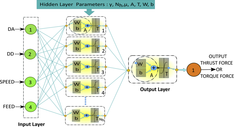
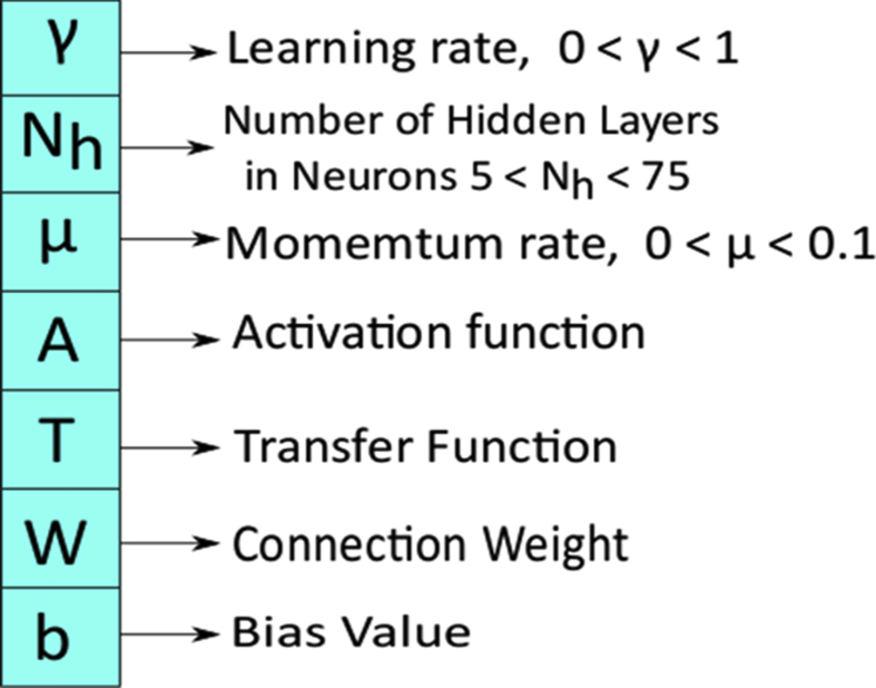
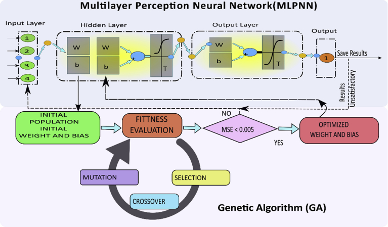
This technique was used to predict the thrust and torque force in the drilling of AFRP composites. MLPNN consists of four neurons in the input layer corresponding to four input process parameters (SPEED: spindle speed, FEED: feed rate, DA: point angle and DD: drill diameter). The output layer consists of a single neuron which is either thrust force or torque force as output process parameters. A single hidden layer with N_h (number of hidden neurons) was used in this work as shown in Fig. 4. These also hold weights and biases in the hidden layer (W_ij, b_ij) and an output layer (W_jk, b_jk). Sigmoidal activation function was selected as activation function for both inputs and outputs. For training purpose, back-propagation (BP) algorithm was used in MLPNN. In this study, gradient descent with momentum and adaptive learning rate back propagation (gdx) was used due to its ability to update weights and biases. Also, other factors like learning rate (γ) and momentum rate (μ) were chosen as shown in Fig. 5. The Performance of MLPNN was validated through MSE (Mean Square Error) as given in equation (7). The learning rate parameter was used during the adjustment of weights and biases to control the speed of learning algorithm and activation functions (hyperbolic tangent sigmoid and log-sigmoid). Similarly, the momentum rate and number of hidden neurons also greatly affect the outcome of MLPNN. In this work, MATLAB – NNTOOL was used to perform the neural network analysis. The selection process of number of data points for training, testing and validation will be carried out automatically in NNTOOL. However, the factors like learning rate, epochs and time could be controlled in the study.

$$MSE=\frac{sum{(y-\mathit{targets})}^2}{length\left(y\right)}$$ (7)

where y is the net of input values and targets expected output value.

Fig. 4.

Structure of MLPNN.

Fig. 5.

MLPNN parameters.

The structure of MLPNN is shown in Fig. 4.

3.4.2. MLPNN optimized by genetic algorithm (MLPNN-GA)

Conventional BP algorithm has a significant drawback that it is to be trapped in local minima. Critical features of GA are global searching and evolution of parameters. Natural selection theory and evolutionary biology (survival of the fittest) theories were used to the global level solution. The global level solution passes through a selection of individuals, crossover, and mutation. Network training was used for evolution of MLPNN initial weights and biases. Exchange of weights and biases was used to communicate between GA and MLPNN. A random group of weights and biases [W,b] primarily initiated by MLPNN program is shown in Fig. 4 which forms the first population for GA. The current population is generated based on an arbitrary number of generations. The fitness function is the difference between the predicted output value and the actual output value. If the overall mean square error of GA is less than 0.005 only, then parameters are accepted. Equation (8) was used to calculate weights and bias.

N_w = (I_n+1) * N_h+ (N_h+1) * O_p (8)

where N_w is an array of weight and bias, I_n is the number of neurons in input layer, N_h is the number of neurons in hidden layer and O_p is the number of neurons in output layer.

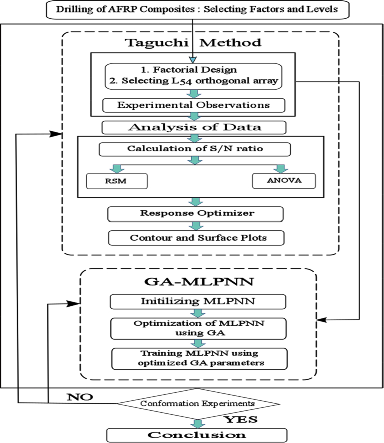
For the GA operation population size of 20, and mutation and crossover, the rate of 0.2 and 0.6 were selected. This optimum weight and bias were embedded into 4-5-1 existing MLPNN as new weight and bias. Optimum values of thrust and torque values were chosen by training the MLPNN network. MLPNN-GA process is shown in Fig. 6 and optimization flowchart is shown in Fig. 7.

Fig. 6.

Structure of MLPNN-GA.

Fig. 7.

Flowchart for optimization.

3.5. Response optimizer (RO)

Response optimizer is one of the tools of RSM. In this work, RO was used to find the optimum parameters for the thrust and torque force. It is an advanced tool to optimize the set of response variables by a combination of input variables. It quantifies the relationship between the controllable input parameters and the obtained response surfaces. It calculates the optimal solution, produces an optimization plot and performs the sensitivity analysis.

4. Results and discussion

This section is divided into four subsections: (1) Hypothesis, (2) Analysis of RSM, MLPNN-GA, and ANOVA predictive mode, (3) Effect of process parameters on thrust and torque force, and (4) Selection of optimum parameters.

4.1. Hypothesis

The following assumptions were made for analyzing the thrust and torque models:

• •The loading of the tool is uniformly distributed and not present at the centre of tool;
• •The laminate does not bend during drilling under the thrust or torque generated by the tool; and
• •Peel up delamination was considered negligible as compared to push out delamination.

4.2. Thrust force

The thrust force was measured experimentally and predicted by RSM and MLPNN-GA during the drilling of AFRP composites, as shown in Table 7. In this study, solid carbide drill bit was used.

Table 7.

Experimental and predicted results of thrust force during drilling of AFRP composites.

Test no.	THRUST				Test no.	THRUST
	aExp.	RSM	bMLPNN	cMLPNN-GA		aExp.	RSM	bMLPNN	cMLPNN-GA
1	98.32	98.928	97.243	100.923	28	122.31	123.919	123.134	123.684
2	100.61	100.957	101.342	99.266	29	126.76	126.465	124.327	127.138
3	101.45	102.027	103.221	101.022	30	129.44	128.052	130.579	129.421
4	87.59	88.097	88.812	87.398	31	120.04	113.186	118.254	119.791
5	91.75	91.387	91.403	90.839	32	113.78	116.993	115.610	113.003
6	94.49	93.717	92.720	95.676	33	118.49	119.840	119.090	118.881
7	74.68	77.716	75.322	73.542	34	102.06	102.903	103.902	102.767
8	86.03	82.267	87.625	87.355	35	104.72	107.971	106.192	103.059
9	86.77	85.858	86.420	85.635	36	113.07	112.079	111.119	113.280
10	112.44	111.498	110.532	110.238	37	137.37	137.617	138.193	138.358
11	114.43	112.412	113.309	113.022	38	137.72	139.048	136.763	138.132
12	111.52	112.366	110.238	112.079	39	138.87	139.519	138.391	137.206
13	98.57	100.590	99.601	99.841	40	128.59	126.807	127.924	127.773
14	102.92	102.765	103.758	101.261	41	130.06	129.499	131.014	129.658
15	102.40	103.980	101.005	103.813	42	132.54	131.230	130.605	133.815
16	91.84	90.132	92.142	91.104	43	114.84	116.447	113.065	114.945
17	93.50	93.568	93.351	91.738	44	121.71	120.399	123.520	119.578
18	94.26	96.043	94.461	95.735	45	123.73	123.392	124.220	124.637
19	107.55	108.265	108.091	108.971	46	134.29	135.512	132.781	135.257
20	108.32	108.064	106.635	108.270	47	135.65	135.827	134.133	135.376
21	109.03	106.902	107.503	110.901	48	136.48	135.183	134.187	136.417
22	98.45	97.280	100.034	98.967	49	125.43	124.624	126.897	125.127
23	96.28	98.339	97.320	96.315	50	126.62	126.201	127.011	126.337
24	97.64	98.439	98.912	98.944	51	124.15	126.817	125.773	124.389
25	87.94	86.745	88.154	87.903	52	112.14	114.187	113.264	113.290
26	88.72	89.065	89.987	88.188	53	118.67	117.024	117.442	119.439
27	90.33	90.425	91.468	90.443	54	120.11	118.901	123.001	121.024
					Error (Avg.)		1.23%	1.100%	0.83%

^aExperimental.

^bAverage values for 54 trials of MLPNN-initial weights and bias.

^cAverage values for 54 trials of MLPNN after optimizing the initial weights and bias using MLPNN-GA model.

4.2.1. Analysis of predictive models

4.2.1.1. Analysis of ANOVA

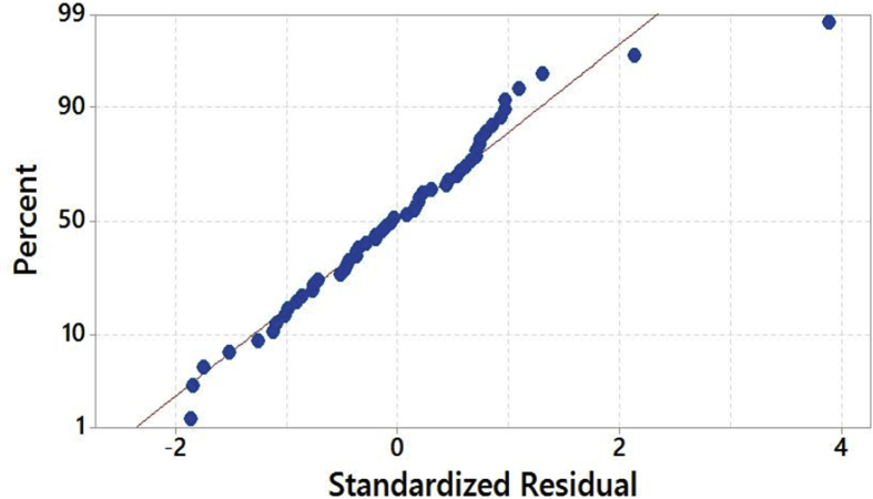
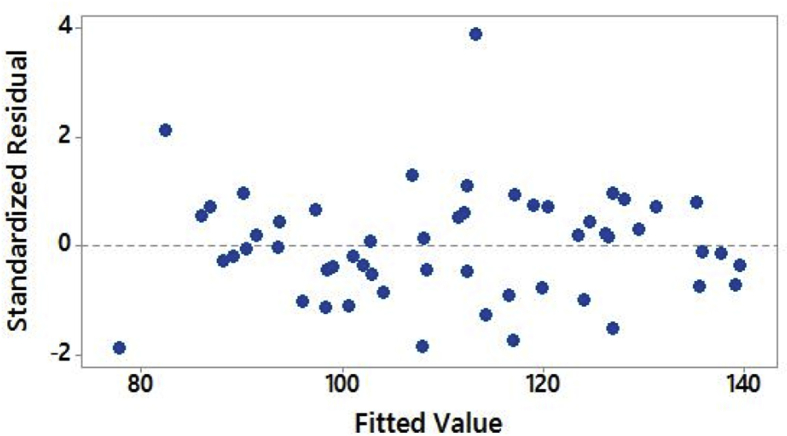
The goodness of the fit ANOVA had been performed and the results of ANOVA are shown in Table 8. The P-values less than 0.05 indicated that the model was quite adequate at 95% confidence limit. In addition, the goodness of the fit had been tested by the correlation coefficient, R². The predicted R² value of 97.93% is in good agreement with an adjusted R² value of 98.50%. So, it confirmed that the model could be accepted; and the values DA, DD, speed, and feed were directly related to thrust force. However, DA and speed were the most significant factors affecting the thrust force. Moreover, residual analysis was performed to check the accuracy of the model. The normal probability plot of the residuals of thrust force is shown in Figs. 8 and 9 illustrates that the errors were normally distributed and follow a straight line which supported the least square fit. The value of R² is found to be 98.87% indicating an excellent goodness of the fit and clarified that excellent variation in the output between response and targets.

Table 8.

Analysis of Variance (ANOVA) for thrust force.

Source	DF	Seq SS	Adj SS	Adj MS	F-value	P-value	% Contribution
Model	13	14370.9	14370.9	1105.45	268.53	0.000	98.87%
Linear	4	13536.2	13536.2	3384.05	822.04	0.000	93.12%
DA	1	9648.3	9648.3	9648.33	2343.73	0.000	66.38%
DD	1	587.6	587.6	587.58	142.73	0.000	4.04%
SPEED	1	3162.9	3162.9	3162.94	768.33	0.000	21.76%
FEED	1	137.4	137.4	137.36	33.37	0.000	0.94%
Square	3	752.6	752.6	250.87	60.94	0.000	5.18%
DD*DD	1	749.2	749.2	749.24	182.00	0.000	5.15%
SPEED*SPEED	1	0.6	0.6	0.61	0.15	0.703	0.00%
FEED*FEED	1	2.8	2.8	2.76	0.67	0.417	0.02%
2-Way interaction	6	82.1	82.1	13.68	3.32	0.009	0.56%
DA*DD	1	11.4	11.4	11.45	2.78	0.103	0.08%
DA*SPEED	1	0.1	0.1	0.09	0.02	0.886	0.00%
DA*FEED	1	2.4	2.4	2.40	0.58	0.449	0.02%
DD*SPEED	1	0.1	0.1	0.14	0.03	0.853	0.00%
DD*FEED	1	29.9	29.9	29.86	7.25	0.010	0.21%
SPEED*FEED	1	38.2	38.2	38.15	9.27	0.004	0.26%
Error	40	164.7	164.7	4.12			1.13%
Total	53	14535.6					100.00%
Model summary of ANOVA			S	R-sq	R-sq(adj)	R-sq(pred)
			2.02896	98.87%	98.50%	97.93%

R-sq = R²; Percentage variation with respect to the response. Higher the R² value, better is the model fitness.

R-sq(adj) = adjusted R²; Percentage variation with respect to the response. Value is adjusted relative to number of predictors and observations in the model. It helps in choosing the correct model by number of predictors.

R-sq(pred) = predicted R²; It determines how well the model predicts when observation is removed.

Fig. 8.

Normal probability plot of residuals.

Fig. 9.

Plot of residuals against fitted values.

Equation (9) describes the calculated thrust force from regression coefficients of Equation (5).

THRUST = −85.1 + 0.728 DA + 33.32 DD − 0.0485 SPEED + 0.144 FEED − 1.975 DD*DD + 0.000002 SPEED*SPEED − 0.000768 FEED*FEED + 0.0201 DA*DD + 0.000012 DA*SPEED + 0.000738 DA*FEED − 0.000128 DD*SPEED − 0.02231 DD*FEED + 0.000168 SPEED*FEED (9)

4.2.1.2. Analysis of MLPNN-GA

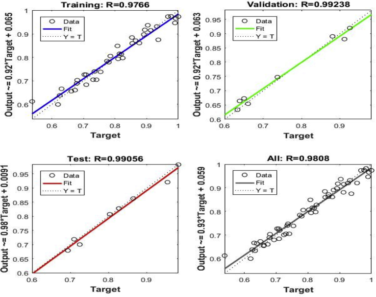
Fig. 10 shows linear regression between training, validation, and testing of MLPNN-GA model after optimizing the initial weight and bias of MLPNN model. From Fig. 10, it is confirmed that target line ratio of MLPNN-GA model oscillated slightly demonstrating that the predicted value differed from experimentally measured value. Moreover, the predicted values were nearer to one which signified that there is an excellent linear relationship between the output value and experimentally determined value. The optimal MLPNN-GA configuration obtained is 4-5-1 (five neurons in N_h) with learning rate and momentum rate values of 0.7534 and 0.0025 respectively. Final values of MLPNN training record are shown in Table 9.

Fig. 10.

Linear regressions of predictions and targets of MLPNN-GA thrust force.

Table 9.

MLPNN training record for thrust force.

Parameter	Value
trainFcn	‘traingdx’
trainParam	[1 × 1 nnetParam]
performFcn	‘mse’
performParam	[1 × 1 struct]
derivFcn	‘defaultderiv’
divideFcn	‘dividerand’
divideMode	‘sample’
divideParam	[1 × 1 struct]
trainInd	[1 × 38 double]
valInd	[2 3 12 18 33 36 44 53]
testInd	[11 13 27 29 31 41 43 48]
stop	‘Maximum epoch reached.’
num_epochs	5000
trainMask	{[1 × 54 double]}
valMask	{[1 × 54 double]}
testMask	{[1 × 54 double]}
best_epoch	18
goal	0
states	{‘epoch’ ‘time’ ‘perf’ ‘vperf’ ‘tperf’ ‘gradient’ ‘val_fail’ ‘lr’}
epoch	[1 × 5001 double]
time	[1 × 5001 double]
perf	[1 × 5001 double]
vperf	[1 × 5001 double]
tperf	[1 × 5001 double]
gradient	[1 × 5001 double]
val_fail	[1 × 5001 double]
lr	[1 × 5001 double]
best_perf	5.5930
best_vperf	0.3192
best_tperf	4.0740

4.2.1.3. Comparison of RSM, MLPNN and MLPNN-GA models

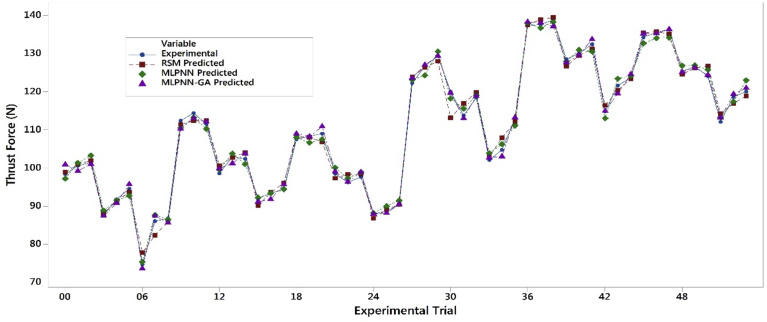
Table 7 and Fig. 11 exhibited the values and plots of experimentally measured thrust force and predicted from RSM, MLPNN, and MLPNN-GA. From Table 7 and Fig. 11, it is observed that MLPNN-GA model exhibited lower variations than the MLPNN model and MLPNN model was bound to local minima [37]. From Fig. 11, it is confirmed that RSM and MLPNN-GA predicted values were closely related to experimentally measured thrust force. Before optimization of initial weights and bias, an average error of 1.1% was noticed with MLPNN. However, when weights and biases were optimized using MLPNN-GA model, the average error was reduced to 0.83% and the number of times required to train MLPNN-GA also reduced. The study showed that MLPNN-GA has less average error than that of RSM. Though, RSM and MLPNN-GA models achieved an average error of less than 4%, and both the models could be used for predicting thrust force during drilling of AFRP composites. From the Table 7, we can realize that average error of RSM was greater than MLPNN and GA-MLPNN techniques. The reason could be due to RSM is a straightforward approach and there no place for tuning the values. On the other hand, in MLPNN-GA the fine-tuning of the weight and bias of MLPNN could be done; and new weight and bias can be re-uploaded to the existing neural network to get the final accurate and precision values. From Fig. 10 its confirmed that MLPNN-GA model has superior performance and computation time taken by MLPNN-GA was 20 times more than that of RSM.

Fig. 11.

Comparison of experiment and predicted results for thrust force.

4.2.2. Effect of process parameters on thrust force

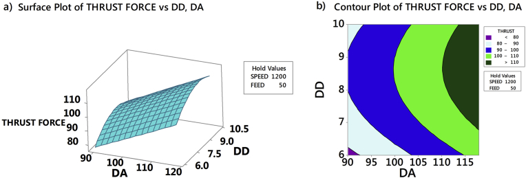
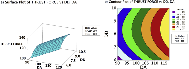
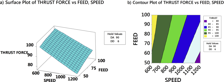
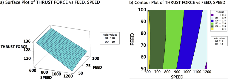
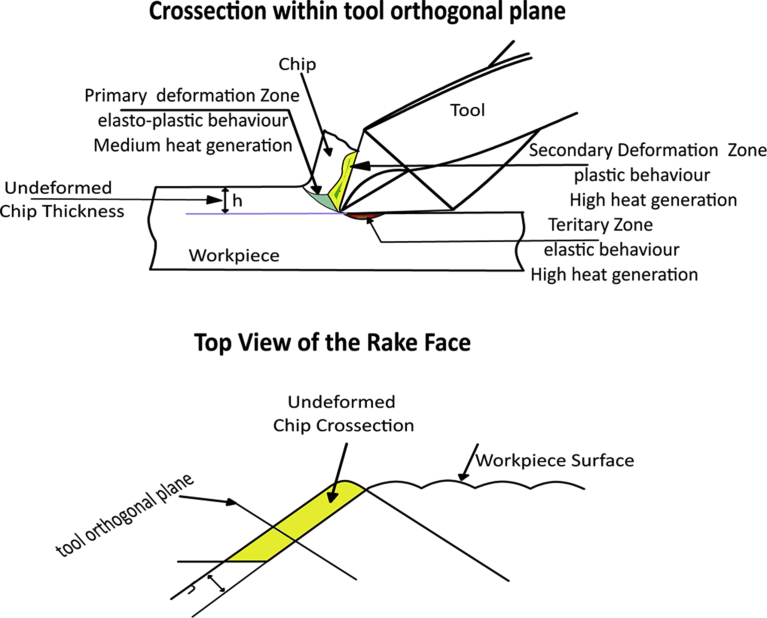
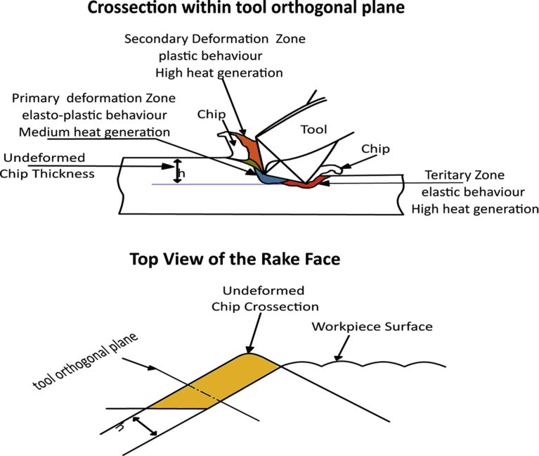
Thrust force in the drilling of AFRP composites had been analyzed through RSM by generating 3D response surface plots and counterplots. Fig. 12a and b exhibits the influence of drill point angle and drill diameter on thrust force when speed and feed was held constant at 1200 rpm and 50 mm/min respectively. Fig. 13a and b exhibits the effect of drill point angle and drill diameter on thrust force when speed and feed was held constant at 600 rpm and 100 mm/min respectively. From Figs. 12a and 13a, observed that drill point angle and drill diameter were sensitive to thrust force and non-linear to the given speed and feed. Similarly, at higher speed and lower feed the induced thrust force was less than that of the lower speed and higher feed, see Figs. 12b and 13b. The study showed that irrespective of the drill point angle and drill diameter, higher speed and lower feed was necessary to obtain less thrust force; which justified the importance of high-speed in drilling [10, 15]. Fig. 14a and b exhibited the interaction of SPEED and FEED on thrust force when drill point angle and drill diameter held constant at 90° and 6 mm respectively. Similarly, interaction due to SPEED and FEED on thrust force, when drill point angle and feed was held constant at 118° and 10 mm respectively is highlighted in Fig. 15a and b. From Figs. 14a and 15a confirmed that speed and feed vary linearly with the chosen drill point angle and drill diameter; and from Figs. 14b and 15b observed that maintaining lower drill point angle and drill diameter resulted in less thrust force. Thus, overall study results indicated that minimum thrust force resulted from the combination of lower values of drill point angle, drill diameter, feed, and higher amounts of speed. Also, from response surface analysis, it is confirmed that low values of drill point angle and drill diameter is advantageous in the drilling of AFRP composites to reduce the damage. However, rise in cutting speed resulted in temperature increase due to friction between the board and the cutting edge, which led to softening of the matrix. This resulted in decrease of cut fibres and less deformed matrix, hence lower damage to the surface. When the drill point angle is reduced, the cross-sectional area of un-deformed chip decreased which resulted in cutting edge angle reduction. Hence, the thrust force is reduced as shown in Figs. 16 and 17. Moreover when the drill diameter was increased, the contact area of the hole also augmented which resulted in increased thrust force. Similarly, the feed rate is in direct relationship with the area of cut; as the feed increased the area of cut increased which demanded more thrust force and caused damage to the workpiece.

Fig. 12.

Effect of drill point angle and drill diameter on thrust force for a speed = 1200 rpm and feed = 50 mm/min.

Fig. 13.

Effect of drill point angle and drill diameter on thrust force for a speed = 600 rpm and feed = 100 mm/min.

Fig. 14.

Effect of speed and feed on thrust force for a point angle = 90° and drill diameter = 6 mm.

Fig. 15.

Effect of speed and feed on thrust force for a point angle = 118° and drill diameter = 10 mm.

Fig. 16.

Drill point angle 90°.

Fig. 17.

Drill point angle 118°.

4.2.3. Selection of optimum parameters

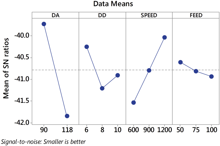
The obtained thrust force results were transformed into S-N ratio using Equation (9). Table 10 and Fig. 18 represent response table for S-N ratio and plot of S-N ratio respectively. Delta values measure the size of the effect by taking the difference between the highest and least characteristic average for a factor. From Table 10 and Fig. 18, it is confirmed that drill point angle is the most significant factor affecting the thrust force followed by spindle speed, drill diameter and feed.

Table 10.

Response table for signal to noise ratios.

Level	DA	DD	SPEED	FEED
1	−39.72	−40.25	−41.53	−40.60
2	−41.85	−41.21	−40.79	−40.82
3		−40.90	−40.03	−40.93
Delta	2.12	0.96	1.50	0.33
Rank	1	3	2	4

Fig. 18.

Thrust force: plot of S-N ratio.

4.2.4. Optimization of thrust force

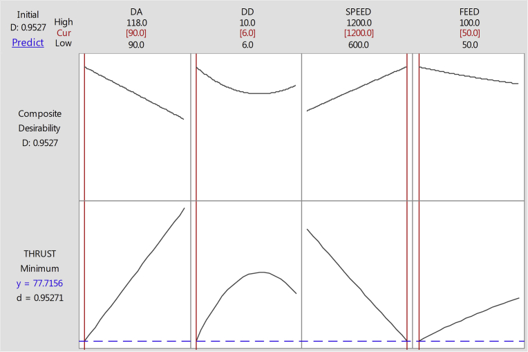
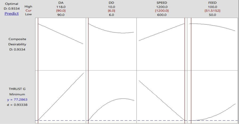
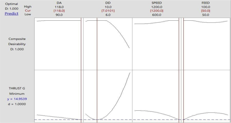
RSM and MLPNN-GA were used to optimize the torque force. From Figs. 19 and 20 confirmed that optimal values of thrust force were close to each other with a deviation of less than 1% error. Thus, from the study it is confirmed that both RSM and MLPNN-GA could be used for modeling the thrust force. According to Figs. 19 and 20 the DA value of 90°, DD of 6 mm, the speed of 1200 rpm and feed of 50 mm/min is the best combination to obtain the minimum thrust force.

Fig. 19.

RSM: optimization plot of thrust force.

Fig. 20.

MLPNN-GA: optimization plot of thrust force.

4.3. Torque

Table 11 represents the experimentally measured toque force using solid carbide drill bit and predicted from RSM and MLPNN-GA.

Table 11.

Experimental and predicted results of torque force during drilling of AFRP composite.

Test no.	TORQUE				Test no.	TORQUE
	Exp.	RSM	MLPNN	MLPNN-GA		Exp.	RSM	MLPNN	MLPNN-GA
1	20.82	19.989	20.664	20.141	28	18.33	17.983	17.297	18.038
2	20.64	20.114	20.331	19.691	29	16.66	18.039	16.277	17.133
3	20.24	19.488	20.229	20.905	30	16.16	17.344	16.007	16.392
4	17.41	18.295	17.013	17.429	31	17.02	17.161	17.061	17.040
5	18.20	18.701	18.321	19.126	32	17.80	17.498	16.566	17.408
6	18.03	18.354	18.961	18.643	33	17.83	17.082	17.340	18.046
7	15.99	15.805	15.397	15.570	34	15.59	15.542	15.912	16.010
8	16.79	16.490	16.219	16.993	35	16.51	16.159	16.022	16.605
9	16.91	16.424	16.187	17.086	36	15.57	16.023	16.211	15.570
10	22.09	20.005	23.129	21.907	37	17.30	17.644	17.757	17.047
11	20.01	20.282	20.315	20.239	38	17.75	17.852	18.882	17.628
12	20.33	19.807	21.091	20.079	39	18.22	17.309	19.008	17.884
13	16.19	18.685	16.802	15.679	40	18.02	17.197	18.305	17.047
14	17.55	19.243	17.493	17.869	41	17.90	17.685	18.533	17.964
15	18.39	19.048	19.331	19.133	42	17.68	17.421	16.723	18.113
16	16.56	16.569	17.222	16.584	43	16.19	15.952	16.099	17.048
17	17.41	17.406	16.129	17.708	44	17.26	16.720	17.434	17.219
18	17.28	17.491	17.595	17.899	45	16.93	16.736	17.883	16.500
19	25.39	26.578	25.934	25.853	46	23.62	23.863	23.447	23.752
20	26.14	27.007	26.127	26.211	47	24.80	24.223	24.002	24.923
21	25.75	26.684	25.574	25.577	48	23.80	23.831	23.893	25.111
22	26.68	25.633	28.113	26.472	49	23.89	23.790	23.400	23.203
23	27.80	26.342	27.404	27.556	50	24.86	24.430	25.601	24.553
24	27.45	26.299	28.371	26.076	51	24.49	24.318	24.254	24.709
25	24.43	23.891	25.421	24.354	52	21.99	22.919	22.633	22.697
26	25.72	24.880	26.822	26.330	53	23.12	23.839	23.766	22.931
27	24.44	25.117	25.413	24.942	54	23.29	24.007	22.040	22.995
					Error (Avg.)		3.09%	2.950%	1.960%

4.3.1. Analysis of RSM, MLPNN-GA and ANOVA predictive models

4.3.1.1. Analysis of RSM

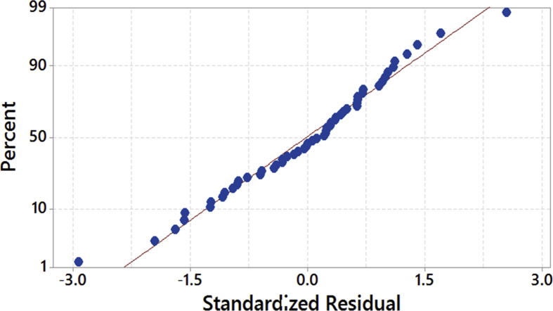
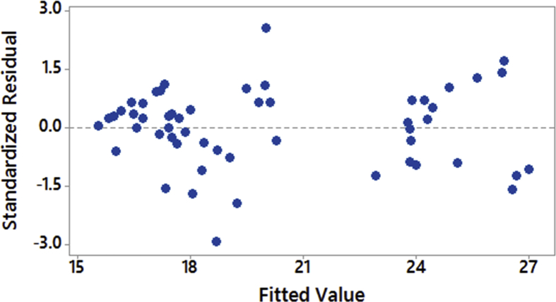
The goodness of the fit ANOVA had been performed, and the results of ANOVA are shown in Table 12. The P-values less than 0.05 indicated that the model is quite adequate at 95% confidence limit. Further, the goodness of the fit had been tested by the correlation coefficient, R². The predicted R² value of 91.33% is in good agreement with adjusted R² value of 93.57% and confirmed that the model could be accepted. The studies proved that DA and speed were the most significant factors affecting torque. Residual analysis was performed to check the accuracy of the model. The normal probability plot of the residuals of torque is shown in Figs. 21 and 22. The study results illustrated that errors were normally distributed and follow a straight-line path. The value of R² is found to be 95.14% and proper variation between the response and targets. Equation (10) explains the calculated thrust force from regression coefficients obtained from Equation (5).

TORQUE = 70.24–0.0910 DA − 11.42 DD − 0.01395 SPEED + 0.0485 FEED + 0.8197 DD*DD − 0.000004 SPEED*SPEED − 0.000602 FEED*FEED − 0.00633 DA*DD + 0.000104 DA*SPEED − 0.000098 DA*FEED + 0.000624 DD*SPEED + 0.00303 DD*FEED + 0.000037 SPEED*FEED (10)

Table 12.

Analysis of variance (ANOVA) for torque.

Source	DF	Seq SS	Adj SS	Adj MS	F-value	P-value	% Contribution
Model	13	693.957	693.957	53.381	95.14%	95.14%	95.14%
Linear	4	547.534	547.534	136.884	75.07%	75.07%	75.07%
DA	1	32.760	32.760	32.760	4.49%	4.49%	4.49%
DD	1	477.860	477.860	477.860	65.52%-	65.52%	65.52%
SPEED	1	36.140	36.140	36.140	4.95%	4.95%	4.95%
FEED	1	0.774	0.774	0.774	0.11%	0.11%	0.11%
Square	3	132.618	132.618	44.206	18.18%	18.18%	18.18%
DD*DD	1	129.013	129.013	129.01	17.69%	17.69%	17.69%
SPEED*SPEED	1	1.907	1.907	1.907	0.26%	0.26%	0.26%
FEED*FEED	1	1.698	1.698	1.698	0.23%	0.23%	0.23%
2-Way interaction	6	13.805	13.80	2.30	1.89%	1.89%	1.89%
DA*DD	1	1.131	1.131	1.131	0.16%	0.16%	0.16%
DA*SPEED	1	6.838	6.838	6.838	0.94%	0.94%	0.94%
DA*FEED	1	0.043	0.043	0.043	0.01%	0.01%	0.01%
DD*SPEED	1	3.360	3.360	3.360	0.46%	0.46%	0.46%
DD*FEED	1	0.552	0.552	0.552	0.08%	0.08%	0.08%
SPEED*FEED	1	1.882	1.882	1.882	0.26%	0.26%	0.26%
Error	40	35.412	35.412	0.885	4.86%	4.86%	4.86%
Total	53	729.369			100.00%	100.00%	100.00%
Model summary of ANOVA		S		R-sq	R-sq (adj)	R-sq (pred)
		0.940904		95.14%	93.57%	91.33%

Fig. 21.

Normal probability plot of residuals.

Fig. 22.

Residuals versus fitted values.

4.3.1.2. Analysis of MLPNN-GA

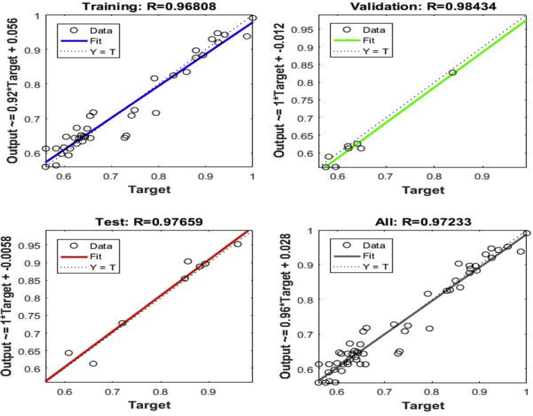
The linear regression between training, validation, and testing of MLPNN-GA model is shown in Fig. 23. From Fig. 23 it is confirmed that the target line ratio of MLPNN-GA model oscillated slightly; indicating that the predicted value differed from the experimentally measured value. The predicted values were nearer to one which means that there is a good linear relationship between the output value and experimentally measured value. The obtained optimal MLPNN-GA configuration is 4-5-1 (five neurons in N_h) with learning rate and momentum rate as 0.8512 and 0.0027 respectively. Final values of MLPNN training record are shown in Table 13.

Fig. 23.

Linear regressions of predictions and targets of MLPNN-GA.

Table 13.

MLPNN training record for torque force.

Parameter	Value
trainFcn	‘traingdx’
trainParam	[1 × 1 nnetParam]
performFcn	‘mse’
performParam	[1 × 1 struct]
derivFcn	‘defaultderiv’
divideFcn	‘dividerand’
divideMode	‘sample’
divideParam	[1 × 1 struct]
trainInd	[1 × 38 double]
valInd	[3 6 8 12 27 47 48 50]
testInd	[4 15 18 20 30 41 43 51]
stop	‘Maximum epoch reached.’
num_epochs	5000
trainMask	{[1 × 54 double]}
valMask	{[1 × 54 double]}
testMask	{[1 × 54 double]}
best_epoch	96
goal	0
states	{‘epoch’ ‘time’ ‘perf’ ‘vperf’ ‘tperf’ ‘gradient’ ‘val_fail’ ‘lr’}
epoch	[1 × 5001 double]
time	[1 × 5001 double]
perf	[1 × 5001 double]
vperf	[1 × 5001 double]
tperf	[1 × 5001 double]
gradient	[1 × 5001 double]
val_fail	[1 × 5001 double]
lr	[1 × 5001 double]
best_perf	0.3858
best_vperf	1.4342
best_tperf	0.6894

4.3.1.3. Comparison of RSM, MLPNN-GA and ANOVA predictive models

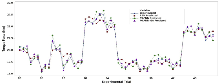
Table 11 and Fig. 24 shows the comparison of experimentally measured torque force and values predicted by RSM, MLPNN, and MLPNN-GA respectively. It was observed that MLPNN-GA model exhibited lower variations than the MLPNN model. From Fig. 24, observed that RSM and MLPNN-GA predicted values were closely related to experimentally measured torque force. Furthermore, from Table 11 confirmed that an average error of 2.95% with MLPNN was observed before optimization of initial weights and bias. When weights and biases were optimized using MLPNN-GA model, the average error was reduced to 1.60% and the number of times required training the MLPNN-GA also significantly reduced. The study results indicated that both RSM and MLPNN-GA models achieved an average error less than 4%, and both the models could be used for predicting the torque while drilling of AFRP composites. From Fig. 23 it can be confirmed that MLPNN-GA model has excellent performance and computation time taken by MLPNN-GA is 25 times more than that of RSM.

Fig. 24.

Comparison plots of experimental and predicted results.

4.3.2. Influence of process parameters on torque

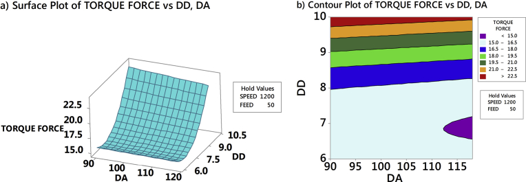
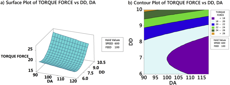
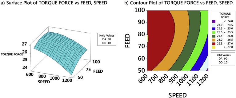
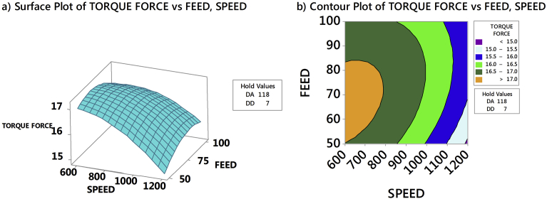
Torque in the drilling of AFRP composites had been analyzed through RSM predicted model by generating 3D response surface plots and counterplots. Fig. 25a and b exhibits the effect of drill point angle and drill diameter on torque with speed and feed held constant at 1200 rpm and 50 mm/min respectively. Fig. 26a and b exhibits effect of drill point angle and drill diameter on torque with speed and feed held constant at 600 rpm and 100 mm/min respectively. From Figs. 25a and 26a, perceived that drill point angle and drill diameter were sensitive to torque force and linear to the given speed and feed. From the study, it was confirmed that torque is much lesser at drill diameter of 7 mm. Figs. 25b and 26b confirmed that the induced torque was lower at higher speed and lower feed. This indicated that irrespective of drill point angle and drill diameter, higher speed and lower feed is necessary to obtain lower torque. Fig. 27a and b emphasized the effect of SPEED and FEED on torque with drill point angle and drill diameter held constant at 90° and 10 mm respectively. Similarly, Fig. 28a and b highlighted the effect of SPEED and FEED on torque with drill point angle and feed held constant at 118° and 7 mm respectively. From Figs. 27a and 28a, confirmed that speed and feed vary non-linearly with drill point angle and drill diameter. Also, from Figs. 27b and 28b observed that maintaining a higher drill point angle and lower drill diameter resulted in less torque. Thus, from the study it is confirmed that minimum torque resulted from combination of lower values of drill diameter and feed, and higher values of speed and drill point angle, which is necessary in the drilling of AFRP composites. As the cutting speed increased there is an increase in temperature due to friction between the board and the cutting edge. This led to softening of the matrix which resulted in less amount of material gets attached to the drill bit and less deterioration of the drilling surface. Also, at larger drill point angle, the tool has small lip length which created the less torque. Similarly, the contact area of the hole enlarged with increase in the drill diameter, which resulted rise in the torque. Furthermore, the feed rate is in direct relationship with specific cutting energy. The area of specific cutting energy also increased with enhanced feed, which demanded high torque and more damage to AFRP composites.

Fig. 25.

Effect of drill point angle and drill diameter on torque for a speed = 1200 rpm and feed = 50 mm/min.

Fig. 26.

Effect of drill point angle and drill diameter on torque for a speed = 600 rpm and feed = 100 mm/min.

Fig. 27.

Effect of speed and feed on torque for a point angle = 90° and drill diameter = 10 mm.

Fig. 28.

Effect of speed and feed on torque for a point angle = 118° and drill diameter = 7 mm.

4.3.3. Selection of optimum parameters

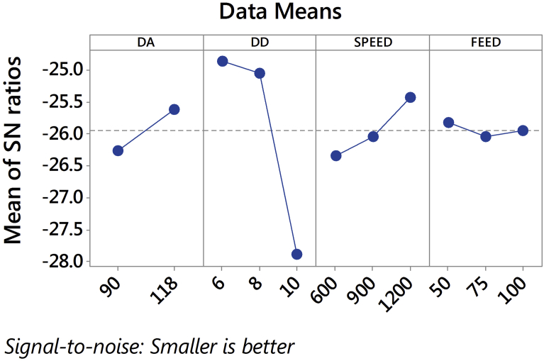
The obtained torque results were transformed into S-N ratio using Equation (10). Table 14 and Fig. 29 represent the response table for S-N ratio and plot of S-N ratio respectively. From the Table 12 delta values and Fig. 29, it is clear that drill diameter, drill point angle are the most significant factors affecting the torque. These results were in line with surface and counterplots of torque.

Table 14.

Response table for signal to noise ratios.

Level	DA	DD	SPEED	FEED
1	−26.26	−24.87	−26.35	−25.82
2	−25.62	−25.05	−26.04	−26.05
3		−27.90	−25.44	−25.95
Delta	0.64	3.03	0.91	0.23
Rank	3	1	2	4

Fig. 29.

Torque force: plot of S-N ratio.

4.3.4. Optimization of torque force

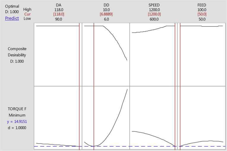
RSM and MLPNN-GA were used to optimize the torque force and plots were generated using 'MINITAB′ software. Figs. 30 and 31 plots showed the optimum combinations of the factors were required to achieve the minimum torque force. It can be seen that optimal values of torque were close to each other with a deviation of less than 1%. The study results demarcated that both RSM and MLPNN-GA could be used for modeling of torque force. According to Figs. 30 and 31, DA value of 118°, DD of 7 mm, Speed of 1200 rpm and feed of 50 mm/min are the best combination to obtain the minimum torque.

Fig. 30.

RSM: optimization plot of torque.

Fig. 31.

MLPNN-GA: optimization plot of torque.

5. Conclusions

An investigative analysis of the influence of process parameters on thrust force and torque in the drilling of Aramid Fibre Reinforced Plastic (AFRP) composites had been carried out in this paper and the following are the outcomes of the work:

• 1.The thrust force and torque were studied with respect to cutting speed, feed rate, drill point angle and drill diameter by developing RSM and MLPNN-GA models. The developed MLPNN-GA model provided higher accuracy than RSM. The predicted values of thrust force and torque of RSM and MLPNN-GA models closely matched with the experimental values which signified the accuracy of the developed model.
• 2.The values of optimum thrust force and torque were obtained by response optimizer of RSM and MLPNN-GA. They were close to each other with a deviation of less than 1% error. This showed that MLPNN-GA model could be used effectively to predict drilling parameters in AFRP composites.
• 3.The study indicated that parameters required to obtain the minimum thrust force are 90°drill point angle, 6 mm drill diameter, 1200 rpm spindle speed and 50 mm/min feed rate. Similarly, parameters to obtain the minimum torque force are 118° drill point angle, 6.9 ∼ 7 mm drill diameter, 1200 rpm spindle speed and 50 mm/min feed rate.
• 4.This study recommends the use of high speed and low feed combination and drill point angles of 90°–118° to reduce the delamination of the materials in the drilling of AFRP composites. Also, normal probability plots of the residuals follow a straight-line pattern indicating that this work would be useful for industries during the selection of process parameters for drilling of AFRP composites.

Declarations

Author contribution statement

Anarghya A., Harshith D.N., Nitish Rao: Analyzed and interpreted the data; Contributed reagents, materials, analysis tools or data; Wrote the paper.

Nagaraj S. Nayak: Conceived and designed the experiments; Analyzed and interpreted the data; Contributed reagents, materials, analysis tools or data.

Gurumurthy B.M., Abhishek V.N., Ishwar Gouda S. Patil: Performed the experiments; Analyzed and interpreted the data; Contributed reagents, materials, analysis tools or data; Wrote the paper.

Funding statement

This research did not receive any specific grant from funding agencies in the public, commercial, or not-for-profit sectors.

Competing interest statement

The authors declare no conflict of interest.

Additional information

No additional information is available for this paper.

References

- 1.Soutis C. Fibre reinforced composites in aircraft construction. Prog. Aerosp. Sci. 2005;41:143–151. [Google Scholar]
- 2.Singh T.J., Samanta S. Characterization of Kevlar fibre and its composites: a review. Mater. Today Proc. 2015;2:1381–1387. [Google Scholar]
- 3.Fink J.K. 2014. 13 Aramids; pp. 301–320. [Google Scholar]
- 4.Bishop G.R., Gindy N.N.Z. An investigation into the drilling of ballistic Kevlar composites. Compos. Manuf. 1990;1:155–159. [Google Scholar]
- 5.Zheng L., Zhou H., Gao C., Yuan J. Hole drilling in ceramics/Kevlar fibre reinforced plastics double-plate composite armor using diamond core drill. Mater. Des. 2012;40:461–466. [Google Scholar]
- 6.Di Ilio A., Tagliaferri V., Veniali F. Cutting mechanisms in drilling of aramid composites. Int. J. Mach. Tools Manuf. 1991;31:155–165. [Google Scholar]
- 7.Bhattacharyya D., Horrigan D.P.W. A study of hole drilling. Compos. Sci. Technol. 1998;58:267–283. [Google Scholar]
- 8.Hirogaki T., Aoyama E., Inoue H., Ogawa K., Maeda S., Katayama T. Laser drilling of blind via holes in aramid and glass/epoxy composites for multi-layer printed wiring boards. Compos. Part A Appl. Sci. Manuf. 2001;32:963–968. [Google Scholar]
- 9.Liu D., Tang Y., Cong W.L. A review of mechanical drilling for composite laminates. Compos. Struct. 2012;94:1265–1279. [Google Scholar]
- 10.Feito N., Diaz-Álvarez J., López-Puente J., Miguelez M.H. Numerical analysis of the influence of tool wear and special cutting geometry when drilling woven CFRPs. Compos. Struct. 2016;138:285–294. [Google Scholar]
- 11.Karpat Y., Deger B., Bahtiyar O. Drilling thick fabric woven CFRP laminates with double point angle drills. J. Mater. Process. Technol. 2012;212:2117–2127. [Google Scholar]
- 12.Palanikumar K. Experimental investigation and optimisation in drilling of GFRP composites. Meas. J. Int. Meas. Confed. 2011;44:2138–2148. [Google Scholar]
- 13.sunny T., Babu J., Philip J. Experimental studies on effect of process parameters on delamination in drilling GFRP composites using Taguchi method. Proc. Mater. Sci. 2014;6:1131–1142. [Google Scholar]
- 14.Krishnaraj V., Prabukarthi A., Ramanathan A., Elanghovan N., Kumar M.S., Zitoune R., Davim J.P. Composites: part B optimization of machining parameters at high speed drilling of carbon fibre reinforced plastic (CFRP) laminates. Compos. Part B. 2012;43:1791–1799. [Google Scholar]
- 15.Mohan N.S., Ramachandra A., Kulkarni S.M. Influence of process parameters on cutting force and torque during drilling of glass-fibre polyester reinforced composites. Compos. Struct. 2005;71:407–413. [Google Scholar]
- 16.Tsao C.C., Hocheng H. Taguchi analysis of delamination associated with various drill bits in drilling of composite material. Int. J. Mach. Tools Manuf. 2004;44:1085–1090. [Google Scholar]
- 17.Tsao C.C., Chiu Y.C. Evaluation of drilling parameters on thrust force in drilling carbon fibre reinforced plastic (CFRP) composite laminates using compound core-special drills. Int. J. Mach. Tools Manuf. 2011;51:740–744. [Google Scholar]
- 18.Khashaba U.A., Selmy A.I., Megahed A.A. Composites: part A machinability analysis in drilling woven GFR/epoxy composites: part I – effect of machining parameters. Compos. Part A Appl. Sci. Manuf. 2010;41:391–400. [Google Scholar]
- 19.Rajamurugan T.V., Shanmugam K., Palanikumar K. Analysis of delamination in drilling glass fibre reinforced polyester composites. Mater. Des. 2013;45:80–87. [Google Scholar]
- 20.Zarif N., Heidary H., Minak G., Ahmadi M. Effect of the drilling process on the compression behavior of glass/epoxy laminates. Compos. Struct. 2013;98:59–68. [Google Scholar]
- 21.Kilickap E. Optimization of cutting parameters on delamination based on Taguchi method during drilling of GFRP composite. Expert Syst. Appl. 2010;37:6116–6122. [Google Scholar]
- 22.Karnik S.R., Gaitonde V.N., Rubio J.C., Correia A.E., Abrão A.M., Davim J.P. Delamination analysis in high speed drilling of carbon fibre reinforced plastics (CFRP) using artificial neural network model. Mater. Des. 2008;29:1768–1776. [Google Scholar]
- 23.Kumar V., Ganta V. Optimization of process parameters in drilling of GFRP composite using Taguchi method. Integr. Med. Res. 2013;3:35–41. [Google Scholar]
- 24.Gaitonde V.N., Karnik S.R., Rubio J.C., Correia A.E., Abrão A.M., Davim J.P. Analysis of parametric influence on delamination in high-speed drilling of carbon fibre reinforced plastic composites. J. Mater. Process. Technol. 2008;203:431–438. [Google Scholar]
- 25.Wang X., Kwon P.Y., Sturtevant C., Kim D.D.W., Lantrip J. Tool wear of coated drills in drilling CFRP. J. Manuf. Process. 2013;15:87–95. [Google Scholar]
- 26.Tsao C.C., Hocheng H., Chen Y.C. Delamination reduction in drilling composite materials by active backup force. CIRP Ann. Manuf. Technol. 2012;61:91–94. [Google Scholar]
- 27.Zarif Karimi N., Heidary H., Minak G. Critical thrust and feed prediction models in drilling of composite laminates. Compos. Struct. 2016;148:19–26. [Google Scholar]
- 28.Rahme P., Landon Y., Lachaud F., Piquet R., Lagarrigue P. Delamination-free drilling of thick composite materials. Compos. Part A Appl. Sci. Manuf. 2015;72:148–159. [Google Scholar]
- 29.Feito N., López-puente J., Santiuste C., Miguélez M.H. Numerical prediction of delamination in CFRP drilling. Compos. Struct. 2014;108:677–683. [Google Scholar]
- 30.Tsao C.C. Experimental study of drilling composite materials with step-core drill. Mater. Des. 2008;29:1740–1744. [Google Scholar]
- 31.Jain A.K., Mao J., Mohiuddin K.M. Artificial neural networks: a tutorial. Comput. Long Beach Calif. 1996;29:31–44. [Google Scholar]
- 32.a Shahin M., Jaksa M.B., Maier H.R. Artificial neural network applications in geotechnical engineering. Aust. Geomech. 2001;36:49–62. [Google Scholar]
- 33.Haykin S., Networks N., Foundation A.C. Exploring the diversity of artificial neural network architectures. J. Math. Psychol. 1997;292:287–292. [Google Scholar]
- 34.Yegnanarayana B. Prentice-Hall of India; 1999. Artificial Neural Networks.https://books.google.co.in/books/about/ARTIFICIAL_NEURAL_NETWORKS.html?id=RTtvUVU_xL4C [Google Scholar]
- 35.Fogel D.B. Review of computational intelligence: imitating life [Book reviews] Proc. IEEE. 1995;83:1588–1592. [Google Scholar]
- 36.Dini G. Online prediction of delamination in drilling of GFRP by using a neural network approach. Mach. Sci. Technol. 2007 [Google Scholar]
- 37.Enemuoh E.U., El-gizawy A.S., Okafor A.C. An approach for development of damage-free drilling of carbon fibre reinforced thermosets. Int. J. Mach. Tools Manuf. 2001;41:1795–1814. [Google Scholar]
- 38.Yan F., Lin Z. New strategy for anchorage reliability assessment of GFRP bars to concrete using hybrid artificial neural network with genetic algorithm. Compos. Part B. 2016;92:420–433. [Google Scholar]
- 39.Saravanana R.R.M., Ramalingamb D., Manikandanc G. Multi objective optimization of drilling parameters using genetic algorithm. Proc. Eng. 2012;38:197–207. [Google Scholar]
- 40.Krishnaraj V., Prabukarthi A., Ramanathan A., Elanghovan N., Kumar M.S., Zitoune R., Davim J.P. Optimization of machining parameters at high speed drilling of carbon fibre reinforced plastic (CFRP) laminates. Compos. Part B Eng. 2012;43:1791–1799. [Google Scholar]