In silico prediction of chemical subcellular localization via multi-classification methods

Multi-classification models were developed for prediction of subcellular localization of small molecules by machine learning methods.

Abstract

Chemical subcellular localization is closely related to drug distribution in the body and hence important in drug discovery and design. Although many in vivo and in vitro methods have been developed, in silico methods play key roles in the prediction of chemical subcellular localization due to their low costs and high performance. For that purpose, machine learning-based methods were developed here. At first, 614 unique compounds localized in the lysosome, mitochondria, nucleus and plasma membrane were collected from the literature. 80% of the compounds were used to build the models and the rest as the external validation set. Both fingerprints and molecular descriptors were used to describe the molecules, and six machine learning methods were applied to build the multi-classification models. The performance of the models was measured by 5-fold cross-validation and external validation. We further detected key substructures for each localization and analyzed potential structure–localization relationships, which could be very helpful for molecular design and modification. The key substructures can also be used as features complementary to fingerprints to improve the performance of the models.

Introduction

In human cells, drug targets are usually located in different subcellular organelles, such as nuclei and mitochondria. Since subcellular organelles have different functions and microenvironments, drugs tend to distribute in these subcellular organelles with different concentrations, which determines the amount of drugs binding to the targets. Therefore, it is very important to understand the distribution of drugs at a subcellular level during drug discovery. Meanwhile, a compound that accumulates in wrong organelles may increase its toxicity.1

The distribution of compounds at the subcellular level is usually examined by experimental approaches. However, in vivo and in vitro approaches are very complicated, expensive and time-consuming, and in silico methods are hence widely used in prediction of chemical properties due to their advantages such as speed, low cost and accuracy. Currently, there are a lot of studies focusing on in silico prediction of the subcellular localization of proteins, to reveal their functions and the primary machinery of the cell, which are critical to further understanding the intricate pathways at the cellular level.2–4 Nevertheless, in silico studies on the subcellular localization of small molecules were very few. The subcellular localization of small molecules usually depends on their physicochemical properties and thus chemical structures. Therefore, based on chemical structures, in silico prediction of chemical subcellular localization would be practicable and helpful for molecular design and reduction of potential toxicity.

The in silico prediction methods for subcellular localization can be primarily divided into statistics-based regression and mechanism-based physiological ones. These two types of methods are complementary.5 The latter are more convincing and explicable but complicated enough to construct widely applicable models. There is some excellent work on simulating the diffusion and transportation of compounds in cells.6–8 As for the statistics-based models, most studies concentrate on the relationships between physicochemical or structural descriptors and chemical concentrations in a specific subcellular organelle.9–12 Although in those models, physicochemical properties such as log P and molecular weight are adequate, these properties may not be suitable to distinguish at the subcellular level. As studied by Zheng et al., the physicochemical properties (molecular weight, log P, formal charge, dipole moment, globularity, number of H-bond donors and rotatable bond fraction) could not well distinguish the subcellular distribution of compounds.13 So it is urgent to develop new methods to predict chemical subcellular localization accurately.

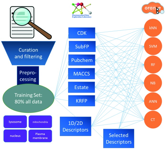
In this study, we developed statistics-based multi-classification models to predict chemical subcellular localization utilizing machine learning algorithms. The multi-classification models have been successfully applied in toxicity prediction in our previous work.14,15 Both molecular descriptors and fingerprints were considered as features, while key substructures were detected and added as new features to improve the predictive models further. According to the data we collected, four locations were chosen to construct the models, namely the lysosome, mitochondria, nucleus, and plasma membrane. As pointed out in a comprehensive review,16 more and more topics in life sciences actually belong to the multi-label system. For example, the same protein may occur in two and more than two subcellular location sites. Researchers tend to build multi-label models for the prediction of the subcellular localization of proteins.17–22 However, due to the limitation of the data we collected, only one subcellular location was considered for each compound here. We will try to develop multi-label models for chemical subcellular localization when more reliable data are available.

As demonstrated by a series of recent publications23–26 in complying with the 5-step rule,27 to establish a really useful statistical predictor for a biological or biomedical system, we need to consider the following procedures: (a) construct a valid benchmark dataset to train and test the predictor; (b) formulate the compounds with an effective mathematical expression that can truly reflect their intrinsic correlation with the target to be predicted; (c) develop a powerful method to operate the prediction; (d) properly perform cross-validation tests to objectively evaluate the anticipated accuracy of the predictor; (e) provide a user-friendly and publicly accessible web server for the predictor. As shown below, let us describe how to deal with these steps one by one.

Methods

Data collection and preparation

All data were collected from four sources.9,10,12,28 For compounds that only had names or CI (color index) numbers available, their chemical structures were obtained by manual search from DrugBank,29 ChemNet (; chemnet.com) and others. Duplicates, ambivalent and multi-localized compounds were removed. Compounds localized in the ER/Golgi and cytosol were also removed because their numbers were not enough to be considered in this study.

The data set was then prepared through the following steps: (1) removing mixtures, inorganic salts and organometallic compounds; (2) removing compounds with molecular weights less than 40 or more than 800; (3) converting compounds into canonical SMILES through Open Babel.30

80% of the compounds were used as the training set to build the predictive models. The rest (20%) served as the external validation set to evaluate the capability and accuracy of the models.

Calculation of molecular descriptors and fingerprints

In order to construct multi-classification models, 1444 1D/2D molecular descriptors were calculated by PaDEL-Descriptor,31 including physicochemical, topological and electronic properties. Six fingerprints were also generated by PaDEL-Descriptor, including MACCS32 (166 bits from MDL public keys), SubFP (also called FP4 in Open Babel, 307 bits), CDK (designed by Chemistry Development Kit,33 1024 bits), Estate (designed by Hall et al.,34 79 bits), KRFP (designed by Klekota et al.,35 4860 bits), and Pubchem (designed by PubChem,36 881 bits). The MACCS fingerprint was also used to calculate the Tanimoto similarity of the data set.

Feature selection

Each fingerprint type was directly used as a feature set to build models without any feature selection. After the key substructures were identified later, the key substructures were also added into the six types of fingerprints as new feature sets. The new feature sets were named by adding a suffix “+” after the corresponding fingerprint name. For example, MACCS contains 166 bits of features representing the property or fragment of compounds, while “MACCS+” contains not only the 166 bits of primary features but also the key substructures mined by SARpy.

For molecular descriptors, the features that could not be calculated for all the compounds were removed. Then, three feature selection methods were employed on the molecular descriptors to avoid overfitting.20

Decision tree

When building a decision tree, the attribute with the highest normalized IG value was chosen as a node at the first level and the data were separated into two sets after the decision. For each set, a new node would be built as the second level. Then, the tree was built until a threshold is reached to prevent overfitting. All the nodes in the final tree were considered as important features.

F-score

F-score is a simple technique which measures the discrimination of two sets of real numbers. It was firstly designed to improve the performance of support vector machines for binary classification.37 In this study, we used an improved F-score, which was extended from the original one, shown in eqn (1).

1

In this equation, “i” means the ith feature, “j” means the subcellular location, and “k” means the kth compound (located in the j location).

Greedy stepwise

This is a forward stepwise feature selection method that considers all the molecular descriptors and picks the best one to be correlated with the localization.38 WEKA,39 a free JAVA package, was employed and the evaluator function of the method is the “CfssubsetEval” set in WEKA.

Model building

Six machine learning methods were employed to build the models, namely support vector machine40 (SVM), C4.5 decision tree41 (CT), random forest42 (RF), k-nearest neighbor43 (kNN), naïve Bayes44 (NB), and artificial neural network45 (ANN). These methods were performed using Orange46 (version 2.7.8, ; http://orange.biolab.si/orange2/).

SVM was originally designed to be implemented in binary classification. To implement SVM in multi-classification, several extended approaches were developed and compared.47 Our previous study demonstrated that the OAO (one against one) method performed better than the others,14 so OAO was used here for multi-classification of SVMs. The parameters of SVM (C and gamma) were optimized through a python script in the LIBSVM package.48 In the kNN, ANN and RF models, the parameters (k in kNN, number of nodes in the hidden layer in ANN and number of trees in RF) were optimized by scanning.

Assessment of model performance

5-fold cross-validation was implemented to evaluate the performance of the models in order to discard the improper algorithms and descriptors. At the same time, we could compare the performance of molecular descriptors with the fingerprints. All the models were then evaluated using the external validation set.

The models were assessed by the counts of true positives (TP) of each class. The predictive accuracy (Q_i) of each class and the total predictive accuracy (Q) were calculated by using the following equations:

2

3

Here, P_i means the number of compounds localizing in the ith subcellular organelle and P means all compounds.

Identification of key substructures

SARpy49 was employed to detect key substructures that emerge frequently in a specific subcellular organelle. SARpy is a free standalone and easy-to-use tool which uses “string mining” to directly generate substructures from the SMILES notation and uses “likelihood ratio” to evaluate the significance of each substructure. The equation of likelihood is shown below.

4

For each subcellular organelle, localized compounds were marked as positive, and the others were tagged as negative. TP, true positive, means the number of compounds which contain the substructure and are localized in the subcellular organelle. FP, false positive, means the number of compounds which contain the substructure but are not localized in it. P and N respectively represent the number of “positive” compounds and “negative” compounds. The parameter we used in SARpy was “OPTIMAL” in the extraction of key substructures.

To further refine the key substructures and extract knowledge for molecular design, Open Babel and its python API, Pybel,50 were used to calculate the frequency of each substructure in the data set. Apart from the likelihood calculated by SARpy, we employed another two indices to evaluate the importance of a substructure, i.e. accuracy (ACC) and information gain (IG). ACC is the ratio between the number of true positive compounds and the number of total compounds containing the substructure. The algorithm and application of IG were introduced in our previous work.51 It should be noted that the data set was divided into four classes and the key substructures were analyzed for each location separately.

Results

Dataset analysis

The training set and external validation set contained 491 and 123 compounds, respectively, which were localized in four subcellular organelles, namely the lysosome, mitochondria, nucleus, and plasma membrane, as shown in Table 1. The majority of the compounds are drugs, dyes and their analogs.

Table 1. Number of compounds in the data set divided by localization.

Localization	Training set	Validation set	Total
Endo-lysosomes	132	32	164
Mitochondria	190	46	236
Nucleus	81	22	103
Plasma membrane	88	23	111
Total	491	123	614

To investigate the distribution of each class of compounds in the chemical space, six physicochemical properties of the compounds were calculated by Discovery Studio 3.5,52 which were A log P, molecular weight (MW), log D, log S, and the numbers of H-bond donors (HBD) and acceptors (HBA). The principal component analysis (PCA) was employed to scatter them into a 2D diagram, presented in Fig. 1A. The PCA result showed that the physicochemical properties of compounds targeting different subcellular organelles were similar and could not diverge from each other. In addition, the chemical space of a set of 1006 FDA-approved small molecular drugs (MW ≤800) from DrugBank was compared with the training set. As shown in Fig. 1B, the external validation set shared a similar chemical space with the training set, which covered most of the approved drugs. The drugs that could not be covered were saccharides, whose numbers of H-bond donors and acceptors are high, compounds containing phosphorus, sulfur or other atom types, and inorganic drugs. The training set contained a lot of dyes which are different from drugs, and its chemical space was more diverse. The average similarity of the whole data set was 0.321, and most of the similarities were distributed in 0.1 to 0.5 (Fig. 2A). The similarity matrix (shown in Fig. 2B) illustrated that the compounds in our data set were generally diverse. The compounds were ordered by their localization as lysosome, mitochondria, nucleus, and plasma membrane. The hot fields were mainly located in no. 300–500 and around 600, which were compounds localized in the plasma membrane.

Fig. 1. Chemical space defined by the two principal components from six physicochemical properties. A) Training set data in the chemical space colored by subcellular localization: orange for lysosome, pink for mitochondria, green for nucleus, and violet for plasma membrane. B) All data distribution in the chemical space: red for the training set, green for the external validation set, and black for the FDA-approved drugs with molecular weight <800.

Fig. 2. A) Distribution of molecular similarity calculated with the MACCS fingerprint and Tanimoto coefficient. B) Similarity matrix of the compounds, in which 0 (blue) means the least similarity and 1 (red) means the highest similarity (but does not mean that they are the same).

Selected molecular descriptors and fingerprints

After removing the descriptors that could not be calculated for all compounds by PaDEL-Descriptor, 1380 ones were kept. A decision tree was constructed with the default parameters in Orange and 38 features emerged in the tree. According to the construction of the decision tree, compounds with ETA_dEpsilon_D < 0.015 were primarily localized in the mitochondria and plasma membrane, while others were mainly localized in the lysosome, mitochondria and nucleus. Compounds with ETA_dEpsilon_D > 0.015 and MLFER_BO < 1.165 were primarily localized in the lysosome. ETA_dEpsilon_D53 is used to measure the contribution of hydrogen-bond donor atoms, and MLFER_BO54 is the overall or summation solute (octanol or ethyl acetate as solvents) hydrogen bond basicity.

Meanwhile, the greedy stepwise method automatically gave the finally optimized features without presetting other parameters and 78 features were selected. By F-score, topoDiameter and topoRadius were the top two features and Crippen log P and X log P were respectively ranked in 7 and 8, indicating that topological and physicochemical properties were important in classification. According to the F-score values, the top 20 and top 100 features were selected to build the models, respectively.

Furthermore, SARpy obtained 46 key substructures in total from the training set, 6 for the lysosome, 20 for mitochondria, 9 for the nucleus, and 11 for the plasma membrane. These substructures were matched to the compounds in the training set. If the substructure occurs in a compound, the compound labels 1 as the feature. All the 46 features were added to each of the six fingerprints as prior knowledge to improve the models further.

Performance of multi-classification models in cross-validation

At first, 66 machine learning-based models were built, which used six machine learning methods with eleven types of molecular description, i.e. MACCS, CDK, SubFP, Estate, Pubchem, KRFP, full 1D/2D descriptors (Full_Des), and four descriptor sets with feature selection. Meanwhile, 5-fold cross-validation was implemented to evaluate the performance of the models. As shown in Table 2, the results illustrated that the greedy stepwise and decision tree selection methods performed better than F-score. The best total accuracy was 71.5% by decision tree selected features with the ANN method. The performance of outstanding models is presented in Table 3 (full results are shown in Table S1‡ and Fig. 3). Among these models, the MACCS-SVM model performed the best, whose prediction accuracies were 72.0% for the lysosome, 81.1% for mitochondria, 67.9% for the nucleus, and 79.5% for the plasma membrane, respectively. The total accuracy of the MACCS-SVM model was 76.2%. By using all molecular descriptors, competitive performance could be reached. The Full_Des-SVM one performed the best. The predictive accuracies were respectively 72.9%, 82.3%, 65.4%, and 77.3% for the four subcellular organelles, and the total accuracy was 76.1%. Other models such as CDK-SVM, CDK-ANN, Pubchem-SVM, and KRFP-SVM also performed well, whose total accuracies were respectively 75.6%, 74.7%, 74.5%, and 75.3%. From the general view of the results (Fig. 3), SVM could reach the highest accuracy with both fingerprints and 1D/2D descriptors. kNN performed better with 1D/2D descriptors than that with fingerprints. CT and NB performed the worst and might not be suitable for prediction in this system. Though the models with full descriptors performed well compared to the models with fingerprints and selected features, it is less acceptable due to their too many descriptors considering the limited training samples.

Table 2. The performance of selected features by total predictive accuracy.

	kNN	SVM	NB	RF	ANN	CT
Full_Des	0.755	0.761	0.609	0.660	0.731	0.573
Greedy stepwise	0.705	0.672	0.646	0.662	0.712	0.580
F-score 20	0.637	0.495	0.430	0.687	0.640	0.576
F-score 100	0.566	0.493	0.448	0.635	0.686	0.614
Decision tree	0.700	0.613	0.599	0.581	0.715	0.617

Table 3. Performance of outstanding models from 5-fold cross-validation.

Model name	Q total	Q 1	Q 2	Q 3	Q 4
MACCS-SVM	0.762	0.720	0.811	0.679	0.795
Full_Des-SVM	0.761	0.729	0.823	0.654	0.773
CDK-SVM	0.756	0.705	0.811	0.728	0.739
Full_Des-kNN	0.755	0.699	0.750	0.765	0.841
KRFP-SVM	0.753	0.674	0.832	0.679	0.773
CDK-ANN	0.747	0.720	0.753	0.765	0.761
Pubchem-SVM	0.745	0.727	0.763	0.691	0.784
Full_Des-ANN	0.731	0.707	0.776	0.667	0.727
MACCS-RF	0.727	0.682	0.832	0.580	0.705
KRFP-ANN	0.725	0.697	0.726	0.667	0.818

Fig. 3. The performance of the models in cross-validation.

External validation of models

Compounds in the validation set did not participate in feature selection and model construction to ensure the reliability. The detailed results of the models are illustrated in Table 4. From an overview of the results, the performance of all the models was better than that from cross-validation. In general, the best models in cross-validation also kept the best performance in external validation. The Full_Des-SVM model performed the best compared to the models using fingerprints as features. The accuracies for the different locations were 87.9%, 91.3%, 77.3%, and 69.6%, respectively. The MACCS-SVM, CDK-SVM and CDK-ANN models were still in the top positions.

Table 4. Performance of excellent models in the external validation set compared with the performance in cross-validation.

Model name	Q total	Q 1	Q 2	Q 3	Q 4
MACCS-SVM	0.772	0.812	0.848	0.682	0.772
Full_Des-SVM	0.839	0.879	0.913	0.773	0.696
CDK-SVM	0.821	0.812	0.935	0.773	0.652
Full_Des-kNN	0.790	0.758	0.848	0.727	0.783
KRFP-SVM	0.813	0.812	0.870	0.773	0.739
CDK-ANN	0.764	0.812	0.826	0.682	0.652
Pubchem-SVM	0.797	0.812	0.891	0.727	0.652
Full_Des-ANN	0.726	0.697	0.826	0.682	0.607
MACCS-RF	0.756	0.750	0.891	0.500	0.739
KRFP-ANN	0.805	0.781	0.891	0.773	0.696

In addition, the fingerprints with added key substructures were compared with the primary fingerprints. Fig. 4 illustrates the performance of the models with original fingerprints and original fingerprints plus key substructures mined by SARpy below. From an overview, most models performed better with the additional features, especially Estate and SubFP. KRFP with additional features could reach the highest accuracy, which is 83.7% in the external validation set. The results indicate that with key substructures as new features added to fingerprints, the performance of classification models can be improved.

Fig. 4. Comparison between fingerprints (fingerprint) and fingerprints with added key substructures (fingerprint+).

Identification of key substructures from all data

A total of 58 substructures were identified key to the subcellular localization from all the datasets by SARpy, which included the 46 substructures mined from the training set. To refine the key substructures, we reserved the substructures with IG >0.02 and accuracy ≥0.7. Finally, 20 key substructures were detected as listed in Table 5 (2 localized in the lysosome, 5 localized in mitochondria, 7 localized in the nucleus, and 6 localized in the plasma membrane). Though some substructures were not significant due to their too low frequency, we should not neglect the fact that substructures with accuracy = 1 still deserved attention. Therefore, we listed the substructures with ACC = 1 and “efficacious frequency” ≥3, which are presented in Table 6. If two or more compounds were very similar visually, the efficacious frequency was only recorded as one. The 2D structures of the significant substructures were drawn by SMARTSviewer,55 as listed in Fig. S2.‡

Table 5. Key substructures with ACC >0.7 and IG >0.02.

No.	Label	Substructure	TP	P	ACC	IG
1	Lysosome		36	50	0.72	0.057
2	Lysosome		9	9	1	0.028
3	Mitochondria		12	12	1	0.027
4	Mitochondria		10	10	1	0.022
5	Mitochondria		17	18	0.94	0.031
6	Mitochondria		12	13	0.92	0.02
7	Mitochondria		17	20	0.85	0.02
8	Nucleus		14	14	1	0.06
9	Nucleus		6	6	1	0.025
10	Nucleus		5	5	1	0.021
11	Nucleus		5	5	1	0.021
12	Nucleus		11	13	0.86	0.035
13	Nucleus		12	15	0.8	0.027
14	Nucleus		10	13	0.77	0.027
15	Plasma membrane		40	40	1	0.176
16	Plasma membrane		22	22	1	0.093
17	Plasma membrane		8	8	1	0.032
18	Plasma membrane		20	20	1	0.083
19	Plasma membrane		24	24	1	0.102
20	Plasma membrane		19	20	0.95	0.071

Table 6. Substructures with ACC = 1 but IG <0.02.

No.	Localization	Substructure	TP	P	ACC	IG
21	Lysosome		3	3	1	0.0092
22	Mitochondria		6	6	1	0.0134
23	Mitochondria		5	5	1	0.0112
24	Mitochondria		3	3	1	0.0067
25	Plasma membrane		4	4	1	0.0162

Discussion

Relationships of physicochemical properties with subcellular localization

Molecular weight, log P and other physicochemical properties affect the absorption, distribution, metabolism and excretion (ADME) of compounds in the human body. In drug discovery, these physicochemical properties dictate whether a compound is drug-like and guide the modification of a lead compound. Some QSAR models use molecular weight, log P or other common physicochemical properties to build chemical space, while others directly use these properties to build models. Considering that the six physicochemical properties (MW, A log P, log D, log S, HBD, HBA) are important in drug discovery and highly relevant to the characteristics of compounds in cells and organs, we used these descriptors to build the chemical space, and compared the compounds with drugs in a PCA scatter diagram to evaluate the diversity.

It is a key factor to select suitable features to describe chemicals when building prediction models. But at the subcellular level, the physicochemical properties contributed little to the preference of the localization of compounds, according to the PCA results. Zheng et al. used linear discriminant analysis with the six properties and obtained similar results.13 So we could say that though common properties could dictate the permeation of compounds into cells, they contribute little to the concentration rate in subcellular organelles. Thus, we calculated more 1D/2D descriptors and fingerprints to build models, considering the structural features of compounds.

Significance of key substructures to subcellular localization and drug design

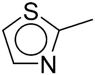
Compared to molecular descriptors and physicochemical properties, the key substructures are more helpful for lead optimization. If one understands the pharmacological mechanism of a medical therapy, adding these specific substructures may improve the distribution of a molecule at the subcellular level, which will further affect the drug efficacy. Some of the key substructures we mined are known functional groups by which researchers could design probes or drugs. For example, triphenylphosphine (TTP), which can accumulate selectively in mitochondria because of its positive charge and lipophilicity, is used in mitochondria-targeted cancer therapy.56,57 Hematoporphyrin derivative (HPD) can be used in mitochondria-targeted photodynamic therapy because of its strong fluorescence and selective localization.58 These two functional groups respectively contained the two key substructures we mined (substructures 4 and 5 in Table 5).

For drugs whose mechanisms are not clear, prediction of their subcellular localization is helpful to exploit their potential targets and pathways. However, the credibility of these key substructures is highly dependent on the quantity and quality (e.g. the diversity of the data set and reliability of the experimental results) of the data used to build the models. We should notice that key substructures are not classifiers; hence, a compound containing a lysosome-substructure could not guarantee that it should be localized in the lysosome.

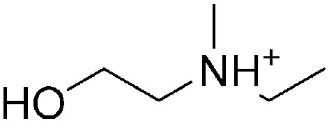
Though computational approaches could help to mine substructures appearing more frequently in one location than the others, it is necessary to deeply analyze key substructures and the corresponding compounds to offset the deficiency of data and methods. Here, we listed two key substructures, 2-hydroxyethan-1-aminium derivatives (1) and N-ethyl-2-hydroxy-N-methylethan-1-aminium derivatives (2), that prefer to be in the lysosome (listed in Table 5). The two substructures have a relationship of inclusion. The bigger one (2) is more specific with a higher likelihood and the smaller one (1) is more common. The positive compounds (which are localized in the lysosome, listed in Table S2‡) are diverse. For most of them, substructure 1 is the main functional group. Therefore, we reported that substructure 1 should be an important functional group to make compounds that prefer to be in the lysosome. Meanwhile, we should also pay attention to the negative compounds which contain the substructure listed in Table S2.‡ Although there are 14 negative compounds, the number of efficient compounds is only 6 because many compounds are analogs and are localized in the same subcellular organelle. Besides, most of these negative compounds are complicated, containing other functional groups. This might explain why the compounds are negative and further ensure the significance of substructure 1. As for substructure 2, though the accuracy of the pattern is very high, it is unexplainable due to only a few positive compounds containing such a fragment available.

Performance of the models

In statistical prediction, the following three cross-validation methods are often used to examine a predictor for its effectiveness in practical application: independent dataset test, subsampling or K-fold cross-validation test, and jackknife test (leave-one-out test).59 However, of the three test methods, the jackknife test is deemed the least arbitrary that can always yield a unique result for a given benchmark dataset.27 Accordingly, the jackknife test has been widely recognized and increasingly used by investigators to examine the quality of various predictors.23–26,60–62 However, to reduce the computational time especially in hyper-parameter optimization, we adopted the 5-fold cross-validation and independent dataset test in this study as conducted by many investigators with SVM as the prediction engine.

The results of cross-validation and external validation showed that the performance of most of the models was reliable, which might be very helpful for us to understand the chemical distribution inside the cell. Though the performance of full molecular descriptors was competitive against molecular fingerprints to describe the chemicals, we still highly recommend using fingerprints to build models. Fingerprints are interpretable, efficient and less redundant, indicating less probability of overfitting.

However, the accuracy of the models remains to be improved, compared to other endpoints in similar studies such as acute oral toxicity14 and carcinogenicity63 we reported previously. Two factors might affect the performance of the models. 1) The quantity of the dataset is not large enough, and the diversity is still to be improved especially for the plasma membrane. The similarity matrix (Fig. 2B) illustrated that the compounds in the plasma membrane were similar in structure, which may narrow the application domain of the models and bias the model towards other localizations. This can explain why the predictive accuracy of the plasma membrane in cross-validation was high compared to the accuracy in external validation (Tables 3 and 4). 2) The process of localization of small molecules inside the cell is complicated. In reality, compounds might be multi-localized inside the cell. To simplify the models, we only considered four major subcellular organelles and mono-localized compounds in this study.

As shown in a series of recent publications,61,62,64–70 user-friendly and publicly accessible web servers will significantly enhance the impacts of predictive models.71 For this purpose, we have added the MACCS-SVM model into our web server admetSAR,72 particularly developed for the prediction of chemical pharmacokinetic properties (freely available at ; http://lmmd.ecust.edu.cn:8000/). Users can predict chemical subcellular localization using the model in the “predict” page by inputting SMILES of the query molecule. We shall make efforts to improve the quality of our web server in the near future.

Conclusions

In this study, multi-classification models were built to predict subcellular localization of small molecules with CT, RF, NB, kNN, ANN and SVM algorithms. 1D/2D descriptors were calculated as features to build models and three feature selection methods were implemented. Six types of fingerprints, MACCS, SubFP, CDK, Estate, Pubchem, and KRFP, were also used as features and compared with the molecular descriptors. Finally, the full-1D/2D descriptors and MACCS were found best to describe the molecules, and SVM and ANN were excellent in performance. Considering the quality of 1D/2D molecular descriptors and the overfitting risk, we recommend substructure-based fingerprints to build predictive models. Substructure extraction was performed to detect the key substructures that frequently occurred in compounds targeting a specific localization. The key substructures can also be used as new features to improve the classification models. In a nutshell, our study provides a useful multi-classification method to predict the localization of small compounds and we detected significant descriptors and substructures as a kind of knowledge that can guide drug design or molecular modification.

References

- Sancho-Martinez S. M., Prieto-Garcia L., Prieto M., Lopez-Novoa J. M., Lopez-Hernandez F. J. Pharmacol. Ther. 2012;136:35–55. doi: 10.1016/j.pharmthera.2012.07.003. [DOI] [PubMed] [Google Scholar]
- Chou K. C., Shen H. B. Anal. Biochem. 2007;370:1–16. doi: 10.1016/j.ab.2007.07.006. [DOI] [PubMed] [Google Scholar]
- Dehzangi A., Heffernan R., Sharma A., Lyons J., Paliwal K., Sattar A. J. Theor. Biol. 2015;364:284–294. doi: 10.1016/j.jtbi.2014.09.029. [DOI] [PubMed] [Google Scholar]
- Ahmad K., Waris M., Hayat M. J. Membr. Biol. 2016;249:293–304. doi: 10.1007/s00232-015-9868-8. [DOI] [PubMed] [Google Scholar]
- Horobin R. W., Trapp S., Weissig V. J. Controlled Release. 2007;121:125–136. doi: 10.1016/j.jconrel.2007.05.040. [DOI] [PubMed] [Google Scholar]
- Trapp S., Rosania G. R., Horobin R. W., Kornhuber J. Eur. Biophys. J. 2008;37:1317–1328. doi: 10.1007/s00249-008-0338-4. [DOI] [PMC free article] [PubMed] [Google Scholar]
- Baik J., Rosania G. R. J. Pharm. Pharmacol. 2013;1:8. doi: 10.13188/2327-204X.1000004. [DOI] [PMC free article] [PubMed] [Google Scholar]
- Balaz S. Chem. Rev. 2009;109:1793–1899. doi: 10.1021/cr030440j. [DOI] [PMC free article] [PubMed] [Google Scholar]
- Durazo S. A., Kadam R. S., Drechsel D., Patel M., Kompella U. B. Pharm. Res. 2011;28:2833–2847. doi: 10.1007/s11095-011-0532-4. [DOI] [PMC free article] [PubMed] [Google Scholar]
- Colston J., Horobin R. W., Rashid-Doubell F., Pediani J., Johal K. K. Biotech. Histochem. 2003;78:323–332. doi: 10.1080/10520290310001646659. [DOI] [PubMed] [Google Scholar]
- Min K. A., Zhang X., Yu J. Y., Rosania G. R. Biopharm. Drug Dispos. 2014;35:15–32. doi: 10.1002/bdd.1879. [DOI] [PMC free article] [PubMed] [Google Scholar]
- Horobin R. W., Stockert J. C., Rashid-Doubell F. Histochem. Cell Biol. 2006;126:165–175. doi: 10.1007/s00418-006-0156-7. [DOI] [PubMed] [Google Scholar]
- Zheng N., Tsai H. N., Zhang X., Shedden K., Rosania G. R. Mol. Pharmaceutics. 2011;8:1611–1618. doi: 10.1021/mp200093z. [DOI] [PMC free article] [PubMed] [Google Scholar]
- Li X., Chen L., Cheng F., Wu Z., Bian H., Xu C., Li W., Liu G., Shen X., Tang Y. J. Chem. Inf. Model. 2014;54:1061–1069. doi: 10.1021/ci5000467. [DOI] [PubMed] [Google Scholar]
- Li X., Du Z., Wang J., Wu Z., Li W., Liu G., Shen X., Tang Y. Mol. Inf. 2015;34:228–235. doi: 10.1002/minf.201400127. [DOI] [PubMed] [Google Scholar]
- Chou K. C. Mol. BioSyst. 2013;9:1092–1100. doi: 10.1039/c3mb25555g. [DOI] [PubMed] [Google Scholar]
- Chou K. C., Wu Z. C., Xiao X. PLoS One. 2011;6:e18258. doi: 10.1371/journal.pone.0018258. [DOI] [PMC free article] [PubMed] [Google Scholar]
- Wu Z. C., Xiao X., Chou K. C. Mol. BioSyst. 2011;7:3287–3297. doi: 10.1039/c1mb05232b. [DOI] [PubMed] [Google Scholar]
- Xiao X., Wu Z. C., Chou K. C. J. Theor. Biol. 2011;284:42–51. doi: 10.1016/j.jtbi.2011.06.005. [DOI] [PubMed] [Google Scholar]
- Chou K. C., Wu Z. C., Xiao X. Mol. BioSyst. 2012;8:629–641. doi: 10.1039/c1mb05420a. [DOI] [PubMed] [Google Scholar]
- Wu Z. C., Xiao X., Chou K. C. Protein Pept. Lett. 2012;19:4–14. doi: 10.2174/092986612798472839. [DOI] [PubMed] [Google Scholar]
- Lin W. Z., Fang J. A., Xiao X., Chou K. C. Mol. BioSyst. 2013;9:634–644. doi: 10.1039/c3mb25466f. [DOI] [PubMed] [Google Scholar]
- Qiu W. R., Sun B. Q., Xiao X., Xu Z. C., Chou K. C. Bioinformatics. 2016;32:3116–3123. doi: 10.1093/bioinformatics/btw380. [DOI] [PubMed] [Google Scholar]
- Cheng X., Zhao S. G., Xiao X., Chou K. C. Bioinformatics. 2017;33:341–346. doi: 10.1093/bioinformatics/btw644. [DOI] [PubMed] [Google Scholar]
- Khan M., Hayat M., Khan S. A., Iqbal N. J. Theor. Biol. 2017;415:13–19. doi: 10.1016/j.jtbi.2016.12.004. [DOI] [PubMed] [Google Scholar]
- Liu B., Wang S., Long R., Chou K. C. Bioinformatics. 2017;33:35–41. doi: 10.1093/bioinformatics/btw539. [DOI] [PubMed] [Google Scholar]
- Chou K. C. J. Theor. Biol. 2011;273:236–247. doi: 10.1016/j.jtbi.2010.12.024. [DOI] [PMC free article] [PubMed] [Google Scholar]
- Zheng N., Tsai H. N., Zhang X., Rosania G. R. Mol. Pharmaceutics. 2011;8:1619–1628. doi: 10.1021/mp200092v. [DOI] [PMC free article] [PubMed] [Google Scholar]
- Knox C., Law V., Jewison T., Liu P., Ly S., Frolkis A., Pon A., Banco K., Mak C., Neveu V., Djoumbou Y., Eisner R., Guo A. C., Wishart D. S. Nucleic Acids Res. 2011;39:D1035–D1041. doi: 10.1093/nar/gkq1126. [DOI] [PMC free article] [PubMed] [Google Scholar]
- O'Boyle N. M., Banck M., James C. A., Morley C., Vandermeersch T., Hutchison G. R. J. Cheminf. 2011;3:33. doi: 10.1186/1758-2946-3-33. [DOI] [PMC free article] [PubMed] [Google Scholar]
- Yap C. W. J. Comput. Chem. 2011;32:1466–1474. doi: 10.1002/jcc.21707. [DOI] [PubMed] [Google Scholar]
- Durant J. L., Leland B. A., Henry D. R., Nourse J. G. J. Chem. Inf. Comput. Sci. 2002;42:1273–1280. doi: 10.1021/ci010132r. [DOI] [PubMed] [Google Scholar]
- Steinbeck C., Han Y. Q., Kuhn S., Horlacher O., Luttmann E., Willighagen E. J. Chem. Inf. Comput. Sci. 2003;43:493–500. doi: 10.1021/ci025584y. [DOI] [PMC free article] [PubMed] [Google Scholar]
- Hall L. H., Kier L. B. J. Chem. Inf. Model. 1995;35:1039–1045. [Google Scholar]
- Klekota J., Roth F. P. Bioinformatics. 2008;24:2518–2525. doi: 10.1093/bioinformatics/btn479. [DOI] [PMC free article] [PubMed] [Google Scholar]
- PubChem Substructure Fingerprint, ftp://ftp.ncbi.nlm.nih.gov/pubchem/specifications/pubchem_fingerprints.txt.
- Chen Y.-W. and Lin C.-J., in Feature Extraction: Foundations and Applications, ed. I. Guyon, M. Nikravesh, S. Gunn and L. A. Zadeh, Springer Berlin Heidelberg, Berlin, Heidelberg, 2006, pp. 315–324, 10.1007/978-3-540-35488-8_13. [DOI] [Google Scholar]
- Newby D., Freitas A. A., Ghafourian T. J. Chem. Inf. Model. 2013;53:2730–2742. doi: 10.1021/ci400378j. [DOI] [PubMed] [Google Scholar]
- Frank E., Hall M., Trigg L., Holmes G., Witten I. H. Bioinformatics. 2004;20:2479–2481. doi: 10.1093/bioinformatics/bth261. [DOI] [PubMed] [Google Scholar]
- Cortes C., Vapnik V. Mach. Learn. 1995;20:273–297. [Google Scholar]
- Quinlan J. R., C4. 5: programs for machine learning, Elsevier, 2014. [Google Scholar]
- Breiman L. Mach. Learn. 2001;45:5–32. [Google Scholar]
- Cover T., Hart P. IEEE Trans. Inf. Theory. 1967;13:21–27. [Google Scholar]
- Watson P. J. Chem. Inf. Model. 2008;48:166–178. doi: 10.1021/ci7003253. [DOI] [PubMed] [Google Scholar]
- Basheer I. A., Hajmeer M. J. Microbiol. Methods. 2000;43:3–31. doi: 10.1016/s0167-7012(00)00201-3. [DOI] [PubMed] [Google Scholar]
- Demsar J., Curk T., Erjavec A., Gorup C., Hocevar T., Milutinovic M., Mozina M., Polajnar M., Toplak M., Staric A., Stajdohar M., Umek L., Zagar L., Zbontar J., Zitnik M., Zupan B. J. Mach. Learn. Res. 2013;14:2349–2353. [Google Scholar]
- Li H., Qi F. and Wang S., in Computational Science and Its Applications – ICCSA 2005: International Conference, Singapore, May 9-12, 2005, Proceedings, Part IV, ed. O. Gervasi, M. L. Gavrilova, V. Kumar, A. Laganá, H. P. Lee, Y. Mun, D. Taniar and C. J. K. Tan, Springer Berlin Heidelberg, Berlin, Heidelberg, 2005, pp. 1140–1148, 10.1007/11424925_119. [DOI] [Google Scholar]
- Chang C. C., Lin C. J. ACM Trans. Intell. Syst. Technol. 2011;2:1–27. [Google Scholar]
- Ferrari T., Cattaneo D., Gini G., Bakhtyari N. G., Manganaro A., Benfenati E. SAR QSAR Environ. Res. 2013;24:631–649. doi: 10.1080/1062936X.2013.773376. [DOI] [PubMed] [Google Scholar]
- O'Boyle N. M., Morley C., Hutchison G. R. Chem. Cent. J. 2008;2:5. doi: 10.1186/1752-153X-2-5. [DOI] [PMC free article] [PubMed] [Google Scholar]
- Shen J., Cheng F., Xu Y., Li W., Tang Y. J. Chem. Inf. Model. 2010;50:1034–1041. doi: 10.1021/ci100104j. [DOI] [PubMed] [Google Scholar]
- Discovery Studio 3.5, Accelrys, San Diego, CA, 2017.
- Roy K., Das R. N. SAR QSAR Environ. Res. 2011;22:451–472. doi: 10.1080/1062936X.2011.569900. [DOI] [PubMed] [Google Scholar]
- Platts J. A., Butina D., Abraham M. H., Hersey A. J. Chem. Inf. Comput. Sci. 1999;39:835–845. doi: 10.1021/ci990427t. [DOI] [PubMed] [Google Scholar]
- Schomburg K., Ehrlich H. C., Stierand K., Rarey M. J. Chem. Inf. Model. 2010;50:1529–1535. doi: 10.1021/ci100209a. [DOI] [PubMed] [Google Scholar]
- Hu Q., Gao M., Feng G., Liu B. Angew. Chem., Int. Ed. 2014;53:14225–14229. doi: 10.1002/anie.201408897. [DOI] [PubMed] [Google Scholar]
- Kong X., Su F., Zhang L., Yaron J., Lee F., Shi Z., Tian Y., Meldrum D. R. Angew. Chem., Int. Ed. 2015;54:12053–12057. doi: 10.1002/anie.201506038. [DOI] [PMC free article] [PubMed] [Google Scholar]
- Rangasamy S., Ju H., Um S., Oh D. C., Song J. M. J. Med. Chem. 2015;58:6864–6874. doi: 10.1021/acs.jmedchem.5b01095. [DOI] [PubMed] [Google Scholar]
- Chou K. C., Zhang C. T. Crit. Rev. Biochem. Mol. Biol. 1995;30:275–349. doi: 10.3109/10409239509083488. [DOI] [PubMed] [Google Scholar]
- Sharma R., Dehzangi A., Lyons J., Paliwal K., Tsunoda T., Sharma A. IEEE Trans. Nanobioscience. 2015;14:915–926. doi: 10.1109/TNB.2015.2500186. [DOI] [PubMed] [Google Scholar]
- Chen W., Feng P., Yang H., Ding H., Lin H., Chou K. C. Oncotarget. 2017;8:4208–4217. doi: 10.18632/oncotarget.13758. [DOI] [PMC free article] [PubMed] [Google Scholar]
- Meher P. K., Sahu T. K., Saini V., Rao A. R. Sci. Rep. 2017;7:42362. doi: 10.1038/srep42362. [DOI] [PMC free article] [PubMed] [Google Scholar]
- Li X., Du Z., Wang J., Wu Z. R., Li W. H., Liu G. X., Shen X., Tang Y. Mol. Inf. 2015;34:228–235. doi: 10.1002/minf.201400127. [DOI] [PubMed] [Google Scholar]
- Chen W., Ding H., Feng P., Lin H., Chou K. C. Oncotarget. 2016;7:16895–16909. doi: 10.18632/oncotarget.7815. [DOI] [PMC free article] [PubMed] [Google Scholar]
- Jia J., Liu Z., Xiao X., Liu B., Chou K. C. Oncotarget. 2016;7:34558–34570. doi: 10.18632/oncotarget.9148. [DOI] [PMC free article] [PubMed] [Google Scholar]
- Liu B., Wu H., Zhang D. Y., Wang X. L., Chou K. C. Oncotarget. 2017;8:13338–13343. doi: 10.18632/oncotarget.14524. [DOI] [PMC free article] [PubMed] [Google Scholar]
- Qiu W. R., Sun B. Q., Xiao X., Xu Z. C., Chou K. C. Oncotarget. 2016;7:44310–44321. doi: 10.18632/oncotarget.10027. [DOI] [PMC free article] [PubMed] [Google Scholar]
- Qiu W. R., Xiao X., Xu Z. C., Chou K. C. Oncotarget. 2016;7:51270–51283. doi: 10.18632/oncotarget.9987. [DOI] [PMC free article] [PubMed] [Google Scholar]
- Xiao X., Ye H. X., Liu Z., Jia J. H., Chou K. C. Oncotarget. 2016;7:34180–34189. doi: 10.18632/oncotarget.9057. [DOI] [PMC free article] [PubMed] [Google Scholar]
- Zhang C. J., Tang H., Li W. C., Lin H., Chen W., Chou K. C. Oncotarget. 2016;7:69783–69793. doi: 10.18632/oncotarget.11975. [DOI] [PMC free article] [PubMed] [Google Scholar]
- Chou K. C. Med. Chem. 2015;11:218–234. doi: 10.2174/1573406411666141229162834. [DOI] [PubMed] [Google Scholar]
- Cheng F., Li W., Zhou Y., Shen J., Wu Z., Liu G., Lee P. W., Tang Y. J. Chem. Inf. Model. 2012;52:3099–3105. doi: 10.1021/ci300367a. [DOI] [PubMed] [Google Scholar]
Associated Data
This section collects any data citations, data availability statements, or supplementary materials included in this article.