Repeated Measures Designs and Analysis of Longitudinal Data: If at First You Do Not Succeed—Try, Try Again

Abstract

Anesthesia, critical care, perioperative, and pain research often involves study designs in which the same outcome variable is repeatedly measured or observed over time on the same patients. Such repeatedly measured data are referred to as longitudinal data, and longitudinal study designs are commonly used to investigate changes in an outcome over time and to compare these changes among treatment groups. From a statistical perspective, longitudinal studies usually increase the precision of estimated treatment effects, thus increasing the power to detect such effects. Commonly used statistical techniques mostly assume independence of the observations or measurements. However, values repeatedly measured in the same individual will usually be more similar to each other than values of different individuals and ignoring the correlation between repeated measurements may lead to biased estimates as well as invalid P values and confidence intervals. Therefore, appropriate analysis of repeated-measures data requires specific statistical techniques. This tutorial reviews 3 classes of commonly used approaches for the analysis of longitudinal data. The first class uses summary statistics to condense the repeatedly measured information to a single number per subject, thus basically eliminating within-subject repeated measurements and allowing for a straightforward comparison of groups using standard statistical hypothesis tests. The second class is historically popular and comprises the repeated-measures analysis of variance type of analyses. However, strong assumptions that are seldom met in practice and low flexibility limit the usefulness of this approach. The third class comprises modern and flexible regression-based techniques that can be generalized to accommodate a wide range of outcome data including continuous, categorical, and count data. Such methods can be further divided into so-called “population-average statistical models” that focus on the specification of the mean response of the outcome estimated by generalized estimating equations, and “subject-specific models” that allow a full specification of the distribution of the outcome by using random effects to capture within-subject correlations. The choice as to which approach to choose partly depends on the aim of the research and the desired interpretation of the estimated effects (population-average versus subject-specific interpretation). This tutorial discusses aspects of the theoretical background for each technique, and with specific examples of studies published in Anesthesia & Analgesia, demonstrates how these techniques are used in practice.

Repetitio est mater studiorum [Repetition is the mother of learning].

—Latin proverb attributed to the Roman statesman and writer Cassiodorus (circa 485–585)

Medical research often involves study designs in which the same outcome variable is repeatedly observed or measured over time in the same study subjects (patients). Such repeatedly measured data are referred to as longitudinal data. Longitudinal data are typically collected when investigating changes in an outcome variable over time, so as to compare these changes among groups (eg, different treatment groups).^1,2 From a statistical perspective, a longitudinal study usually increases the precision of the estimated treatment effect and increases the power to detect such an effect.^2–4

Many commonly used statistical techniques assume independence of the observations or measurements.⁵ However, values repeatedly measured in the same individual are usually more similar to each other than values from different individuals—and therefore are not independent.⁶ Ignoring this positive correlation between repeated measurements can result in biased estimates, as well as incorrect standard errors of the estimates, resulting in invalid P values and confidence intervals.^7,8

Therefore, appropriate analysis of repeated-measures data requires specific statistical techniques.⁹ As part of the ongoing series in Anesthesia & Analgesia, this tutorial reviews statistical methods that account for such within-subject correlations.

Of note, while we focus here on data that arise from repeated measurements in the same subjects, the basic principles discussed also apply to other correlated data.¹⁰ Specifically, observations on subjects who share common characteristics (eg, subjects from the same family, or patients being treated in the same medical practices or hospitals in cluster randomized trials) are likely more similar to each other than to observations of subjects from another cluster. Thus, the analysis of such data also needs to account for any within-cluster correlation.¹⁰

This tutorial builds on basic statistical concepts and terminology that have been reviewed earlier in this series, in particular, different types of data (continuous, nominal, and ordinal data),¹¹ hypothesis tests and statistical significance,^12,13 correlation,¹⁴ as well as regression analysis, including analysis of variance (ANOVA).⁵

TECHNIQUES FOR ANALYZING REPEATED MEASURES: GENERAL OVERVIEW

In this tutorial, we broadly distinguish 3 classes of commonly used approaches for the analysis of repeatedly measured data:

• The first class uses summary statistics to condense the repeatedly measured information to a single number per subject.²

• The second class is historically prevalent and comprises the repeated-measures ANOVA type of analysis.⁶

• The third class comprises more modern and flexible regression-based techniques that allow for correlated observations; these techniques can accommodate a wide range of outcome data, including continuous, categorical, and count data.¹

Note that in studies that do not specifically aim to follow outcomes over time, multiple observations from the same subjects may instead be included in the analysis. In such nonlongitudinal studies, it is often more of convenience than scientific interest that multiple measurements are obtained in the same subjects. For example, Rogge et al¹⁵ studied the agreement between an invasive and a noninvasive blood pressure measurement technique in 29 patients undergoing bariatric operations, by analyzing a total of 6864 pairs of simultaneous invasive and noninvasive measurements. These repeated measurements clearly do not provide independent information, so the analysis adjusted for the nonindependence.

However, such analyses are fundamentally different from the techniques described here, and previous tutorials in this series have discussed this issue in the context of correlation and agreement studies.^14,16 Likewise, studies involving repetitive observations of subjects until a certain outcome (eg, death) occurs require yet other techniques, and the analysis of such “time-to-event” data will be addressed in a subsequent tutorial.

Before describing the specific techniques, it bears worth noting that the statistical terminology concerning “dependent” and “independent” is somewhat confusing. The factors that are considered to have an effect on an outcome in a statistical model are commonly termed independent variables (or explanatory variables, predictor variables, or covariates), whereas the outcome variable is termed the dependent variable.^5,11 This has nothing to do with dependent or independent in the sense whether observations of the outcome variable have been made in the same individuals. Most statistical analysis techniques assume observed or measured values of the dependent variable to be independent from each other,⁵ and this tutorial describes techniques that can be used when this key assumption is violated.

TRADITIONAL APPROACHES OF COMPARING NONINDEPENDENT MEANS

Summary Statistic Approach

When the research question involves a comparison of a repeatedly measured continuous outcome across several groups, a simple summary statistic approach can be used.^2,17 The basic idea is to summarize each individual’s sequence of measurements with a single number (with a summary statistic).¹⁸ This eliminates the within-subject correlation, allowing for a comparison of the summary statistics between the groups using standard statistical techniques that assume independent measurements.²

The summary statistic should have clear clinical or biological relevance.¹⁸ The mean of the repeated measurements may often be a reasonable choice, especially when the effect of the treatment is expected to occur instantly and is maintained quite steadily over time.¹⁷ In contrast, when the onset of the effect is more gradual and the outcome changes over time at a more or less constant rate (eg, growth curves), the slopes of the individual curves could be a useful summary statistic.¹⁷ The outcome variable could also rise to a peak and then return to baseline (eg, pharmacokinetic data), and such curves can be summarized using the area under the curve or the maximum peak concentration.¹⁸

A main advantage to this approach is that it is very simple but yet provides valid results, and the technique and results are easily understood by clinicians with a limited statistical background. Obviously, a major drawback is that a substantial amount of information is lost when all individual measurements are condensed in a single number.

Repeated-Measures ANOVA

Repeated-measures ANOVA refers to a class of techniques that have traditionally been widely applied in assessing differences in nonindependent mean values.⁶ In the most simple case, there is only 1 within-subject factor (one-way repeated-measures ANOVA; see Figures 1 and 2 for the distinguishing within- versus between-subject factors).¹⁹ In the situation where there are only 2 related means, the repeated-measures ANOVA provides identical results as the paired t test. As noted in a previous tutorial, the tested null hypothesis is that the mean of all the differences between the 2 related measurements is zero.²⁰

Figure 1.

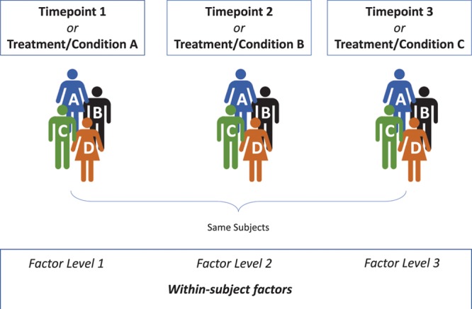
Schematic representation of a one-way repeated-measures ANOVA. An outcome is repeatedly measured or observed for each subject (here: subjects A–D) at each time point or under each condition, allowing to assess how the outcome value changes within each subject. Therefore, a factor in which each subject’s outcome variable is repeatedly measured at each factor level (here: time point or condition), is referred to as a within-subject factor. One-way repeated-measures ANOVA compares the mean values of the outcome variable between the factor levels. ANOVA indicates analysis of variance.

Figure 2.

Schematic representation of a two-way (two-factor) mixed ANOVA. The model includes a within-subject factor (Figure 1), but also a between-subject factor. Factors that vary between subjects are between-subject factors (here: a part of the subjects are assigned to treatment A, but other subjects are assigned to treatment B). A two-way mixed ANOVA tests for differences in the mean values of the outcome variable between the factor levels of the within-subject factor, between the factor levels of the between-subject factor, as well as the interaction of the 2. ANOVA indicates analysis of variance.

One-way repeated-measures ANOVA can be used either (1) to compare means in which some outcome has been measured in the same subjects under different conditions (eg, different treatments) or (2) to assess differences in an outcome serially measured at different time points in the same subjects (Figure 1).¹⁹ The tested null hypothesis is that all related means are equal.¹⁹

Unfortunately, while ANOVA gives an overall P value, it does not identify which group means are equal or not. A common approach to answer this question is to perform post hoc tests, which are pairwise comparisons of either selected means of interest or all possible combinations of means.²¹ Note that this involves testing of multiple null hypotheses, which leads to an inflated risk of a type I error—unless the significance criterion is adjusted accordingly. A more detailed discussion on multiple testing is found elsewhere.²²

Commonly, researchers aim to compare 2 or more groups (eg, treatment groups) in which the outcome is repeatedly assessed over time. There are thus 2 factors of interest in the repeated-measures design (time and treatment).¹⁹ Such a study design is traditionally analyzed with two-way (two-factor) repeated-measures ANOVA (Figure 2).^6,19 This ANOVA model simultaneously tests several null hypotheses: (1) all means at different time points are the same (referred to as “main effect of time”); (2) all means in different treatment groups are the same (referred to as “main effect of treatment”); and (3) there is no interaction between treatment and time (the treatment groups do not differ in their degree of change in the outcome variable over time).¹⁹ The interaction is often the primary interest when researchers aim to study whether treatments differentially affect outcomes over time.¹

Repeated-measures ANOVA techniques make quite strong assumptions about the underlying data. One important assumption is that the correlation between repeated measurements for the same subject is constant, irrespective how far apart in time the measurements are made (termed “compound symmetry correlation structure”).²³ The closely related assumption of sphericity means that the variances of the differences between any 2 time points is the same, irrespective of how distant the measurements are.²⁴ Violations of these assumptions are common because correlation between repeated data tend to be highest between adjacent time points and decrease with increasing time intervals, markedly increasing the risk of false-positive claims (type I error).¹ Mauchly’s test can be used to test for sphericity,²⁵ and adjustments, such as the Greenhouse and Geisser correction, can be applied when the assumption of sphericity is violated.²⁴

In studying the effects of therapeutic ultrasound and treadmill exercise in a rat model of neuropathic pain, Huang et al²⁶ repeatedly measured mechanical and thermal hypersensitivity as well as various cytokine levels. Outcomes were compared across 7 groups by repeated-measured ANOVA. The sphericity assumption was tested using Mauchly’s test, and Greenhouse–Geisser–corrected P values were presented when applicable. The authors observed significant differences between the groups for all outcomes and used post hoc analyses for pairwise comparisons between groups.²⁶

Multivariate ANOVA (MANOVA) does not assume a specific correlation structure or sphericity and is therefore a popular alternative to repeated-measures ANOVA.²³ Similarly to ANOVA, MANOVA also tests for main effects as well as for the interaction.^6,24 However, MANOVA also shares many of the limitations of ANOVA described in the next paragraph. Note that the term “multivariate” is commonly misused in literature to describe models with multiple independent (predictor) variables. In reality, multivariate means that there are multiple (correlated) outcomes—like an outcome repeatedly measured over time.

Despite its appeal and popularity, ANOVA has several shortcomings or limitations:

• The outcome must be continuous and should generally be normally distributed around the mean value at each factor level (unless the sample size is reasonably large).^1,7

• The within- and between-subject factors are categorical variables, and standard ANOVA models do not accommodate for continuous covariates.

• ANOVA cannot handle covariates that vary over time.⁷

• ANOVA assumes each individual to be measured at the same time points and does not allow for unequally spaced time intervals in different subjects.

• Measurements must be available for each subject at each time point, thus excluding the entire subject from the analysis when a single observation is missing.^1,23 Missing observations are quite common in repeated-measures designs (eg, due to logistic reasons, withdrawal, or loss to follow-up).²⁷

• ANOVA tests for “significance,” but does not allow inferences on how the outcome is expected to change as the predictor variable(s) change.

Nonparametric alternatives to the paired t test (Wilcoxon signed-rank test) and repeated-measures ANOVA (Friedman test) are available when the assumption of normally distributed residuals is violated.²⁸ However, these techniques do not address many of the other above limitations.

The following section deals with more modern and flexible but rather complex approaches that can (1) model a broad range of outcome data, including continuous, categorical, and count data; (2) accommodate categorical and continuous covariates; and (3) make use of all available information for each subject, even when measurements are unequally spaced or when a portion of the outcome data are missing. This remaining section is admittedly not basic material but is included for completeness sake.

MODERN APPROACHES OF COMPARING NONINDEPENDENT MEANS FOR LONGITUDINAL DATA

Regression Techniques for Correlated Data: Background

Linear regression allows one to model a continuous dependent (outcome) variable as a linear function of ≥1 independent variables.⁵ While ANOVA models can be expressed in terms of linear regression, regression is more flexible as it can include multiple categorical and/or continuous independent variables at the discretion of the investigator—for example, because they are of specific scientific interest or to adjust for confounding.⁵ Linear regression can also model nonlinear relationships—for example, by including the squared values of a predictor variable.⁵ Moreover, the concept can be generalized from continuous outcomes to other distributions including count data (Poisson regression) or binary outcomes (logistic regression).⁵ However, regression models generally assume measurements to be independent from each other.⁵ As detailed above, repeated measurements clearly violate this assumption.

There are 2 commonly used modern approaches that make use of the flexibility of regression models while accounting for nonindependent measurements.

The first approach focuses on specifying the mean response of the outcome (thus called a marginal approach or population-average approach), while using a technique to estimate the regression parameters that is valid in the presence of correlated measurements.^1,7 A generalized estimating equation (GEE) is commonly used to estimate the parameters in a marginal model, in combination with so-called robust standard errors to quantify the precision of the estimate.²

The second approach is not limited to the mean response but fully specifies the distribution of the outcome by using random intercepts and/or slopes.²⁹ Such subject-specific models have also variously been termed mixed-effect models, multilevel models, hierarchical models, or random-effects models.³⁰

Choosing which approach to apply partly depends on the aim of the research and the desired interpretation of the estimated effects (population-average versus subject-specific interpretation).

Marginal Models: GEEs

A GEE can be used to estimate the regression parameters for the expected (mean) response of an outcome given a set of explanatory variables while accounting for repeated measurements on same subjects.^2,31 To account for nonindependence, the analyst needs to specify a working correlation structure, which represents the assumed correlation of the repeated measurements.⁷ Figure 3 shows a schematic representation of a selection of different working correlation structures.

Figure 3.

Schematic representation of 4 working correlation structures commonly used in GEE estimation (A–D). The numbers 1–5 represent repetitive measurements, and the shade of the box represents the correlation between the 2 measurements, with a darker shade representing a stronger correlation. For example, the box on the cut-point between first row and third column (or vice versa) represents the correlation between the first and third measurements. While the correlation of a value with itself is always 1 (represented by the black boxes on the diagonal line), the off-diagonal correlations differ between the correlation structures. A, The independent correlation structure assumes uncorrelated measurements. B, Compound symmetry assumes all off-diagonal correlations to be equal. C, The autoregressive structure assumes decreasing correlations as the time interval increases. D, Unstructured correlation makes no assumptions and allows all correlations to differ. GEE indicates generalized estimating equation.

The exchangeable structure (also termed “compound symmetry”) assumes all correlations to be equal. The autoregressive structure assumes correlations to decrease as the time interval between the measurements increases. An unstructured correlation makes no assumptions about the structure and allows each correlation to be different.⁷ The GEE procedure, using robust standard errors, has the desirable property that its estimates are rather robust against misspecifications of the working correlation structure, and it will often still produce valid results, especially when the sample size is reasonably large.^2,7

As the marginal approach models the mean response, the interpretation refers to population-average effects of the predictor variables.⁷ The regression parameters thus allow inferences on how the mean outcome, averaged over the whole population, is expected to change relative to changes in the independent variable(s).⁷

Limitations of marginal models include that they only account for 1 source of nonindependence at a time (eg, repeated measurements in individuals). However, there may be other sources of nonindependence—for example, if the individuals in whom repeated measurements were made are also organized in other clusters, such as families, clinics, or hospitals. Mixed-effect models, described below, can accommodate several sources of nonindependence at once and allow for subject-specific conclusions.⁹

In studying whether a single-injection lumbar plexus block (LPB) would reduce postoperative pain after hip arthroscopy, YaDeau et al³² randomly assigned patients to receive either LPB or not. Postoperative pain scores (on a Numeric Rating Scale) were repeatedly assessed in the first 24 hours after surgery. Using the GEE approach with an autoregressive working correlation structure and adjusting for multiple covariates, LPB was associated with a mean pain reduction of 0.9 points (95% confidence interval, 0.1–1.7; P = .037).³²

Mixed-Effect Models

Mixed-effect models use a conceptually different approach than marginal models to account for nonindependence of repeated measurements. While marginal models focus on the mean outcome, mixed-effect models provide a fully specified model for the multivariate distribution of the repeatedly measured outcome.²⁹

There are 2 main types of comparative research studies involving longitudinal data, both of which often use mixed-effects models. First, researchers may simply want to compare treatments on the mean of the outcome while accounting for the repeated measurements over time (with time as a categorical variable), collapsing the data over time if there is no group-by-time interaction, but comparing groups over time if the effect differs over time. This could be accomplished with a GEE model, but also with a mixed-effects model, which can incorporate random effects to account for within-subject or within-unit clustering, while still allowing all of the within-subject correlation modeling as in a GEE model.

Second, researchers may be interested in comparing groups on the trends over time in the outcome, and thus include time as a continuous variable. In a mixed-effect model, each subject’s deviation from the mean slope and the beginning point (the intercept) can be modeled using a random intercept and random slope model, as detailed below.

Thus, in a mixed-effects model, one can (1) model the within-subject correlation in which one specifies the correlation structure for the repeated measurements within a subject (eg, autoregressive or unstructured) and/or (2) control for differences between individuals by allowing each individual to have its own regression line (Figure 4).⁶ By accounting for the fact that some individuals have consistently higher (or lower) values than others—by allowing for an individual intercept—a mixed-effect model controls for this source of variation. Likewise, individual slopes can be included in the model to control for the fact that individual responses over time differ among subjects (Figure 4).

Figure 4.

Simple example with only 1 explanatory variable (time as continuous covariate) to illustrate how linear regression assuming independent measurements differs from a mixed linear model. A, All data points are assumed to be independent. The solid line represents the regression line of the relationship between time and a hypothetical outcome measure. The difference (vertical distance) between each point and the regression line is termed residual, and the assumption of independence that we have rather informally stated in the text actually refers to independence of the residuals. As can be seen, the line does not seem to fit the data points very well, and the variance of the residuals seems to increase over time, violating a key assumption of linear regression. B, It can be see that the different data points in (A) are not independent but actually come from 4 subjects (represented by 4 different symbols and colors), measured at hourly intervals. The black line still represents the mean change in the dataset. However, by allowing each subject to have its own intercept and slope, the between-subject variability is now accounted for. The residuals are now much smaller as they represent the within-subject variability, ie, the difference of each data point from the regression line of the same subject. This allows for a more precise estimate of the subject-specific effect of time.

Since the individuals are usually a random sample from all possible individuals of a population, their individual slopes and intercepts are usually of no specific interest. The aim is simply to control for the variation coming from different subjects, which can be achieved by modeling subject effects as if they randomly came from a probability distribution (random effects).³³ In contrast to these random effects, effects of covariates that are of specific scientific interest and that comprise all levels, or the whole range of values, about which inferences are to be made (eg, treatment groups, age, sex) are referred to as fixed effects.³³ The name mixed-effect models arises from the fact that they include both fixed and random effects.⁶ Of note, when fitting a random slope model, one also includes the fixed effect for time. The fixed effect of time (as continuous variable) then estimates the average change over time, or average slope, across the subjects.

Building a mixed-effect model requires informed choices not only on which fixed effects to include but also on whether to include random intercepts or slopes, or both. Mixed-effect models can also accommodate multiple levels of nonindependence by including additional random effects (eg, not only for participants, but also for ≥1 other clusters) to the model.⁹ As an additional complexity, random intercepts and random slopes are often correlated with each other, and this correlation also needs to be accounted for.²⁹

The various possibilities and choices in building a mixed-effect model are major strengths because they provide great flexibility and allow modeling subject-specific trajectories over time, as well as modeling the correlation between measurements within subject. Nevertheless, this can also be a limitation as misspecifications of the model can lead to biased estimates and wrong inferences.

Effects estimated by mixed-effect models basically have a subject-specific interpretation, in the sense that they represent the expected change in the dependent variable for a particular individual or cluster of individuals.³⁴ However, it is also possible to derive population-average estimates in mixed-effect models. While subject-specific and population-averaged estimates are identical in linear mixed models for normally distributed outcome data, the distinction is relevant for noncontinuous outcomes (eg, mixed logistic model for binary outcomes).³⁵ The relative merits of the mixed-effect model approach and the marginal approach compared to each other, as well as differences in interpretation of the results, have been extensively debated elsewhere.^34–38

Upton et al³⁹ studied the “Analgesia Nociception Index” (ANI), a noninvasive measure of the nociceptive level of a given patient, to guide administration of analgesics in patients undergoing general anesthesia. The authors hypothesized that intraoperative ANI-guided fentanyl administration would reduce pain in the recovery room when compared to standard practice. They repeatedly recorded Numerical Rating Scale pain scores at 5-minute intervals in the recovery room from 0 to 90 minutes. A linear mixed-effect model was used for the analysis of the primary outcome, with ANI guidance being the fixed effect, and patients modeled as the random effect. ANI-guided fentanyl administration was associated with a significant reduction of postoperative pain scores (mean reduction in 1.3 units; P = .01).³⁹

POWER AND SAMPLE SIZE CONSIDERATIONS

As for an any study, a priori estimation of the required sample size requires researchers to make choices concerning the planned data analysis strategy and primary hypothesis that is to be tested, the acceptable type I error rate, the desired power, and the minimum important difference to be detected.⁴⁰ However, sample size calculations for repeated measurement designs also require specifications of the assumed variance and correlation pattern between repeated measurements.⁴¹ Full details are beyond the scope of this primer, and we refer to previous publications on sample size and power considerations for longitudinal designs.^40–42

CONCLUSIONS

Longitudinal study designs are common when investigating changes in an outcome over time. Their proper data analysis needs to account for the correlation among repeatedly measured data. A simple and intuitive approach involves calculation of a summary statistic to summarize the repeatedly measured data in each subject with a single number. This removes the correlation among the measurements and allows for a straightforward comparison of groups using standard, conventional statistical hypothesis tests. Repeated-measures ANOVA approaches have traditionally been used to analyze longitudinal data. However, strong data assumptions and minimal flexibility limit the usefulness. Modern approaches are becoming more accessible to statisticians and thus researchers and are increasingly superseding the more traditional methods. GEEs allow valid estimations of regression parameters for the mean response of the outcome in the presence of nonindependent measurements. Mixed-effect models provide a fully specified model of the distribution of the outcome, can be used to estimate the between-subject variation, and are more appropriate when the research focuses on within-subject change. With the above specific examples of studies published in Anesthesia & Analgesia, we show how these techniques are successfully applied in practice.

DISCLOSURES

Name: Patrick Schober, MD, PhD, MMedStat.

Contribution: This author helped write and revise the manuscript.

Name: Thomas R. Vetter, MD, MPH.

Contribution: This author helped write and revise the manuscript.

This manuscript was handled by: Jean-Francois Pittet, MD.

REFERENCES

- 1.Ma Y, Mazumdar M, Memtsoudis SG. Beyond repeated-measures analysis of variance: advanced statistical methods for the analysis of longitudinal data in anesthesia research. Reg Anesth Pain Med. 2012;37:99–105.. [DOI] [PMC free article] [PubMed] [Google Scholar]
- 2.Albert PS. Longitudinal data analysis (repeated measures) in clinical trials. Stat Med. 1999;18:1707–1732.. [DOI] [PubMed] [Google Scholar]
- 3.Mascha EJ, Sessler DI. Equivalence and noninferiority testing in regression models and repeated-measures designs. Anesth Analg. 2011;112:678–687.. [DOI] [PubMed] [Google Scholar]
- 4.Zeger SL, Liang KY. An overview of methods for the analysis of longitudinal data. Stat Med. 1992;11:1825–1839.. [DOI] [PubMed] [Google Scholar]
- 5.Vetter TR, Schober P. Regression: the apple does not fall far from the tree. Anesth Analg. 2018;127:277–283.. [DOI] [PubMed] [Google Scholar]
- 6.Fitzmaurice GM, Ravichandran C. A primer in longitudinal data analysis. Circulation. 2008;118:2005–2010.. [DOI] [PubMed] [Google Scholar]
- 7.Ballinger GA. Using generalized estimating equations for longitudinal data analysis. Organ Res Methods. 2004;7:127–150.. [Google Scholar]
- 8.Liang KY, Zeger SL. Regression analysis for correlated data. Annu Rev Public Health. 1993;14:43–68.. [DOI] [PubMed] [Google Scholar]
- 9.De Livera AM, Zaloumis S, Simpson JA. Models for the analysis of repeated continuous outcome measures in clinical trials. Respirology. 2014;19:155–161.. [DOI] [PubMed] [Google Scholar]
- 10.Dickinson LM, Basu A. Multilevel modeling and practice-based research. Ann Fam Med. 2005;3suppl 1S52–S60.. [DOI] [PMC free article] [PubMed] [Google Scholar]
- 11.Vetter TR. Fundamentals of research data and variables: the devil is in the details. Anesth Analg. 2017;125:1375–1380.. [DOI] [PubMed] [Google Scholar]
- 12.Mascha EJ, Vetter TR. Significance, errors, power, and sample size: the blocking and tackling of statistics. Anesth Analg. 2018;126:691–698.. [DOI] [PubMed] [Google Scholar]
- 13.Schober P, Bossers SM, Schwarte LA. Statistical significance versus clinical importance of observed effect sizes: what do P values and confidence intervals really represent? Anesth Analg. 2018;126:1068–1072.. [DOI] [PMC free article] [PubMed] [Google Scholar]
- 14.Schober P, Boer C, Schwarte LA. Correlation coefficients: appropriate use and interpretation. Anesth Analg. 2018;126:1763–1768.. [DOI] [PubMed] [Google Scholar]
- 15.Rogge DE, Nicklas JY, Haas SA, Reuter DA, Saugel B. Continuous noninvasive arterial pressure monitoring using the vascular unloading technique (CNAP System) in obese patients during laparoscopic bariatric operations. Anesth Analg. 2018;126:454–463.. [DOI] [PubMed] [Google Scholar]
- 16.Vetter TR, Schober P. Agreement analysis: what he said, she said versus you said. Anesth Analg. 2018;126:2123–2128.. [DOI] [PubMed] [Google Scholar]
- 17.Senn S, Stevens L, Chaturvedi N. Repeated measures in clinical trials: simple strategies for analysis using summary measures. Stat Med. 2000;19:861–877.. [DOI] [PubMed] [Google Scholar]
- 18.Matthews JN, Altman DG, Campbell MJ, Royston P. Analysis of serial measurements in medical research. BMJ. 1990;300:230–235.. [DOI] [PMC free article] [PubMed] [Google Scholar]
- 19.Sullivan LM. Repeated measures. Circulation. 2008;117:1238–1243.. [DOI] [PubMed] [Google Scholar]
- 20.Vetter TR, Mascha EJ. Unadjusted bivariate two-group comparisons: when simpler is better. Anesth Analg. 2018;126:338–342.. [DOI] [PubMed] [Google Scholar]
- 21.Liu C, Cripe TP, Kim MO. Statistical issues in longitudinal data analysis for treatment efficacy studies in the biomedical sciences. Mol Ther. 2010;18:1724–1730.. [DOI] [PMC free article] [PubMed] [Google Scholar]
- 22.Cabral HJ. Multiple comparisons procedures. Circulation. 2008;117:698–701.. [DOI] [PubMed] [Google Scholar]
- 23.Everitt BS. Analysis of longitudinal data. Beyond MANOVA. Br J Psychiatry. 1998;172:7–10.. [DOI] [PubMed] [Google Scholar]
- 24.Keselman HJ, Algina J, Kowalchuk RK. The analysis of repeated measures designs: a review. Br J Math Stat Psychol. 2001;54:1–20.. [DOI] [PubMed] [Google Scholar]
- 25.Mauchly JW. Significance test for sphericity of a normal n-variate distribution. Ann Math Stat. 1940;11:204–209.. [Google Scholar]
- 26.Huang PC, Tsai KL, Chen YW, Lin HT, Hung CH. Exercise combined with ultrasound attenuates neuropathic pain in rats associated with downregulation of IL-6 and TNF-α, but with upregulation of IL-10. Anesth Analg. 2017;124:2038–2044.. [DOI] [PubMed] [Google Scholar]
- 27.Ogenstad S. Analysis and design of repeated measures in clinical trials using summary statistics. J Biopharm Stat. 1997;7:593–604.. [DOI] [PubMed] [Google Scholar]
- 28.Gliner JA, Morgan GA, Harmon RJ. Single-factor repeated-measures designs: analysis and interpretation. J Am Acad Child Adolesc Psychiatry. 2002;41:1014–1016.. [DOI] [PubMed] [Google Scholar]
- 29.Bandyopadhyay S, Ganguli B, Chatterjee A. A review of multivariate longitudinal data analysis. Stat Methods Med Res. 2011;20:299–330.. [DOI] [PubMed] [Google Scholar]
- 30.Lininger M, Spybrook J, Cheatham CC. Hierarchical linear model: thinking outside the traditional repeated-measures analysis-of-variance box. J Athl Train. 2015;50:438–441.. [DOI] [PMC free article] [PubMed] [Google Scholar]
- 31.Zeger SL, Liang KY. Longitudinal data analysis for discrete and continuous outcomes. Biometrics. 1986;42:121–130.. [PubMed] [Google Scholar]
- 32.YaDeau JT, Tedore T, Goytizolo EA, et al. Lumbar plexus blockade reduces pain after hip arthroscopy: a prospective randomized controlled trial. Anesth Analg. 2012;115:968–972.. [DOI] [PubMed] [Google Scholar]
- 33.Littell RC, Milliken GA, Stroup WW, Wolfinger RD, Schabenberger O. Introduction. SAS for Mixed Models. 2006:Cary, NC: SAS Institute; 1–16.. [Google Scholar]
- 34.Hu FB, Goldberg J, Hedeker D, Flay BR, Pentz MA. Comparison of population-averaged and subject-specific approaches for analyzing repeated binary outcomes. Am J Epidemiol. 1998;147:694–703.. [DOI] [PubMed] [Google Scholar]
- 35.Neuhaus JM, Kalbfleisch JD, Hauck WW. A comparison of cluster-specific and population-averaged approaches for analyzing correlated binary data. Int Stat Rev. 1991;59:25–35.. [Google Scholar]
- 36.Hubbard AE, Ahern J, Fleischer NL, et al. To GEE or not to GEE: comparing population average and mixed models for estimating the associations between neighborhood risk factors and health. Epidemiology. 2010;21:467–474.. [DOI] [PubMed] [Google Scholar]
- 37.Zeger SL, Liang KY, Albert PS. Models for longitudinal data: a generalized estimating equation approach. Biometrics. 1988;44:1049–1060.. [PubMed] [Google Scholar]
- 38.Lee Y, Nelder JA. Conditional and marginal models: another view. Stat Sci. 2004;19:219–238.. [Google Scholar]
- 39.Upton HD, Ludbrook GL, Wing A, Sleigh JW. Intraoperative “Analgesia Nociception Index”-guided fentanyl administration during sevoflurane anesthesia in lumbar discectomy and laminectomy: a randomized clinical trial. Anesth Analg. 2017;125:81–90.. [DOI] [PubMed] [Google Scholar]
- 40.Guo Y, Logan HL, Glueck DH, Muller KE. Selecting a sample size for studies with repeated measures. BMC Med Res Methodol. 2013;13:100. [DOI] [PMC free article] [PubMed] [Google Scholar]
- 41.Guo Y, Pandis N. Sample-size calculation for repeated-measures and longitudinal studies. Am J Orthod Dentofacial Orthop. 2015;147:146–149.. [DOI] [PubMed] [Google Scholar]
- 42.Liu G, Liang KY. Sample size calculations for studies with correlated observations. Biometrics. 1997;53:937–947.. [PubMed] [Google Scholar]