Assessing the performance of docking scoring function, FEP, MM-GBSA, and QM/MM-GBSA approaches on a series of PLK1 inhibitors

The ranking capability of FEP is the best with r_s = 0.854. QM/MM-GBSA can reach 0.767 with much lower computation time.

Abstract

Over-expressed polo-like kinases 1, a key regulator of cell mitosis, is associated with carcinogenesis and poor prognosis. It is very necessary to develop a reliable computational affinity prediction protocol targeting PLK1. In this study, the performance of different docking scoring function, free energy perturbation, MM-GBSA and QM/MM-GBSA were evaluated. The ranking capability of FEP is the best with r_s = 0.854. However, the r_s obtained from MM-GBSA can reach 0.767, which requires only about one-eighth of the simulation time of FEP. As for the sampling method, single long molecular dynamics (SLMD) surpass the multiple short molecular dynamics (MSMD) in ranking of the 20 congeneric compounds by about 0.1 in r_s. In addition, ligands treated by QM can significantly improve the ranking performance. As for the docking scoring functions, a force field-based scoring function is more suitable for ranking congeneric compounds.

Introduction

Polo-like kinases 1 (PLK1) is a well-characterized member of the serine/threonine kinases PLK family, which is highly conserved among eukaryotes. PLK1 has been identified as a key regulator of cell mitosis. It mediates a variety of cell cycle events, including mitotic entry, centrosome duplication, bipolar mitotic spindle formation, transition from metaphase to anaphase, cytokinesis, and maintenance of genomic stability.1–4 Furthermore, recent studies suggest that PLK1, beyond its traditional function in mitosis, is also involved in the DNA damage response, carcinogenesis, and early embryonic development.5 In about 80% of human tumors of various origins (lung, breast, ovary, colon, stomach, and esophagus), PLK1 is over-expressed.6 In addition, over-expression of PLK1 is associated with a poor prognosis in several tumor types and a lower overall survival rate.7,8 The over-expression studies of PLK1 in cancer cell lines (MCF-7 breast, Hela S3 cervical, SW-480 colon, and A549 lung cancer) show that the loss of PLK1 over-expression can induce pro-apoptotic pathways and inhibit growth by mitotic chaos and severe perturbance of cell cycle progression.9 The crystal structure of the kinase domain for PLK1 has been reported in detail.10 Hence, PLK1 is one of the most attractive and promising targets for antitumor drug development. More novel and selective small molecule inhibitors of PLK1 will offer new hope for cancer patients in the future.

To decrease the cost of synthesis and biological activity testing, it is necessary to develop a reliable computational affinity prediction protocol targeting PLK1. The embedded scoring functions of docking packages are rapid and suitable for virtual screening, but have poor precision.11 Free energy perturbation (FEP), having the most stringent theoretical background, is suitable for the evaluation of relative binding energies of congeneric compounds, but it demands large computational resources.12 MMG(P)BSA achieves a balance between speed and accuracy, which can be used for further selection of candidates from the result of virtual screening.13 The performance of MM/PBSA and MM/GBSA methods was evaluated by Hou's group systematically.14–18 These studies provide useful guidance for the use of MMG(P)BSA. However, simulation length, implicit solvent model, radii, and sampling protocols affect the prediction quality of MM-GBSA dramatically.19 In addition, recent studies suggested that multiple independent molecular dynamics can explore conformational space more effectively than single long molecular dynamics, and thus can provide better convergence and accuracy.20 Because of the semi-empirical calculation of a crucial amide acid and binding ligand in place of the empirical small molecular force field, the QM/MM-GBSA method is assumed to outperform the MM-GBSA method.21

Within this context, to investigate the difference in the accuracy of docking scoring functions, MMG(P)BSA and FEP against congeneric compounds, and moreover, to explore what is the best combination of radii settings, QM Hamiltonians, implicit solvent methods and simulation length of the system and whether multiple independent sampling improves the prediction of binding free energy compared to the use of one long simulation for the studied system, we conducted a series of comparative trials using the PLK1 structure and 20 congeneric compounds with known affinity.

Results and discussion

Molecular docking

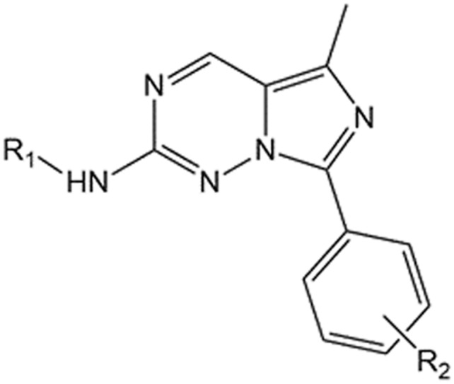
All molecules adopt similar docking modes, with the imidazo[1,5-f][1,2,4]triazine scaffold forming two hydrogen bonds with Cys133 (Fig. 1) and interacting with Phe183 with π–π stacking. Moreover, as for compounds with higher potency, taking compound 15E as an example, the methoxyl groups of the benzyl group on 2-NH form the other two hydrogen bonds with Arg57, making them more stable. In addition to that, the 7-substituted benzyl group is expected to form the hydrophobic interaction with Cys67 and Leu59. As for compound 20, because of the loss of a benzyl group on 2-NH, the hydrogen bond with Arg57 and hydrophobic interaction with Leu59 is not established, thus leading to very poor activity.

Fig. 1. Docking conformations of imidazo[1,5-f][1,2,4]triazine derivatives.

FEP binding affinity calculation

In FEP calculation, the above docking conformations were used as the initial binding poses. A single 5 ns simulation for each of the 12 λ windows was used, leading to a total of 60 ns of cumulative simulation time per perturbation. FEP implementation was based on OPLSv3, Desmond GPU MD engine and REST sampling. All FEP perturbations were performed in both solvent and protein. With compound 1 as the reference structure, 19 compounds were calculated. The predicted ΔG (kcal mol^–1) and the experimental ΔG are shown in Table 1 and Fig. 2. The r_s-FEP is 0.854, and the correlation R² is 0.852, with MUE compared to the experimental value of 0.58 kcal mol^–1. The solvent and complex contributions with the standard deviations are presented in Fig. S1.†

Table 1. The structures of 20 imidazo[1,5-f][1,2,4]triazine derivatives and the r_s obtained from FEP, docking scoring function and MM-GBSA.

Cpd.	R1	R2	Experimental	FEP	ChemPLP	Autodock4	Amberscore	Vina local	MSMDmbondi_PM3_igb5	SLMDmbondi2_PM6_igb5
1	–Ph	H	–8.1276	–8.12756 ± 0.10	73.6364	–6.58	–33.7883	–9.3791	–40.7684 ± 1.6668	–33.4167 ± 3.0057
2	–(3-OMe)Ph	H	–8.9540	–8.96756 ± 0.07	73.8094	–7.38	–33.2232	–9.1718	–42.4805 ± 1.9925	–34.0891 ± 3.1157
3	–(4-OMe)Ph	H	–8.4662	–9.22756 ± 0.08	78.4479	–6.81	–36.7728	–9.4601	–43.1313 ± 1.6334	–33.5346 ± 3.8370
4	–(4-O-CH2CH2N(Me)2)Ph	H	–8.8131	–9.78756 ± 0.08	86.2887	–6.7	–51.8358	–8.7975	–51.0326 ± 2.9872	–35.3578 ± 4.1413
5	–(3-CF3)Ph	H	–6.8635	–8.04756 ± 0.07	68.3719	–6.18	–29.7214	–9.4204	–40.8781 ± 1.9227	–32.9662 ± 3.0469
6	–(4-NO2)Ph	H	–7.6203	–8.74756 ± 0.07	79.4	–6.55	–35.2479	–9.5531	–38.8696 ± 1.3642	–32.999 ± 3.4822
7	–(4-SO2NH2)Ph	H	–7.6354	–7.22756 ± 0.12	81.5409	–6.4	–32.4445	–9.8944	–39.066 ± 3.4654	–27.4656 ± 6.6675
8	–(3,4-DiOMe)Ph	H	–9.6718	–10.21756 ± 0.08	83.034	–7.38	–38.4054	–9.7656	–47.4319 ± 1.8558	–34.6073 ± 3.4447
9	–(3,4,5-TriOMe)Ph	H	–10.1552	–9.87756 ± 0.09	82.0398	–7.76	–37.5877	–9.5219	–49.0133 ± 2.1209	–33.8125 ± 3.9465
10	–(3,4,5-TriOMe)Ph	2-OMe	–7.2029	–7.71756 ± 0.09	86.8232	–7.87	–39.1424	–9.461	–47.2244 ± 2.7552	–29.2794 ± 3.7124
11	–(3,4,5-TriOMe)Ph	2-NO2	–7.8290	–7.38756 ± 0.07	86.4641	–8.31	–42.2286	–9.8871	–46.3883 ± 2.5109	–35.7643 ± 7.4702
12	–(3,4,5-TriOMe)Ph	2-Br	–7.6508	–6.98756 ± 0.06	83.5109	–8.1	–42.3043	–9.8587	–49.1359 ± 2.6631	–33.4484 ± 3.9613
13	–(3,4,5-TriOMe)Ph	3-Br	–9.8216	–11.22756 ± 0.07	79.357	–7.65	–39.5474	–9.562	–53.52 ± 2.2223	–41.4111 ± 3.9253
14	–(3,4,5-TriOMe)Ph	3-CF3	–10.3267	–10.48756 ± 0.06	82.5021	–7.5	–38.2151	–9.6901	–54.4863 ± 2.7162	–38.8999 ± 3.7321
15	–(3,4,5-TriOMe)Ph	4-CF3	–8.2015	–8.69756 ± 0.06	59.8354	–7.51	–32.8453	–8.5513	–50.6827 ± 2.456.	–37.4751 ± 3.9192
16	–(3,4,5-TriOMe)Ph	3-C(O)Ph	–8.7678	–9.02756 ± 0.12	85.7232	–8.71	–36.9219	–10.2017	–50.8098 ± 3.1479	–37.5983 ± 4.5517
17	–(3,4,5-TriOMe)Ph	3-O-Ph	–8.6495	–10.26756 ± 0.08	81.7089	–8.25	–39.1877	–9.788	–52.8585 ± 2.3628	–38.5518 ± 3.6208
18	–(3,4,5-TriOMe)Ph	4-F	–9.7420	–9.68756 ± 0.05	79.8376	–7.67	–34.7426	–9.6023	–48.1593 ± 2.7720	–36.1043 ± 3.7958
19	–CH2Ph	H	–7.9945	–7.32756 ± 0.10	73.5278	–7.03	–35.0849	–8.9905	–41.0929 ± 1.5648	–31.9667 ± 3.2852
20	H	H	–3.1586	–3.13756 ± 0.10	46.6492	–4	–25.4246	–7.0976	–28.9258 ± 1.2683	–22.7462 ± 3.0669
r s a				0.854	0.217	0.378	0.34	0.171	0.698	0.767

^a r _s represents Spearman ranking coefficient. The standard deviations of MS(SL)MD were calculated based on 50 repeats.

Fig. 2. Correlation between predicted FEP and experimental binding energy for the 20 imidazo[1,5-f][1,2,4]triazine derivatives.

Comparison of the performance of four docking scoring functions

ChemPLP is an empirical scoring function, which uses the piecewise linear potential (PLP) scoring function to model steric complementarity of the protein and the ligand. Moreover, it adopts terms of GOLD's Chemscore implementation to introduce angle-dependent terms for hydrogen bonding and metal binding. It also employs the torsional potential from the Tripos force field together with a heavy-atom clash term to account for intraligand interactions. The r_s-ChemPLP is 0.217, which is much lower than r_s-FEP. The scoring function embedded in Autodock vina is another empirical scoring function, which is similar to X-score, but it counts the intermolecular and intramolecular contributions simultaneously that can avoid severe internal clash. The r_s-vina is 0.171.

AutoDock 4.2 uses a semi-empirical free energy force field to evaluate conformations during docking simulations, whose terms include evaluations for dispersion/repulsion, hydrogen bonding, electrostatics, and desolvation. The r_s-Autodock is 0.378. The AMBER score is a force field-based scoring function, which calculates the interaction between the ligand and the receptor by electrostatic, van der Waals energy terms, and the solvation energy using a generalized Born (GB) solvation model. The calculation uses the following protocol: minimization with a conjugate gradient method, followed by MD simulation (Langevin molecular dynamics at constant temperature), another minimization, and a final energy evaluation. The main advantage of the Amber score is that during the MD simulation, both the ligand and the active site of the receptor can be flexible, allowing small structural rearrangements to reproduce the so-called “induced fit” while performing the scoring. The r_s-Amber score is 0.347. Reviewing the abovementioned four docking scoring functions, it has been found that the force field-based scoring methods such as Amber score and the Autodock 4 scoring function outperformed the empirical methods like ChemPLP and vina score in ranking the potency of the congeneric compounds.

The effect of MD simulation length on MM-G(P)BSA

The r_s between the experimental and predicted binding free energies using different MD trajectory lengths in MM-G(P)BSA calculations are depicted in Fig. 3. It can be seen that for the PBSA method, even 10 ns is not enough to get the optimal r_s, while for GBSA, 8 ns seemed to be a plausible choice in getting the ideal result.

Fig. 3. The variation of r_s with the length of the production simulation.

Comparison of radii sets, generalized Born methods, QM/MM-GBSA and multiple short MD simulation

Generally, SLMD surpasses the MSMD in ranking of the 20 congeneric compounds by about 0.1 in r_s. SLMD and MSMD have a similar response for different radii sets, different generalized Born methods and different QM method (Fig. 4). Specifically, as for the radii sets, mbondi is better than bondi, while bondi is similar to mbondi2. Overall, the QM/MM-GBSA method is significantly better than MM-GBSA by about 0.2 in r_s. As far as the semi-empirical QM theory levels were concerned, the PM3 method seemed to outperform the AM1 and PM6 methods. As for the generalized Born model, it depends on the sampling and molecular mechanics (MM) methods. In the MM and AM1 methods, generally, for the SLMD and MSMD, igb1 < igb2 < igb5, except for MSMD-mbondi2 with MM method. It should be noted that for SLMD, the mbondi method is more sensitive to the generalized Born method. In MM, when igb = 1, the r_s is 0.528; when igb = 2, the r_s is 0.659; when igb = 5, the r_s is up to 0.722, which is higher than that of igb1 by 0.2. As for AM1, a similar phenomenon was observed. When igb = 1, the r_s is 0.635, but when igb = 5, the r_s reaches 0.752. In the PM3 method, for MSMD, igb1 < igb2 < igb5, while for SLMD, igb1 < igb5 < igb2. It should be noted that there are two coincidence points in igb1 and igb5, that is to say, the radii sets have no influence on the ranking when using PM3 and SLMD sampling. In PM6, the result is complex. As for MSMD, igb5 > igb1 ≈ igb2, while for SLMD, for mbondi, igb1 < igb5 < igb2; for bondi, igb2 < igb1 < igb5; for mbondi2, igb1 < igb2 < igb5. The optimal r_s of SLMD is 0.767 when using the mbondi2, PM6 and igb5 method, which is higher than that of MSMD by 0.069 using mbondi, PM3 and the igb5 method (Table 2). It was found that although the r_s of SLMD is better than MSMD, the standard deviation of the binding energy predicted by the SLMD is significantly larger than that of MSMD.

Fig. 4. The variation of r_s with the different radii, GB model, QM, and sampling method.

Table 2. The spearman coefficient of experimental and predicted binding free energies of different radii sets, GB model, QM and sampling method.

	igb = 1	igb = 2	igb = 5	AM1 igb = 1	AM1 igb = 2	AM1 igb = 5
RM-mbondi	0.474	0.528	0.544	0.558	0.627	0.642
RM-bondi	0.451	0.477	0.489	0.558	0.588	0.602
RM-mbondi2	0.444	0.495	0.463	0.559	0.594	0.621
LM-mbondi	0.528	0.659	0.722	0.635	0.666	0.752
LM-bondi	0.562	0.592	0.627	0.603	0.641	0.662
LM-mbondi2	0.562	0.583	0.621	0.615	0.647	0.662

	PM3 igb = 1	PM3 igb = 2	PM3 igb = 5	PM6 igb = 1	PM6 igb = 2	PM6 igb = 5
RM-mbondi	0.614	0.662	0.698	0.583	0.567	0.641
RM-bondi	0.606	0.647	0.662	0.549	0.502	0.549
RM-mbondi2	0.606	0.662	0.66	0.576	0.555	0.576
LM-mbondi	0.666	0.747	0.719	0.668	0.761	0.743
LM-bondi	0.666	0.725	0.719	0.653	0.618	0.696
LM-mbondi2	0.666	0.737	0.719	0.654	0.701	0.767

Conclusions

The ranking capability of FEP is the best with r_s = 0.854. However, the r_s obtained from the 8 ns MD sampling-based MM-GBSA score can reach 0.767, which is lower than that of FEP by 0.087, but the computation time is much lower than that of FEP. In addition, as for MM-GBSA, ligands treated by QM can significantly improve the ranking performance. As far as QM is concerned, PM3 is more stable than AM1 and PM6. Mbondi is more sensitive to the generalized Born method, and the recommended igb is 5. Igb2 is appropriate for bondi and mbondi2. As for the docking scoring function, a force field-based scoring function is more suitable for ranking of the congeneric compounds. The reported results using FEP calculations are better than other approximate methods like DockScore, Amber score and QM/MM-GBSA, but the accuracy of the FEP results is not as high as one would have expected. This could be because of the issues with the force field parameters, and we believe that on using the QM/MM-based FEP method reported by Reddy's group,22,23 the accuracy of the FEP results could be improved.

Experimental

Computational docking procedure and scoring

Docking was performed using the GOLD software.24 The receptor X-ray structure was retrieved from ; RCSB.org with PDB code ; 2rku. The ions, water molecules and ligands were removed prior to docking. Default options were used unless otherwise noted. Moreover, 10 genetic algorithm dockings were conducted in a single run. The binding site point was set as –44.7010, 2.9850, 6.0460. All atoms within 6 Å of the ligands were used to define the binding site. The slow option was used for docking. The scoring function used was ChemPLP.25

With the above docking conformations, the binding affinities were also evaluated by Autodock4.2,26 Autodock Vina27 and Amber score embedded in DOCK6.28 Default parameters were used. As for Autodock Vina, the local_only parameter was used.

Complex preparation

The binding conformations of 20 compounds were taken from the abovementioned docking results. AM1-BCC charges were assigned to the ligands. The AMBER 99SB force field and the general AMBER force field (GAFF) parameters were assigned to the protein and the ligand using the antechamber in AMBER v11,29 respectively. A 10 Å TIP3P water molecule octahedron box was set to solvate the complex system along with Na⁺ and Cl^– counter-ions to neutralize the system.

Experimental enzymatic activity

The experimental inhibition data of the 20 compounds were taken from Cheung's study.30 The experimental free energies of binding were calculated from K_i using eqn (1), where R is the ideal gas constant (1.9872 × 10^–3 kcal K^–1 mol^–1) and T is 300 K. As for compound 5 and 20, only > 10 μM inhibition data was available. According to their binding modes and docking scores acquired from Autodock 4, we assumed that the IC₅₀ of compound 5 is 10 μM because its predicted affinity is close to compound 7 whose IC₅₀ is 2.74 μM. As for compound 20, because of the loss of a methoxyl benzyl moiety to interact with the crucial residue Asp57, the predicted binding energy of Autodock 4 is evidently higher than that of compound 5 by 1.82 kcal mol^–1; thus we assumed that the IC₅₀ of compound 20 is 5000 μM.

ΔG_bind = RT ln K_i 1

Computational FEP procedure

All calculations were conducted using Desmond version 3.9.31 OPLSv3 force field32 was used and the MD simulation was calculated by the GPU-enabled parallel molecular dynamics engine. Overall, the system is solvated by adding SPC water with a buffer distance of 5 Å for complexes and 10 Å for the pure solvent. The system was relaxed by two minimizations, followed by 4 short molecular dynamics simulations. The production simulation is run for 5 ns for each lambda window, and 12 windows are used for each perturbation, with the molecules in the chosen docked posing as the starting conformation. Proteins were prepared using the Protein Preparation Wizard in Maestro. In FEP calculations, compound 1 was set as the reference, and the ΔΔG_bind of the other 19 compounds was calculated. To avoid the larger mutation and enhance the prediction accuracy of the FEP, the mutation pathway and their ΔΔG_bind are described in Fig. S1.† Briefly, compound 20 was first mutated into compound 1 and compound 19. Then, on the basis of compound 1, R₂ was kept as H, and only minor changes were made in the benzene ring of R₁ to obtain compounds 2, 3, 5, 6, 7. Then, compound 3 was mutated into compound 4 and compound 8, and then compound 8 was further modified to form compound 9. Finally, according to compound 9, R₁ was kept as the –(3,4,5-TriOMe)Ph group, and R₂ was mutated to obtain compounds 10–18.

Molecular dynamics (MD) simulations

The systems were first minimized using 5000 steps (1000 steps of steepest descent minimization and 4000 steps of conjugate gradient method) with restraint_wt 500 kcal mol^–1 Å^–1 fixing the solution molecule to optimize the water molecules, followed by another 5000 steps with restraint force 10 kcal mol^–1 Å^–1 fixing the Cα and ligand to optimize the internal H bonds. After minimization, the system was heated from 0 to 300 K over 50 picoseconds (ps) using the NVT ensemble with a 10 kcal mol^–1 Å^–1 weak restraint on the kinase and ligands. Then, the systems were density equilibrated over 50 ps at constant pressure (1 bar) and temperature (300 K) with a 2 kcal mol^–1 Å^–1 on the complex. Next, 400 ps of NPT equilibration was conducted. Finally, a 10 nanosecond (ns) NPT production run was conducted. The long-range electrostatics were included by means of a particle mesh Ewald (PME) method, and the cutoff of 10 Å was used for all the MD simulations. All hydrogen-heavy atom bonds were constrained by the SHAKE method, and simulations were performed with a 2 fs time, and Langevin dynamics were used for temperature control.

MM-PBSA calculation

The MM-PBSA calculations were performed using MMPBSA.py in AMBERTools 12. The MM-PBSA surface tension (α) and the non-polar free energy correction term (β) were set to 0.00543 kcal mol^–1 Å^–1 and 0.92, respectively. An exterior dielectric constant of 80 and solute dielectric constant of 1 were used. 500 snapshots were taken evenly from the MD simulations trajectory from 0 to 10 ns in the MM-PBSA calculations.

MM-GBSA and QM/MM-GBSA calculation

The (QM)/MM-GBSA calculations were performed using MMPBSA.py in AMBERTools 12. We investigated three GB models in this study. Including the GBHCT (igb = 1), GBOBC (igb = 2) and GBOBC2 (igb = 5). The default setting of MM-GBSA surface tension and the non-polar free energy correction term were applied. In the QM/MM-GBSA, the 20 ligands were treated as the QM region using the AM1, PM3 and PM6 semi-empirical Hamiltonian theories. The QM charge of the ligand was set to zero.

Multiple short MD simulations

The multiple short MD simulations were prepared using the same settings and, starting structures are described above, with the exception that the random starting velocities were applied by setting the random starting velocity generator ig = –1 and the equilibration time changed to 100 ps with 0.5 kcal mol^–1 Å^–1 restraints on the complex. In order to compare the differences between the MSMD and SLMD, the 10 ns simulation time of SLMD was separated to fifty, 200 ps components to MSMD. For the (QM/)MM-GBSA, same as SLMD, total 500 snapshots were taken evenly from each of the fifty trajectories from 0 to 200 ps. Other settings for the MM-PBSA, MM-GBSA, and QM/MM-GBSA calculations for MSMD are as described above.

Estimation methods

To measure the performance of scoring function and MM-GBSA without considering the change in the conformational entropy upon ligand binding the Spearman ranking coefficient (r_s) was used for the estimation of the ranking power of predictions.

References

- Gumireddy K., Reddy M. V., Cosenza S. C., Boominathan R., Baker S. J., Papathi N., Jiang J., Holland J., Reddy E. P. Cancer Cell. 2005;7:275. doi: 10.1016/j.ccr.2005.02.009. [DOI] [PubMed] [Google Scholar]
- Lane H. A., Nigg E. A. J. Cell Biol. 1996;135:1701. doi: 10.1083/jcb.135.6.1701. [DOI] [PMC free article] [PubMed] [Google Scholar]
- Mundt K. E., Golsteyn R. M., Lane H. A., Nigg E. A. Biochem. Biophys. Res. Commun. 1997;239:377. doi: 10.1006/bbrc.1997.7378. [DOI] [PubMed] [Google Scholar]
- Chen S., Bartkovitz D., Cai J., Chen Y., Chen Z., Chu X. J., Le K., Le N. T., Luk K. C., Mischke S., Naderi-Oboodi G., Boylan J. F., Nevins T., Qing W., Chen Y., Wovkulich P. M. Bioorg. Med. Chem. Lett. 2012;22:1247. doi: 10.1016/j.bmcl.2011.11.052. [DOI] [PubMed] [Google Scholar]
- van Vugt M. A., Brás A., Medema R. H. Mol. Cell. 2004;15:799. doi: 10.1016/j.molcel.2004.07.015. [DOI] [PubMed] [Google Scholar]
- Takai N., Hamanaka R., Yoshimatsu J., Miyakawa I. Oncogene. 2005;24:287. doi: 10.1038/sj.onc.1208272. [DOI] [PubMed] [Google Scholar]
- Weichert W., Schmidt M., Gekeler V., Denkert C., Stephan C., Jung K., Loening S., Dietel M., Kristiansen G. Prostate. 2004;60:240. doi: 10.1002/pros.20050. [DOI] [PubMed] [Google Scholar]
- Weichert W., Kristiansen G., Winzer K. J., Schmidt M., Gekeler V., Noske A., Müller B. M., Niesporek S., Dietel M., Denkert C. Virchows Arch. 2005;446:442. doi: 10.1007/s00428-005-1212-8. [DOI] [PubMed] [Google Scholar]
- Spänkuchschmitt B., Bereiterhahn J., Kaufmann M., Strebhardt K. J. Natl. Cancer. Inst. 2002;94:1863. doi: 10.1093/jnci/94.24.1863. [DOI] [PubMed] [Google Scholar]
- Kothe M., Kohls D., Low S., Coli R., Cheng A. C., Jacques S. L., Johnson T. L., Lewis C., Loh C., Nonomiya J., Sheils A. L., Verdries K. A., Wynn T. A., Kuhn C., Ding Y. H. Biochemistry. 2007;46:5960. doi: 10.1021/bi602474j. [DOI] [PubMed] [Google Scholar]
- Leelananda S. P., Lindert S. J. Org. Chem. 2016;12:2694. doi: 10.3762/bjoc.12.267. [DOI] [PMC free article] [PubMed] [Google Scholar]
- Zwanzig R. W. J. Chem. Phys. 1954;22:1420. [Google Scholar]
- Genheden S., Ryde U. Expert Opin. Drug Discovery. 2015;10:449. doi: 10.1517/17460441.2015.1032936. [DOI] [PMC free article] [PubMed] [Google Scholar]
- Hou T., Wang J., Li Y., Wang W. J. Chem. Inf. Model. 2011;51:69. doi: 10.1021/ci100275a. [DOI] [PMC free article] [PubMed] [Google Scholar]
- Xu L., Sun H., Li Y., Wang J., Hou T. J. Phys. Chem. B. 2013;117:8408. doi: 10.1021/jp404160y. [DOI] [PubMed] [Google Scholar]
- Sun H., Li Y., Shen M., Tian S., Xu L., Pan P., Guan Y., Hou T. Phys. Chem. Chem. Phys. 2014;16:22035. doi: 10.1039/c4cp03179b. [DOI] [PubMed] [Google Scholar]
- Chen F., Liu H., Sun H., Pan P., Li Y., Li D., Hou T. Phys. Chem. Chem. Phys. 2016;18:22129. doi: 10.1039/c6cp03670h. [DOI] [PubMed] [Google Scholar]
- Wang Z., Sun H., Yao X., Li D., Xu L., Li Y., Tian S., Hou T. Phys. Chem. Chem. Phys. 2016;18:12964. doi: 10.1039/c6cp01555g. [DOI] [PubMed] [Google Scholar]
- Su P. C., Tsai C. C., Mehboob S., Hevener K. E., Johnson M. E. J. Comput. Chem. 2015;36:1859. doi: 10.1002/jcc.24011. [DOI] [PMC free article] [PubMed] [Google Scholar]
- Wright D. W., Hall B. A., Kenway O. A., Jha S., Coveney P. V. J. Chem. Theory Comput. 2014;10:1228. doi: 10.1021/ct4007037. [DOI] [PMC free article] [PubMed] [Google Scholar]
- Wichapong K., Rohe A., Platzer C., Slynko I., Erdmann F., Schmidt M., Sippl W. J. Chem. Inf. Model. 2014;54:881. doi: 10.1021/ci4007326. [DOI] [PubMed] [Google Scholar]
- Reddy M. R., Erion M. D. J. Am. Chem. Soc. 2007;129:9296. doi: 10.1021/ja072905j. [DOI] [PubMed] [Google Scholar]
- Reddy M. R., Singh U. C., Erion M. D. J. Am. Chem. Soc. 2011;133:8059. doi: 10.1021/ja201637q. [DOI] [PubMed] [Google Scholar]
- Jones G., Willett P., Glen R. C., Leach A. R., Taylor R. J. Mol. Biol. 1997;267:727. doi: 10.1006/jmbi.1996.0897. [DOI] [PubMed] [Google Scholar]
- Korb O., Stützle T., Exner T. E. J. Chem. Inf. Model. 2009;49:84. doi: 10.1021/ci800298z. [DOI] [PubMed] [Google Scholar]
- Morris G. M., Goodsell D. S., Halliday R. S., Huey R., Hart W. E., Belew R. K., Olson A. J. J. Comput. Chem. 1998;19:1639. [Google Scholar]
- Trott O., Olson A. J. J. Comput. Chem. 2010;31:455. doi: 10.1002/jcc.21334. [DOI] [PMC free article] [PubMed] [Google Scholar]
- Graves A. P., Shivakumar D. M., Boyce S. E., Jacobson M. P., Case D. A., Shoichet B. K. J. Mol. Biol. 2008;377:914. doi: 10.1016/j.jmb.2008.01.049. [DOI] [PMC free article] [PubMed] [Google Scholar]
- Case D. A., Darden T. A., Cheatham T. E., Simmerling C. L., Wang J., Duke R. E., Luo R., Walker R. C., Zhang W. and Merz M. K., Amber 11, University of California, 2010.
- Cheung M., Kuntz K. W., Pobanz M., Salovich J. M., Wilson B. J., Andrews 3rd C. W., Shewchuk L. M., Epperly A. H., Hassler D. F., Leesnitzer M. A., Smith J. L., Smith G. K., Lansing T. J., Mook Jr R. A. Bioorg. Med. Chem. Lett. 2008;18:6214. doi: 10.1016/j.bmcl.2008.09.100. [DOI] [PubMed] [Google Scholar]
- Bowers K. J., Chow E., Xu H., Dror R. O., Eastwood M. P., Gregersen B. A., Klepeis J. L., Kolossvary I., Moraes M. A., Sacerdoti F. D., Salmon J. K., Shan Y. and Shaw D. E., In Proceedings of the 2006 ACM/IEEE conference on Supercomputing, ACM, Tampa, FL, 2006, vol. 84. [Google Scholar]
- Shivakumar D., Harder E., Damm W., Friesner R. A., Sherman W. J. Chem. Theory Comput. 2012;8:2553. doi: 10.1021/ct300203w. [DOI] [PubMed] [Google Scholar]
Associated Data
This section collects any data citations, data availability statements, or supplementary materials included in this article.