The asymptotic coarse-graining formulation of slender-rods, bio-filaments and flagella

Abstract

The inertialess fluid–structure interactions of active and passive inextensible filaments and slender-rods are ubiquitous in nature, from the dynamics of semi-flexible polymers and cytoskeletal filaments to cellular mechanics and flagella. The coupling between the geometry of deformation and the physical interaction governing the dynamics of bio-filaments is complex. Governing equations negotiate elastohydrodynamical interactions with non-holonomic constraints arising from the filament inextensibility. Such elastohydrodynamic systems are structurally convoluted, prone to numerical errors, thus requiring penalization methods and high-order spatio-temporal propagators. The asymptotic coarse-graining formulation presented here exploits the momentum balance in the asymptotic limit of small rod-like elements which are integrated semi-analytically. This greatly simplifies the elastohydrodynamic interactions and overcomes previous numerical instability. The resulting matricial system is straightforward and intuitive to implement, and allows for a fast and efficient computation, more than a hundred times faster than previous schemes. Only basic knowledge of systems of linear equations is required, and implementation achieved with any solver of choice. Generalizations for complex interaction of multiple rods, Brownian polymer dynamics, active filaments and non-local hydrodynamics are also straightforward. We demonstrate these in four examples commonly found in biological systems, including the dynamics of filaments and flagella. Three of these systems are novel in the literature. We additionally provide a Matlab code that can be used as a basis for further generalizations.

1. Introduction

The fluid–structure interactions of semi-flexible filaments are found everywhere in nature [1–3], from the mechanics of DNA strands and the movement of polymer chains to complex interaction involving cytoskeletal microtubules and actin cross-linking architectures and filament bundles and flagella [4–18]. The elastohydrodynamics of filaments permeate different branches in mathematical sciences, physics and engineering, and their cross-fertilizing intersects with biology and chemistry. The wealth of theoretical and experimental studies on the movement of semi-flexible filaments, termed here as filaments, is extensive, thus reflecting the fundamental importance of the physical interactions marrying fluid and elastic phenomena. Hitherto the elastohydrodynamics of active and passive filaments have shed new light into bending, buckling, active matter and self-organization, as well as bulk material properties of interacting active and passive fibres across disciplines [4–13,19–21].

The movement of semi-flexible filaments bridges complex fluid and elastic interactions within a hierarchy of different approximations [22]. Here, we focus on systems governed by low Reynolds number inertialess hydrodynamics [23]. Both the hydrodynamic and elastic interactions of filaments are greatly simplified by exploiting the filament slenderness [1,22], reducing the dynamics to effectively a one-dimensional system [24]. A variety of model families have been developed exploiting such slenderness property, and thus it would be a challenging task to review the wealth of theoretical and empirical developments to date here. Instead we direct the reader to excellent reviews on the subject [25–28].

In a nutshell, two theoretical descriptions are popularly used: the discrete and continuous formulation. In discrete models, such as the beads model, gears model, n-links model or similarly worm-like chain models (see [15,16,21,27,29–37]), the filament is broken into a discrete number of units, such as straight segments, spheres or ellipsoids. The elastic interaction coupling neighbouring nodes/joints is described via constitutive energy functionals or via discrete elastic connectors encoding the filament's resistance to bending. The shape of each discrete unit defines the hydrodynamical interaction, i.e. hydrodynamics of spheres for the beads and gear model, and slender-body hydrodynamics for straight rod-like elements. Continuous models, on the other hand, recur to partial differential equation (PDE) systems to describe the combined action from fluid–structure interactions [11,19]. The dynamics arises through the total balance of contact forces and moments along the filament [1]. This formalism results invariably in a nonlinear PDE system coupling a hyperdiffusive fourth-order PDE with a second-order boundary value problem (BVP) required to ensure inextensibility via Lagrange multipliers [4,11,19], in addition to six boundary conditions and initial configuration for closeness. The geometrical coupling guarantees that the order of the PDE remains unchanged under transformation of variables, from the position of filament centreline x(s, t) at an arclength s and time t relative to a fixed frame of reference, to tangent angle θ(s, t) or curvature κ(s, t) of the filament [7,38]. While the equivalence between discrete and continuous models is generally not available, both theoretical frameworks suffer from numerical instability and stiffness arising from the nonlinear geometrical coupling between the filament's curvature and its inextensibility constraint [11,39]. Nonlinearities originated from curvature are well known to drive numerical instability in moving boundary systems, as found in pattern formation of interfacial flows driven by surface tension [40], as well as in elastic and fluid stresses in shells and fluid membranes [41,42]. The latter often requires numerical regularization, such as the small-scale decomposition [40,41].

Contact forces of inextensible filaments are not determined constitutively [1], and require Lagrange multipliers to ensure strict length constraints. The resulting systems in both discrete and continuous models are thus prone to numerical instabilities [5,15,16,21,24–28,33,35–37,39]. This is despite the fact that discrete models automatically satisfy the length constraint by construction [5,15,21,24,25,33,34,36,43], or equivalently the tangent angle formulation θ(s, t) for continuous models [5,24,44,45], which intrinsically preserves lengths by definition. In continuum models, penalization strategies are required to regularize length errors that vary dynamically [4,11,35]. The number of boundary conditions is large, and the nonlinear coupling makes complex boundary systems challenging [35], as we discuss below. The latter imposes severe spatio-temporal discretization constraints, increases the computational time and numerical errors, especially for deformations involving large curvatures.

The aim of this paper is to resolve the bottleneck arising from the interaction between the hyperdiffusive elastohydrodynamics and the inextensibility constraint. For this, we consider a hybrid continuum–discrete approach. The coarse-graining formulation is a direct consequence of the asymptotic integration of the moment balance system along coarse-grained rod-like elements. No explicit length constraint is required, and the resulting linear system is structurally stable and does not require explicit computation of the unknown force distribution aforementioned. Numerical implementation is straightforward and allows for faster computation, more than a hundred times faster, with increasingly better performance for tolerance to error below 1%. This greatly decreases the implementation complexity, the number of boundary conditions required, computational time and numerical stiffness. The coarse-graining framework can be readily applied to systems that would be prohibitive using the classical system, as we discuss in §4. Furthermore, we show that the coarse-graining implementation is simple, and generalizations for complex interaction of multiple rods, Brownian polymer dynamics, active filaments and non-local hydrodynamics are straightforward.

This paper is structured as follows: first, we describe the momentum balance for an inextensible filament embedded in an inertialess fluid, and re-derive the classical elastohydrodynamic system in §2. For this, we employ the standard elastic theory for slender-rods and lowest order hydrodynamic approximation for slender-bodies, i.e. resistive forces theory [46]. In §3, we introduce the asymptotic coarse-graining formulation. In §4, we contrast the classical elastohydrodynamics and the coarse-graining formulations and their respective numerical performances. Finally, we abandon the classical elastohydrodynamic formulation and explore several systems with the coarse-graining approach in §5. We investigate the buckling instability of a bio-filament [6,11], magnetically driven micro-swimmers [30,47–49], the counterbend phenomenon for effectively one-dimensional filament bundles [20,50,51] and the driven motion of a two-filament bundle assembly. Except for the magnetic swimmer, the other bio-filament systems are entirely novel in the literature. We also provide the Matlab code via github free repository that can be used as a basis for further generalizations. The link to this repository is available at the end of the paper.

2. Classical elastohydrodynamic filament theory

Consider an inextensible elastic rod of length L, parametrized by its arclength. The position of a point of arclength s on the filament is denoted by x(s). The filament can experience two types of forces [1]: contact forces n(s) within the filament and external forces, that have a force density f(s). Later this will incorporate the hydrodynamic interaction. Newton’s Second Law ensures the momentum balance

2.1

and

2.2

where the subscripts denote derivatives with respect to arclength s, m(s) is the contact moment and external moments are neglected. The dynamical system (2.1)–(2.2) is further specified by the geometry of the deformation and the constitutive relations characterizing the filament. Here, we focus on inextensible, unshearable hyperelastic filaments undergoing planar deformations. Thus the contact forces are not defined constitutively while the bending moment is linearly related to the local curvature [1].

The position of the filament centreline is denoted by x(s, t). The Frenet basis moving with the filament is given by (e_∥, e_⊥), tangent and normal vector, respectively. The angle between the x-axis of frame of reference and e_∥ is θ, where the normal vector to the plane in which deformation occurs is e_z (figure 1). The filament is characterized by a bending stiffness E_b, and thus elastic moments are simply m(s) = E_bθ_se_z. The latter can be used in conjuction with (2.2), using θ_sse_⊥ = x_sss, to get

2.3

where τ(s) is the unknown Lagrange multiplier. The hydrodynamical friction experienced by a slender-body in low Reynolds number regime can be simplified asymptotically by employing the resistive force theory [46], in which hydrodynamic friction is related to velocity via an anisotropic operator

2.4

where η and ξ are the parallel and perpendicular drag coefficients, respectively. Using (2.1) and non-dimensionalizing the system with respect to the length scale L, time scale ω⁻¹, force density E_b/L³, and noticing that e_∥ = x_s, the dimensionless elatohydrodynamic equation for a passive filament deforming in a viscous environment reads

2.5

with the dimensionless parameters Sp = L(ωξ/E_b)^1/4 and γ = ξ/η. The unknown line tension is obtained by invoking the inextensibility constraint

2.6

which together with (2.1) provides a nonlinear second-order BVP for the line tension, or Lagrange multiplier,

2.7

In practice, however, this inextensibility condition is prone to numerical errors [11] causing the filament length to vary over time. A penalization term is thus added on the right-hand side of (2.7) to remove spurious incongruousnesses of the tangent vector [4,11,35].

Figure 1.

Parametrization of the continuous and discrete filaments.

The nonlinear, geometrically exact elastohydrodynamical system of equations (2.5) and (2.7) requires a set of initial and boundary conditions for closeness. At the filament boundaries, either the force/torque are specified or the endpoints kinematics is imposed. Here, we consider the distal end free from external forces and moments

At the proximal end, several scenarios may be considered. (i) Free torque and force condition, thus the above equations are satisfied at s = 0. (ii) Pivoting, pinned or hinged condition: the extremity has a fixed position but it is free to rotate around it, x_t(0, t) = 0, x_ss(0, t) = 0. (iii) Clamped condition: the extremity has a fixed position and orientation, x_t(0, t) = 0, x_st(0, t) = 0. Finally, initial conditions are required for closeness. Boundary conditions for the Lagrange multiplier τ BVP (2.7) are derived from the above boundary constraints accordingly, and are generally unknown. Thus the PDE system of equations (2.5) and (2.7) is solved simultaneously.

3. Asymptotic coarse-grained elastohydrodynamics

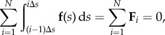
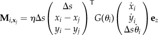
In this section, we describe the asymptotic coarse-graining formulation by integrating the moment balance system (2.1)–(2.2). The aim of this formulation is to bypass the complexity arising from the unknown contact forces (2.3), not defined constitutively, thus requiring the Lagrange multiplier τ to ensure inextensibility (2.7). Integrating the balance of contact forces over the whole filament (2.1), we get

where external contact forces are given by n(L) = n(0) = 0. The filament is conveniently divided in N rod-like segments with Δs = L/N. In the asymptotic limit of a small non-zero Δs, the filament can be coarse-grained via a semi-Riemann sum

3.1

so that F_i represents the total contact force experienced by the ith element. For a filament free from external torques, m(L) = m(0) = 0, the total moment balance (2.2) simply reads

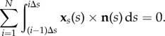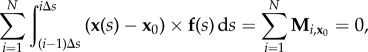
After partial integration, and exploiting the force balance (2.1), we find

3.2

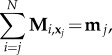
which is independent of n(s). Similarly, M_i,x0 is the ith moment about x₀ = x(0). As required, the total moment balance above is independent of the bending moment. Integration by parts of (2.2) for the jth element instead introduces the effect of the elastic bending moments via

3.3

where m_j = m((j − 1)L/N) and . Here, it is convenient to write the moment M_i,xj relative to x_j, whilst m_j is the bending moment contribution from the jth element and, as previously, it is linearly related to the curvature m(s) = E_bθ_se_z. Distinct finite difference approximations may be employed for θ_s [4,11,33]. For simplicity, we use the backward difference formula

3.4

where κ = E_b/Δs. The contact force f(s) in (3.1)–(3.3) is given by the hydrodynamic coupling (2.4).

We introduce now the geometry of deformation for centreline x(s, t) for the the coarse-grained elastohydrodynamic system. It is convenient to describe filament centreline in terms of the tangent angle θ (figure 1), where 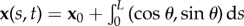, so that in the coarse-graining limit, we have

3.5

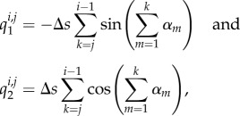
for i = 1, …, N, thus x_i = x((i − 1)L/N) = (x_i, y_i), where θ_k is the angle between e_x and e_k,∥ of the kth element, e_k,∥ = (cosθ_k, sinθ_k), e_k,⊥ = (−sinθ_k, cosθ_k), thus ensuring inextensibility intrinsically. Owing to the curvature dependence in (3.3), it is simpler to define the tangent angle in terms of the backward difference angle, α_i = θ_i − θ_i−1, i.e. the angle between e_i−1,∥ and e_i,∥,

3.6

by setting α₁ = θ₁. This reduces the filament centreline x(s, t) to only N + 2 parameters (x₀, y₀, α₁, …, α_N) (see [29]). The total force balance (3.1) and torque balance (3.2), together with N − 1 equations for the internal moment balance (3.3), further closes the elastohydrodynamic system with N + 2 scalar equations.

The resistive force theory approximation (2.4) allows for further analytical progress, as described in the seminal work by Gray & Hancock [46], by expressing the anisotropic operator in terms of tangent angle. Thus F_i and M_i,xj can be integrated analytically over the coarse-grained elements and expressed in terms of , where the overdots represent time derivatives. For simplicity, we assume linear interpolation of the shape function along the length s of each coarse-grained element. Thus from (3.5) the velocity of the centreline can be expressed as

At the fixed frame of reference, the contact forces over the ith coarse-element read [30,47]

3.7

where

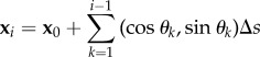
Similarly, the contact moment at the ith element relative to x_j takes the form

3.8

with

3.9

where the above set of 3N variables X_3N = (x₁, …, x_N, y₁, …, y_N, θ₁, …, θ_N) can be reduced to N + 2 variables X = (x₁, y₁, θ₁, …, α_N) via X_3N = QX, as described in detail in appendix A. The coarse-grained elastohydrodynamics (3.1)–(3.8) reduces to a non-dimensional system of ordinary differential equations

3.10

where Sp is the ‘sperm number’ as defined in (2.5), following the same recalling used for the classical system in §2. The general forms of the matrices A and B are also defined in appendix A.

4. Comparison between the classical and coarse-grained formulations

The classical elastohydrodynamic system is solved using the numerical scheme used in [11,35,52], briefly described here for comparison purpose. The system (2.5)–(2.7) couples nonlinearly a fourth-order PDE with a second-order BVP for the unknown line tension, yielding severe constraints for the time-stepping size if all terms are treated explicitly [11,52]. This is resolved by employing a second-order implicit–explicit method (IMEX) [53], where only the higher-order terms are treated implicitly, and before any previous time level is available, the second-order IMEX is replaced by the first-order IMEX [53]. The arclength discretization is uniform with N intervals, while second-order divided differences are used to approximate spatial derivatives, in which skew operators are applied at the boundaries [11,52]. The timestep thus can be chosen to be the same order of magnitude as the grid spacing, yielding a first-order constraint for time-stepping. Each iteration is made in two steps: first, the BVP for the Lagrange multiplier τ, equation (2.7), is solved for a given filament configuration x at time t_n, from which equation (2.5) can be timestepped to obtain new filament configuration x at t_n+1. Theoretical and empirical validation of this scheme is provided in [11,35,52].

The coarse-grained elastohydrodynamic system (3.10) does not require evaluation of Lagrange multipliers. The inextensibility is satisfied by model construction, while the asymptotic coarse-graining allows for a straightforward semi-analytic relation between the filament kinematics and the elastohydrodynamic forces and torques. The ordinary differential equation (ODE) system (3.10) is straightforward to implement using any solver or numerical scheme of choice. To illustrate this, we solved (3.10) using the built-in ode15s Matlab solver, which uses a variable-order, variable-step method based on the numerical differentiation formulae of orders 1 to 5 [54]. All computations for both the classical and coarse-grained formulation were conducted on an Intel Core i5-6500 processor, 3.20 GHz, using Matlab software.

In what follows, we study the transient dynamics of a filament decaying from an initial configuration [20,38,55], set to be a half-circle and a parabola. The filament thus unbends to its straight equilibrium configuration. Figure 2 contrasts the coarse-grained filament configuration and difference angle α for N = 5 and N = 50. A remarkable agreement between the dynamics of a very coarse filament (with only five segments) and N = 50 is observed. Indeed, the bulk-part elastohydrodynamics is well captured by the the coarser system. This is despite the shape inaccuracies associated with high curvatures. The shape discrepancies are continuously reduced as the filament approaches the equilibrium state. A higher number of segments smoothes the elastohydrodynamic hyperdiffusion profile, thus acting as an effective spatial spline interpolation for each filament configuration in time (compare the angle plots in figure 2). De facto, the coarse-grained system is able to capture the filament elastohydrodynamics with excellent accuracy even for very coarse filaments when compared with the classical system. This is in agreement with figure 3 which depicts the discrepancy between the classical, x_c, and the coarse-grained, x_cg, solutions via

so that D_max = 0 if the agreement is exact [4]. For D_max ≈ 0.1 or less, the agreement is observed to be very good, as illustrated by the shapes for an increasing N (figure 3). For D_max < 0.05 the difference between the classical and coarse-grained solutions is almost undistinguishable; see for example the detailed insets in figure 3b,c on the right column. D_max decays approximately with 1/N in figure 3, as expected from linear interpolation of curves. The dynamics is thus weakly influenced by the coarse-graining refinement level of the system. This feature may be exploited to reduce the dimensionality of the linear system while keeping a reasonable accuracy of the dynamics. By construction the asymptotic integrals along coarse-grained segments will tend to zero for infinitesimal Δs, as detailed in equations (3.1) and (3.2). This introduces a higher bound for N. For N > 80, or equivalently for Δs/L < 1%, the system becomes numerically stiff and requires an excessive time-stepping refinement.

Figure 2.

Relaxation dynamics of a filament from a half-circle configuration with five elements (dotted line) and 50 elements (continuous line) and Sp = 4. The filaments are drawn on the left plot at t = 0 (dark blue) and at regular time increment of 0.2. The colour maps on the right show the spatio-temporal transient dynamics of the angle α_i = θ_i − θ_i−1 between consecutive elements, i.e. the discrete curvature. The colour map above (below) corresponds to the coarse-grained filament with N = 5 (N = 50) elements. Note that the values of α are smaller for the finer case, as refinement induces a smoother spatio-temporal map, hence smaller angle difference between segments.

Figure 3.

Comparison between the classical and the coarse-grained systems for increasing N. A fine discretization for the classical solution is fixed for all cases. (a–c) Comparison of the classical (red) and the coarse-grained (black) for N = 10, 30, 75, as indicated on the D_max plot. The right-hand column exposes the detailed shape of small parts of the filaments, indicated by the small grey rectangles. The good accuracy of the coarse-grained solution is observed even for very small number of segments N.

We further compare the computational time of both formulations in table 1. We focus on the numerically stiff regime of the classical system, occurring at low sperm number Sp, for effectively stiff filaments, and high curvatures. N = 70 was used for all simulations of the coarse-grained model. The classical system, however, requires distinct spatio-temporal discretizations according to total length error associated to each parameter regime [11], chosen to give the smallest computing time. Table 1 shows that the coarse-grained model has a maximum time duration of 3 s for Sp = 2. The computational time for the coarse-grained system increases as Sp is reduced, although the accretion is marginal. On the other hand, the classical system suffers dramatically from numerical stiffness. For the lowest length-error tolerance imposed, 1%, the computational time increases by a factor of 74 for the half-circle case when Sp is reduced. The time required for the parabola is of the order of hours. The latter is exacerbated when length-error tolerance is reduced to 0.01%. In this case, even for Sp = 4, the computational time surpasses one hour to solve the parabola initial shape. De facto, this regime is known to be numerically challenging, as one approaches the limit of validity of the resistive-force theory. Elastic forces and torques are very large compared to the viscous dissipation, characterized by a snap-through, fast unbending of the filament towards the relaxation state, thus requiring very fine time-stepping to resolve this fast transient phase. Table 1 demonstrates how the coarse-grained approach outperforms the classical elastohydrodynamic system.

Table 1.

Computing times in seconds for the two relaxation tests and two different sperm numbers. Tolerance of the length error only applies to the classical system.

	coarse-grained	tolerance	classical
test	system N = 70	length error	system
Sp = 4
half-circle		1%	1.3
	2	0.1%	249
		0.01%	3750
parabola		1%	90
	1.5	0.1%	1820
		0.01%	>1 h
Sp = 2
half-circle		1%	97
	3	0.1%	850
		0.01%	>1 h
parabola		1%	>1 h
	1.7	0.1%	>1 h
		0.01%	>1 h

5. Bio-applications

In this section, we apply the coarse-grained formulation for a variety of elastohydrodynamic systems and boundary conditions found in biology, emphasizing the simplicity and robustness of this approach. We focus on the filament buckling problem (§5.1), well known for its numerical stiffness, instability and challenges associated with boundary forces. We also study the magnetic actuation of swimming filament (§5.2) and the dynamics of cross-linked filament bundles and flagella (§5.3), including explicit elastic coupling among coarse-grained filaments. Other interactions, via boundary forces/torques or their distribution along the filament, such as in gravitational and electromagnetic effects, as well as background flows, may be accounted effortlessly within this formulation.

5.1. Filament buckling instability

The coarse-grained system equation (3.10) is particularly suitable for non-trivial boundary constraints, such as in fixed or moving boundary cases. In such situations, either the position (angle) or the force (torque) is imposed at the extremities. Here, we consider an initially straight filament with the proximal end, s = 0, pinned, so that the position is fixed but free from external torques. The distal boundary, s = 1, moves with an imposed velocity towards the proximal end, although free from external torques. Post-transient dynamics, at the steady state, leads to the celebrated Euler-elastica BVP which admits exact solutions in terms of elliptic functions [1,51]. In this limit, contact forces balance exactly the imposed load, and the shape is defined by the torque balance [1,51]. The transient dynamics of a filament buckling in a viscous fluid, however, depends on the distribution of both contact forces and torques that evolves in time. This requires the evaluation of unknown boundary forces at the proximal end, s = 0, while the distal end, s = 1, follows prescribed kinematics. We consider that the two endpoints are driven towards each other at a constant speed. This is a non-trivial task within the classical elastohydrodynamic formulation, as the usual separation between equations (2.5) and (2.7) for the customary free force/torque condition is not possible. Instead, the unknown tension line at the boundary, required for the inextensibility constraint, is nonlinearly coupled with the hyperdiffusive elastohydrodynamics (2.5). This difficulty is augmented by the fact that the buckling instability is instigated by excessive compressive force distribution to a critical level in which the filament cannot uphold and buckles. This occurs via a pitchfork bifurcation with equal chances to buckle in either direction, as is also a solution [51]. The initial straight configuration thus requires an infinitesimal bias to trigger the unstable modes dynamically.

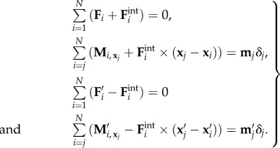
The buckling phenomenon is however straightforward within the coarse-grained framework. For this, we introduce unknown contact forces, respectively, for the proximal and distal ends P₀ and P_N, and associated moments in the coarse-grained system equation (3.10), which reduces to

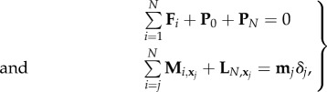5.1

for j = 1, …, N, where δ_j is defined as δ₁ = 0 and δ_j≠1 = 1, and L_N,xi is the moment induced by P_N with respect to the point x_i, L_N,xi = (x_N+1 − x_i) × P_N. The unknown forces are supplemented by the kinematic constraints and , where k is positive. The detailed form of the linear system may be found in appendix A.3.

Figure 4 depicts the shape evolution for the first three initially unstable modes at the onset of the instability and beyond, for Sp = 2, 4, 8 from equation (5.1). They capture the fast transient solutions for an effectively stiff filament, Sp = 2 (also the numerically stiff case), which rapidly collapses into the static, steady-state Euler-elastica solutions for the first two modes, top and middle plots in figure 4 for Sp = 2. Complex mode competition is easily accessible. This is demonstrated by the third mode dynamics (bottom row). The coarse-grained system thus unveils the cascade of unstable modes towards the stable shape; see third mode for Sp = 8. For Sp = 2, these transitions occur via fast distal–proximal travelling waves, with distinct wave duration and speed, as demonstrated by the spatio-temporal-α profiles. As Sp increases, more unstable modes are instigated, giving rise to a wide diversity of nonlinear phenomena and interactions among the participating modes, in particular mode-coupling competition; see for example Sp = 4, 8 in figure 4. Investigation of mode stability at advanced, nonlinear stages is also possible using this formulation, for instance, by studying the energy landscape and bifurcation diagrams. Despite the current gap in the literature, detailed nonlinear investigation of the buckling phenomenon in a viscous environment is outside the scope of the present paper and will be explored elsewhere.

Figure 4.

Visualization of the buckling phenomenon for three different sperm numbers. Here N = 36 and k = 1.5. The filament is displayed at regular intervals of time, coloured from blue (beginning) to red (end). Three different initial conditions lead to different outcomes. The colour map graphs show time on the x-axis and link number (discrete arclength) on the y-axis. The colours show the curvature (angles) over time, from blue for a highly negative curvature to red for a highly positive one. The filament quickly takes a waveform with fewer waves as time goes on. The higher the sperm number is, the longer it takes for the waves to vanish (note that the total time on the graphs is longer as the sperm number increases).

5.2. Magnetic swimmer

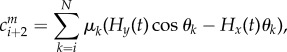
Following recent resurgence of interest in magnetically driven elastic fibres for the purpose of locomotion at micro- or macro-scale [49,56,57], we solve the coarse-graining of a magnetic filament under the influence of an external magnetic field. In this section, we consider a filament magnetized with a homogeneous magnetic moment μ along its arclength, directed towards the tangential direction, under the action of a uniform, time-varying sinusoidal oscillatory magnetic field H(t). The new terms arising from external torques are thus straightforward, as it only requires the addition of a distribution of the magnetic moments in equation (3.10), m^m_i = μ_ie_i,∥ × H, and reads

5.2

Figure 5 shows an example of a partially magnetized swimmer moving according to the applied sinusoidal magnetic field, with N = 20 and Sp = 4, starting from a straight configuration for approximately five cycles. The coarse-grained system is numerically cheap, as it has a reduced number of mesh points. Thus it allows for optimization studies involving the continuous evaluation of objective function across a large parameter space. Previous studies demonstrated that the classical system leads to very expensive numerical simulations [35,49], making any parameter search very challenging. This opens new possibilities for investigations within control theory, as well as optimal control [47,58] by using this approach.

Figure 5.

Example of magnetic drive with a sinusoidal orthogonal magnetic field. One-quarter of the length of the filament (i.e. the first five elements) is not magnetized, and the other part is constantly magnetized. Here Sp = 4, N = 20, M = 1, H(t) = cos(t)e_y/15. (a) The filament is displayed at regular intervals of time over a time period, coloured from blue (beginning) to red (end). (b) The red line shows the position of the filament at the end of the simulation. The thin dotted and thick blue lines, respectively, show the trajectory of the non-magnetized end and the centroid of the filament.

5.3. Cross-linked filament bundles and flagella

In this section, we focus on biological systems involving time-dependent load distributions. This could arise, for example, via mechano-sensory coupling in biological structures and biochemical landscapes. Flagella and cilia found in eukaryotes are perfect exemplars of the latter [59]. They are composed by a geometrical arrangement of semi-flexible filaments interconnected by elastic linking proteins, called axoneme [60]. Its generic form is composed by 9 + 2 microtubule doublets surrounding a central pair [50,61,62], observed in both motile and non-motile form. Flagella are a challenging mathematical system. It couples nanometric scales from the molecular motor biochemical activation with microscopic properties of the elastic structure, as observed for the purpose of spermatozoa transport [59,63]. A geometrical abstraction of this system based on the sliding filament mechanism was first proposed by Brokaw [64]. In the static case, for steady-state deformations, flagella are prone to the so-called counterbend phenomenon [50,61]. This occurs when distant parts of a passive flagellum (in absence of motor activity) bend in opposition to an imposed curvature elsewhere along the flagellum, for example, using the tip of a micropipette [62,65,66]. Theoretical models encoding the mean cross-linked filament-bundle mechanics were able to recover the counterbend phenomenon [50,51], from which material parameters could be measured directly from the resulting counter-curvature. The dynamics of passive flagellar bundles have been investigated using linear theory [50], and prediction of counter-travelling waves instigated by the non-local cross-linking moments reported. To date, a geometrically exact investigation is still lacking in the literature.

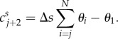
We consider the geometrically exact cross-linked filament bundle system for a passive bundle, that is a flagellum without molecular motor actuation, using the coarse-grained formulation. The sliding filament model [20,64] is particularly cumbersome within the classical elastohydrodynamic framework [52]. The boundary conditions are non-local due to the accumulative dependence of sliding moments along the bundle, and generally unknown during the dynamics. This becomes even more challenging when the bundle is driven via the molecular motor activity [20,67]. The coarse-grained formulation breaks the contribution of the sliding filament moments for each segment simply as

5.3

this last sum being a discretization of the sliding displacement integrated along the part of the filament going from jΔs to L, and κ^s an effective resistance to sliding between the sliding filaments [20]. The balance of forces and moments then reads

5.4

and describes an effective sliding filament bundle free from forces/torques at endpoints. We consider instead that the bundle is fixed and angularly actuated at the proximal end. Thus the first three equations in equation (5.4) are replaced with the kinematic conditions and for an angular amplitude a. Numerical solutions of the the coarse-graining system for a filament bundle angularly actuated at s = 0 with amplitude a = 0.4362 rad and κ^sΔs/κ = 0.06 are shown in figure 6. They confirm analytical prediction of counter-wave phenomenon from linear theory reported in [20, fig. 2], where waves are instigated non-locally, and travel in opposition to the imposed angular oscillation. The wavespeed and amplitudes involved depend on the cross-linking elastohydrodynamic parameters and the sperm number; compare Sp = 7 and Sp = 15 in figure 6. It is worth noting that coarse-graining system in equation (5.4) allows for straightforward generalization to include different motor-control hypotheses—central for the current flagella and cilia self-organization debate [20,67,68].

Figure 6.

Simulation of the counterbend phenomenon for two different sperm numbers (parameters are chosen in order to match those used in [20]: κ^sΔs/κ = 0.06, a = 0.4362 rad; and N = 50). The top row shows the behaviour of an actuated filament when no sliding resistance is added. The right column shows the same oscillation applied to the bundle model. For each case, the filament is displayed at regular intervals of time over a time period, coloured from blue (beginning) to red (end). The colour plots show the curvature (angles α) with respect to the time in x and the arclength in y. The travelling curvature wave generated by the actuation is visible at the bottom of all of the colour plots. For the counterbend case, a second travelling wave appears at the free end of the filament in the bundle case (bottom row).

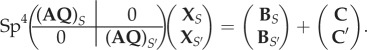
Finally, we consider the dynamics of two individual filaments embedded in a viscous fluid and coupled elastically via Hookean elastic springs (figure 7). The system thus involves the geometrically nonlinear elastohydrodynamics of two interacting elastic fibres. Once again, the classical elastohydrodynamic formulation is ill-posed. The discrete distribution of elastic springs introduces unknown point forces via equations (2.5) and (2.7) for each filament. We consider that the two-filament assembly is angularly actuated at one end (figure 7). We assume that the connecting elastic springs have an effective spring constant K connecting opposite nodes between the two filaments, placed at each coarse-grained segment junction for simplicity (figure 7). The equilibrium bundle diameter is d₀ at rest. The elastic force F^int_i exerted by the ith spring on the filament S (top filament) reads

where primes refer to the second filament. The coarse-grained formulation for S and S′ is thus augmented by the elastic reactions from each connecting spring, and their associated moments along each filament. Hence, the coupled system for the filaments S and S′ reads, respectively,

5.5

The proximal end of both constituent filaments is fixed, but the angle at s = 0 of the filament S (top filament) is actuated via θ₁(t) = a sin t. The filament S′ (bottom filament) is free from external actuation, thus its movement solely arises via the elastic coupling between them. A detailed description of the resulting two-filament system is provided in appendix A.5.

Figure 7.

Coupling between two filaments obtained with the coarse-grained approach. Here Sp = 4, a = 0.88 rad, . On the top, the actuated filament is represented at regular intervals of time over half a time period, coloured from blue (beginning) to red (end). The three colour maps display three parameters with respect to time and arclength: the angle α of the centreline (left), the distance d between the two filaments (middle) and the distance Δ between two facing nodes, normalized by their resting length d₀. Note that the beginning time for the graphs has been chosen big enough to skip transient phase and display only steady state. A travelling wave of curvature generated by the actuation of the top filament is visible in graph at the bottom left. The graph at the bottom in the middle shows the distance between the two filaments. Moreover, the graph at the bottom right captures the sliding distance between the two filaments.

Figure 7 shows numerical simulations for time evolution of the two-filament assembly, demonstrating the effectiveness of the connecting springs while transmitting bending moment from the top filament to the bottom one. A synchronous travelling wave of curvature is observed; see for example the tangent angle α of the centreline of the filament-pair in figure 7. The axial diameter d however evolves asymmetrically (middle plot in figure 7). The angular actuation of the top filament modifies the diametral distance between the filaments near the base, in an oscillatory motion, from where axial waves are propagated down the structure. Axial extensional waves (light yellow regions) propagate more easily than compressional waves in the axial direction (light green regions). The resulting sliding displacement Δ between the filament-pair is also depicted in the right graph in figure 7. Similarly to the radial distance, the relative sliding motion is concentrated towards the basal end; however, it is not propagated along the filament-pair. This is despite the fact that both filaments are inextensible, and tangential motion is easily propagated. Conversion of curvature into relative sliding motion between the filaments is not observed nor the counterbend phenomenon observed in figure 6; see the light yellow region for Δ ≈ 0 in figure 7. This suggests that simple elastic connectors between filaments are not effective while transmitting sliding moments. Instead, axial distortions are prevailed and propagated along the filament-pair assembly. The connecting springs contribute to forces along its direction, but mostly in the radial direction, perpendicular to centreline. The elastic springs are hinged at each connecting node, thus the constituent filaments are free from bending moments arising from the interfilament sliding (in contrast with figure 6). This supports the so-called geometric clutch mechanism proposed by Lindemann [69], where axial displacements are central for flagellar mechanics. These results further show that the sliding filament mechanism present in flagellar systems [50,61,64] is far more complex than this simplistic two-filament cross-linked assembly [5,20,64,68,70].

6. Conclusion

This paper studies inertialess fluid–structure interaction of inextensible filaments commonly found in biological systems. The nonlinear coupling between the geometry of deformation and the physical effects invariably results in intricate governing equations that negotiate elastohydrodynamical interactions with non-holonomic constraints, as a direct consequence of the filament inextensibility. As a result, the classical elastohydrodynamical formulation is prone to numerical instabilities, requires penalization methods and high-order spatio-temporal propagators. Here, we exploit the momentum balance in the asymptotic limit of small rod-like elements, from which the system can be integrated semi-analytically. This bypasses the bottleneck associated with the inextensibilty constraint, and does not require the use of Lagrange multipliers to solve the system. We further show the equivalence between the two formalisms, as well as a direct comparison between their numerical performances. The coarse-graining formalism was shown to outperform the classical approach, in particular for numerically stiff regimes where the classical system performs poorly. The coarse-graining structure also allowed faster computations, more than a hundred times faster than previous implementations. The coarse-graining approach is simple and intuitive to implement, and generalizations for complex interaction of multiple rods, active filaments, flagella, Brownian polymer dynamics and non-local hydrodynamics are straightforward.

We employed the coarse-grained formulation to study distinct biologically inspired systems: the buckling instability of bio-filaments, the magnetic actuation of a micro-swimmer and the dynamics of cross-linked filament bundles and flagella. With the exception of the magnetic swimmer case, the results obtained here for the other systems are new in the literature. For the buckling problem, travelling waves are generated and propagated with different speeds, depending on the elastohydrodynamic properties of the filament and its interaction with other competing modes, figure 4; thus relevant to biological systems in which buckling is a naturally occurring phenomenon [6]. The coarse-graining approach successfully captured the counterbend phenomenon in cross-linked filament bundles [20,50], figure 6, including geometrical nonlinearities. Finally, motivated by mathematical abstractions of flagellar systems [5,68], we solved the dynamics of interactions between two individual filaments interconnected with elastic springs. Numerical simulations indicated that the sliding between the filaments is not instigated by changes in curvature, as assumed by the sliding-filament mechanism [64]. Instead, axial distortions are propagated along the two-filament assembly, in agreement with the geometric clutch hypothesis [69]. These modes of deformation are central for the molecular-motor control debate in flagellar systems [20,68].

The results presented here offer new possibilities for theoretical investigations, for instance, of the elastohydrodynamic self-organization of fibres, many interacting filaments, cytoskeleton modelling, manoeuvrability of micro-magnetic robots [47,58], as well as optimal strategy of deformation for micro-locomotion [71]. Only basic knowledge of systems of linear equations is required and implementation achieved with any solver of choice. We hope that the simplicity of the formalism, the numerical robustness and easy-to-implement generalizations will appeal to the biology, soft-matter and interdisciplinary communities at large.

Appendix A

A.1. Parametrization in the coarse-graining model

In the asymptotic description, the filament can be described with two different sets of parameters (figure 1).

• —The N + 2 parameters X = (x₁, y₁, θ₁, α₂, …, α_N).
• —The 3N parameters X_3N = (x₁, …, x_N, y₁, …, y_N, θ₁, …, θ_N).

The second set uses 3N parameters where N + 2 are sufficient. Going from to can be done via the following transformation matrices:

with

and

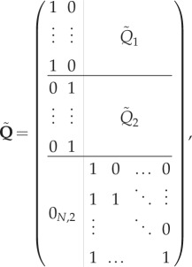A 1

where and are N × N matrices whose elements are given by the general formula

with q^i,j₁ = q^i,j₂ = 0 if i ≥ j. The tildes refer to the dimensional quantities.

A.2. Matricial form of the ordinary differential equation system

Using the explicit expressions of the different contributions (3.4), (3.7) and (3.8), and after non-dimensionalizing, we can rewrite the system (3.1)–(3.3) in a matricial form:

A 2

where the terms are defined as follows:

• —
  The matrix A is a (N + 2) × 3N matrix whose coefficients are given, for all i in {1, …, N} and j in {i, …, N}, by

  

  where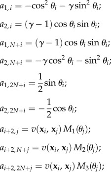

  

  and M₁, M₂, M₃ are the columns of the matrix (3.9). If j < i, then a_i+2,j = a_i+2,N+j = a_i+2,2N+j = 0.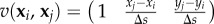
• —Q is the non-dimensionalized version of the transformation matrix (A 1). It is defined by replacing and with and in the expression of .
• —
  B is a column vector of size N + 2, given by

  

A.3. Buckling instability system

The buckling problem requires two unknown contact forces P₀ and P_N (see §5.1). This yields four additional unknowns: P_0x, P_0y, P_Nx, P_Ny. We add four equations to the system (3.10) by embedding the buckling kinematic constraints and 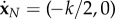, where k is positive. The new system of (N + 6) scalar equations is given by

A 3

where

A 4

and

A 5

where matrices A, B and Q are defined as in appendix A.2.

A.4. Magnetic swimmer

The matricial system describing a magnetically driven filament with the coarse-graining approach reads

A 6

It is simply obtained by adding to the system (3.10), the magnetic effect vector C^m = (c^m₁ … c^m_N+2)^T, with c^m₁ = c^m₂ = 0 and ∀i ∈{1, …, N},

where H_x(t) and H_y(t) are the components of the magnetic field along the x- and y-axis.

A.5. Cross-linked filament bundle

The system (5.5) describing a filament bundle with sliding resistance takes the following matricial form:

A 7

with C^s = (c^s₁ … c^s_N+2)^T, with c^s₁ = c^s₂ = 0 and ∀j ∈{1, …, N},

In the case of two interacting filaments, S and S′, the new coupled dimensionless system of (2N + 4) equations reads

A 8

In the above, A, B, Q and X are defined as previously, where the subscripts denote the filament S or S′. The interaction vectors C and C′ are defined as follows:

A 9

The above system describes a bundle with free endpoints. However, in the case studied in equation (A 8), both filaments have a fixed proximal end, and the filament S is actuated at its proximal end (prescribed angle θ₁). We embed these boundary conditions in the system by replacing the first three lines with the constraints , , , and its N + 3th and N + 4th equations (i.e. the first two equations for the second filament) by the constraint equations and .

Data accessibility

The Matlab codes used to run the simulations presented in this paper are available on github via this link: https://github.com/Clementmoreau/Filament.

Authors contributions

C.M. conducted the research, wrote the paper and performed the numerical simulations. L.G. designed and conducted the research, and wrote the paper. H.G. designed and conducted the research, and wrote the paper.

Competing interests

We declare we have no competing interests.

Funding

The authors were partially funded by the CNRS through the project Défi InFIniti-AAP 2017.

References

- 1.Antman SS. 2005. Nonlinear problems of elasticity. Applied Mathematical Sciences, vol. 107 Berlin, Germany: Springer. [Google Scholar]
- 2.Alberts B. 2002. Molecular biology of the cell. New York, NY: Garland Science. [Google Scholar]
- 3.Howard J. 2001. Mechanics of motor proteins and the cytoskeleton. Sunderland, MA: Sinauer Associates. [Google Scholar]
- 4.Gadêlha H, Gaffney EA, Smith DJ, Kirkman-Brown JC. 2010. Nonlinear instability in flagellar dynamics: a novel modulation mechanism in sperm migration? J. R. Soc. Interface 7, 1689–1697. ( 10.1098/rsif.2010.0136) [DOI] [PMC free article] [PubMed] [Google Scholar]
- 5.Camalet S, Jülicher F, Prost J. 1999. Self-organized beating and swimming of internally driven filaments. Phys. Rev. Lett. 82, 1590–1593. ( 10.1103/PhysRevLett.82.1590) [DOI] [Google Scholar]
- 6.Bourdieu L, Duke T, Elowitz MB, Winkelmann DA, Leibler S, Libchaber A. 1995. Spiral defects in motility assays: a measure of motor protein force. Phys. Rev. Lett. 75, 176–179. ( 10.1103/PhysRevLett.75.176) [DOI] [PubMed] [Google Scholar]
- 7.Goldstein RE, Langer SA. 1995. Nonlinear dynamics of stiff polymers. Phys. Rev. Lett. 75, 1094–1097. ( 10.1103/PhysRevLett.75.1094) [DOI] [PubMed] [Google Scholar]
- 8.Fu HC, Wolgemuth CW, Powers TR. 2008. Beating patterns of filaments in viscoelastic fluids. Phys. Rev. E 78, 041913 ( 10.1103/PhysRevE.78.041913) [DOI] [PubMed] [Google Scholar]
- 9.Yu TS, Lauga E, Hosoi AE. 2006. Experimental investigations of elastic tail propulsion at low reynolds number. Phys. Fluids 18, 0917011 ( 10.1063/1.2349585) [DOI] [Google Scholar]
- 10.Olson SD, Lim S, Cortez R. 2013. Modeling the dynamics of an elastic rod with intrinsic curvature and twist using a regularized Stokes formulation. J. Comput. Phys. 238, 169–187. ( 10.1016/j.jcp.2012.12.026) [DOI] [Google Scholar]
- 11.Tornberg AK, Shelley MJ. 2004. Simulating the dynamics and interactions of flexible fibers in Stokes flows. J. Comput. Phys. 196, 8–40. ( 10.1016/j.jcp.2003.10.017) [DOI] [Google Scholar]
- 12.Kantsler V, Goldstein RE. 2012. Fluctuations, dynamics, and the stretch-coil transition of single actin filaments in extensional flows. Phys. Rev. Lett. 108, 038103 ( 10.1103/PhysRevLett.108.038103) [DOI] [PubMed] [Google Scholar]
- 13.Sanchez T, Chen DTN, DeCamp SJ, Heymann M, Dogic Z. 2012. Spontaneous motion in hierarchically assembled active matter. Nature 491, 431–434. ( 10.1038/nature11591) [DOI] [PMC free article] [PubMed] [Google Scholar]
- 14.Brangwynne CP, MacKintosh FC, Kumar S, Geisse NA, Talbot J, Mahadevan L, Parker KK, Ingber DE, Weitz DA. 2006. Microtubules can bear enhanced compressive loads in living cells because of lateral reinforcement. J. Cell Biol. 173, 733–741. ( 10.1083/jcb.200601060) [DOI] [PMC free article] [PubMed] [Google Scholar]
- 15.Plouraboue F, Thiam I, Delmotte B, Climent E. 2017. Identification of internal properties of fibers and micro-swimmers. Proc. R. Soc. A 473, 20160517 ( 10.1098/rspa.2016.0517) [DOI] [PMC free article] [PubMed] [Google Scholar]
- 16.Heussinger C, Schüller F, Frey E. 2010. Statics and dynamics of the wormlike bundle model. Phys. Rev. E 81, 021904 ( 10.1103/PhysRevE.81.021904) [DOI] [PubMed] [Google Scholar]
- 17.E. Claessens MMA, Semmrich C, Ramos L, Bausch AR. 2008. Helical twist controls the thickness of f-actin bundles. Proc. Natl Acad. Sci. USA 105, 8819–8822. ( 10.1073/pnas.0711149105) [DOI] [PMC free article] [PubMed] [Google Scholar]
- 18.Claessens MMAE, Bathe M, Frey E, Bausch AR. 2006. Actin-binding proteins sensitively mediate f-actin bundle stiffness. Nat. Mater. 5, 748–753. ( 10.1038/nmat1718) [DOI] [PubMed] [Google Scholar]
- 19.Hines M, Blum JJ. 1979. Bend propagation in flagella. II. Incorporation of dynein cross-bridge kinetics into the equations of motion. Biophys. J. 25, 421–441. ( 10.1016/S0006-3495(79)85313-8) [DOI] [PMC free article] [PubMed] [Google Scholar]
- 20.Coy R, Gadêlha H. 2017. The counterbend dynamics of cross-linked filament bundles and flagella. J. R. Soc. Interface 14, 20170065 ( 10.1098/rsif.2017.0065) [DOI] [PMC free article] [PubMed] [Google Scholar]
- 21.Schoeller SF, Keaveny EE. 2018. From flagellar undulations to collective motion: predicting the dynamics of sperm suspensions. J. R. Soc. Interface 15, 20170834 ( 10.1098/rsif.2017.0834) [DOI] [PMC free article] [PubMed] [Google Scholar]
- 22.Lauga E, Powers TR. 2009. The hydrodynamics of swimming microorganisms. Rep. Prog. Phys. 72, 096601 ( 10.1088/0034-4885/72/9/096601) [DOI] [Google Scholar]
- 23.Purcell EM. 1977. Life at low Reynolds number. Am. J. Phys. 45, 3–11. ( 10.1119/1.10903) [DOI] [Google Scholar]
- 24.Hines M, Blum JJ. 1978. Bend propagation in flagella. I. Derivation of equations of motion and their simulation. Biophys. J. 23, 41–57. ( 10.1016/S0006-3495(78)85431-9) [DOI] [PMC free article] [PubMed] [Google Scholar]
- 25.Lauga E, Powers TR. 2009. The hydrodynamics of swimming microorganisms. Rep. Prog. Phys. 72, 096601 ( 10.1088/0034-4885/72/9/096601) [DOI] [Google Scholar]
- 26.Powers TR. 2010. Dynamics of filaments and membranes in a viscous fluid. Rev. Mod. Phys. 82, 1607–1631. ( 10.1103/RevModPhys.82.1607) [DOI] [Google Scholar]
- 27.Shelley MJ, Zhang J. 2011. Flapping and bending bodies interacting with fluid flows. Annu. Rev. Fluid Mech. 43, 449–465. ( 10.1146/annurev-fluid-121108-145456) [DOI] [Google Scholar]
- 28.Brennen C, Winet H. 1977. Fluid mechanics of propulsion by cilia and flagella. Annu. Rev. Fluid Mech. 9, 339–398. ( 10.1146/annurev.fl.09.010177.002011) [DOI] [Google Scholar]
- 29.Alouges F, DeSimone A, Giraldi L, Zoppello M. 2013. Self-propulsion of slender micro-swimmers by curvature control: N-link swimmers. Int. J. Non-Linear Mech. 56, 132–141. ( 10.1016/j.ijnonlinmec.2013.04.012) [DOI] [Google Scholar]
- 30.Alouges F, DeSimone A, Giraldi L, Zoppello M. 2015. Can magnetic multilayers propel artificial microswimmers mimicking sperm cells? Soft Robot. 2, 117–128. ( 10.1089/soro.2015.0007) [DOI] [Google Scholar]
- 31.Giraldi L, Martinon P, Zoppello M. 2013. Controllability and optimal strokes for N-link micro-swimmer. In Proc. 52nd IEEE Conf. on Decision and Control, Florence, Italy, 10–13 December 2013, pp. 3870–3875. ( 10.1109/CDC.2013.6760480) [DOI] [Google Scholar]
- 32.Giraldi L, Martinon P, Zoppello M. 2015. Optimal design of the three-link purcell swimmer. Phys. Rev. E 91, 023012 ( 10.1103/PhysRevE.91.023012) [DOI] [PubMed] [Google Scholar]
- 33.Delmotte B, Climent E, Plouraboué F. 2015. A general formulation of Bead Models applied to flexible fibers and active filaments at low Reynolds number. J. Comput. Phys. 286, 14–37. ( 10.1016/j.jcp.2015.01.026) [DOI] [Google Scholar]
- 34.CosentinoLagomarsino M, Pagonabarraga I, Lowe CP. 2005. Hydrodynamic induced deformation and orientation of a microscopic elastic filament. Phys. Rev. Lett. 94, 148104 ( 10.1103/PhysRevLett.94.148104) [DOI] [PubMed] [Google Scholar]
- 35.Montenegro-Johnson TD, Gadêlha H, Smith DJ. 2015. Spermatozoa scattering by a microchannel feature: an elastohydrodynamic model. R. Soc. open sci. 2, 140475 ( 10.1098/rsos.140475) [DOI] [PMC free article] [PubMed] [Google Scholar]
- 36.Brokaw CJ. 2014. Computer simulation of flagellar movement X: doublet pair splitting and bend propagation modeled using stochastic dynein kinetics. Cytoskeleton 71, 273–284. ( 10.1002/cm.21168) [DOI] [PubMed] [Google Scholar]
- 37.Johnson RE, Brokaw CJ. 1979. Flagellar hydrodynamics. Biophys. J. 25, 113–127. ( 10.1016/S0006-3495(79)85281-9) [DOI] [PMC free article] [PubMed] [Google Scholar]
- 38.Wiggins CH, Goldstein RE. 1998. Flexive and propulsive dynamics of elastica at low Reynolds number. Phys. Rev. Lett. 80, 3879–3882. ( 10.1103/PhysRevLett.80.3879) [DOI] [Google Scholar]
- 39.Klapper I. 1996. Biological applications of the dynamics of twisted elastic rods. J. Comput. Phys. 125, 325–337. ( 10.1006/jcph.1996.0097) [DOI] [Google Scholar]
- 40.Hou TY, Lowengrub JS, Shelley MJ. 1994. Removing the stiffness from interfacial flows with surface tension. J. Comput. Phys. 114, 312–338. ( 10.1006/jcph.1994.1170) [DOI] [Google Scholar]
- 41.Hou TY, Klapper I, Si H. 1998. Removing the stiffness of curvature in computing 3-D filaments. J. Comput. Phys. 143, 628–664. ( 10.1006/jcph.1998.5977) [DOI] [Google Scholar]
- 42.Rodrigues DS, Ausas RF, Mut F, Buscaglia GC. 2015. A semi-implicit finite element method for viscous lipid membranes. J. Comput. Phys. 298, 565–584. ( 10.1016/j.jcp.2015.06.010) [DOI] [Google Scholar]
- 43.Lowe CP. 2003. Dynamics of filaments: modelling the dynamics of driven microfilaments. Phil. Trans. R. Soc. Lond. B 358, 1543–1550. ( 10.1098/rstb.2003.1340) [DOI] [PMC free article] [PubMed] [Google Scholar]
- 44.Wiggins CH, Riveline D, Ott A, Goldstein RE. 1998. Trapping and wiggling: elastohydrodynamics of driven microfilaments. Biophys. J. 74, 1043–1060. ( 10.1016/S0006-3495(98)74029-9) [DOI] [PMC free article] [PubMed] [Google Scholar]
- 45.Young Y-N. 2009. Hydrodynamic interactions between two semiflexible inextensible filaments in Stokes flow. Phys. Rev. E 79, 046317 ( 10.1103/PhysRevE.79.046317) [DOI] [PubMed] [Google Scholar]
- 46.Gray J, Hancock J. 1955. The propulsion of sea-urchin spermatozoa. J. Exp. Biol. 32, 802–814. [Google Scholar]
- 47.Giraldi L, Pomet J-B. 2017. Local controllability of the two-link magneto-elastic micro-swimmer. IEEE Trans. Automat. Contr. 62, 2512–2518. ( 10.1109/TAC.2016.2600158) [DOI] [Google Scholar]
- 48.Gutman E, Or Y. 2014. Simple model of a planar undulating magnetic microswimmer. Phys. Rev. E 90, 013012 ( 10.1103/PhysRevE.90.013012) [DOI] [PubMed] [Google Scholar]
- 49.Gadêlha H. 2013. On the optimal shape of magnetic swimmers. Regular Chaotic Dyn. 18, 75–84. ( 10.1134/S156035471301005X) [DOI] [Google Scholar]
- 50.Gadêlha H, Gaffney EA, Goriely A. 2013. The counterbend phenomenon in flagellar axonemes and cross-linked filament bundles. Proc. Natl Acad Sci. USA 110, 12 180–12 185. ( 10.1073/pnas.1302113110) [DOI] [PMC free article] [PubMed] [Google Scholar]
- 51.Gadelha H. In press. The filament-bundle elastica. IMA J. Appl. Math. [Google Scholar]
- 52.Gadêlha H, Gaffney EA, Smith DJ, Kirkman-Brown JC. 2010. Nonlinear instability in flagellar dynamics: a novel modulation mechanism in sperm migration? J. R. Soc. Interface 7, 20100136 ( 10.1098/rsif.2010.0136) [DOI] [PMC free article] [PubMed] [Google Scholar]
- 53.Ascher UM, Ruuth SJ, Wetton BTR. 1995. Implicit-explicit methods for time-dependent partial differential equations. SIAM J. Numer. Anal. 32, 797–823. ( 10.1137/0732037) [DOI] [Google Scholar]
- 54.Shampine LF, Reichelt MW. 1997. The Matlab ODE suite. SIAM J. Sci. Comput. 18, 1–22. ( 10.1137/S1064827594276424) [DOI] [Google Scholar]
- 55.Wiggins CH, Riveline D, Ott A, Goldstein RE. 1998. Trapping and wiggling: elastohydrodynamics of driven microfilaments. Biophys. J. 74, 1043–1060. ( 10.1016/S0006-3495(98)74029-9) [DOI] [PMC free article] [PubMed] [Google Scholar]
- 56.Alouges F, DeSimone A, Giraldi L, Zoppello M. 2017. Purcell magneto-elastic swimmer controlled by external magnetic fields. IFAC-PapersOnLine 50, 4120–4125. ( 10.1016/j.ifacol.2017.08.798) [DOI] [Google Scholar]
- 57.Dreyfus R, Baudry J, Roper ML, Fermigier M, Stone HA, Bibette J. 2005. Microscopic artificial swimmers. Nature 437, 862–865. ( 10.1038/nature04090) [DOI] [PubMed] [Google Scholar]
- 58.Giraldi L, Moreau C, Lissy P, Pomet J-B. In press Addendum to ‘Local controllability of the two-link magneto-elastic micro-swimmer’. IEEE Trans. Automat. Contr. ( 10.1109/TAC.2017.2764422) [DOI] [Google Scholar]
- 59.Gaffney EA, Gadêlha H, Smith DJ, Blake JR, Kirkman-Brown JC. 2011. Mammalian sperm motility: observation and theory. Annu. Rev. Fluid Mech. 43, 501–528. ( 10.1146/annurev-fluid-121108-145442) [DOI] [Google Scholar]
- 60.Warner FD, Satir P. 1974. The structural basis of ciliary bend formation: radial spoke positional changes accompanying microtubule sliding. J. Cell Biol. 63, 35–63. ( 10.1083/jcb.63.1.35) [DOI] [PMC free article] [PubMed] [Google Scholar]
- 61.Lindemann CB, Macauley LJ, Lesich KA. 2005. The counterbend phenomenon in dynein-disabled rat sperm flagella and what it reveals about the interdoublet elasticity. Biophys. J. 89, 1165–1174. ( 10.1529/biophysj.105.060681) [DOI] [PMC free article] [PubMed] [Google Scholar]
- 62.Pelle DW, Brokaw CJ, Lesich KA, Lindemann CB. 2009. Mechanical properties of the passive sea urchin sperm flagellum. Cytoskeleton 66, 721–735. ( 10.1002/cm.20401) [DOI] [PubMed] [Google Scholar]
- 63.Ishimoto K, Gadêlha H, Gaffney EA, Smith DJ, Kirkman-Brown J. 2018. Human sperm swimming in a high viscosity mucus analogue. J. Theor. Biol. 446, 1–10. ( 10.1016/j.jtbi.2018.02.013) [DOI] [PubMed] [Google Scholar]
- 64.Brokaw CJ. 1972. Flagellar movement: a sliding filament model. Science 178, 455–462. ( 10.1126/science.178.4060.455) [DOI] [PubMed] [Google Scholar]
- 65.Lindemann CB, Macauley LJ, Lesich KA. 2005. The counterbend phenomenon in dynein-disabled rat sperm flagella and what it reveals about the interdoublet elasticity. Biophys. J. 89, 1165–1174. ( 10.1529/biophysj.105.060681) [DOI] [PMC free article] [PubMed] [Google Scholar]
- 66.Xu G, Wilson KS, Okamoto RJ, Shao J-Y, Dutcher SK, Bayly PV. 2016. Flexural rigidity and shear stiffness of flagella estimated from induced bends and counterbends. Biophys. J. 110, 2759–2768. ( 10.1016/j.bpj.2016.05.017) [DOI] [PMC free article] [PubMed] [Google Scholar]
- 67.Oriola D, Gadêlha H, Casademunt J. 2017. Nonlinear amplitude dynamics in flagellar beating. R. Soc. open sci. 4, 160698 ( 10.1098/rsos.160698) [DOI] [PMC free article] [PubMed] [Google Scholar]
- 68.Sartori P, Geyer VF, Scholich A, Jülicher F, Howard J. 2016. Dynamic curvature regulation accounts for the symmetric and asymmetric beats of Chlamydomonas flagella. eLife 5, e13258 ( 10.7554/eLife.13258) [DOI] [PMC free article] [PubMed] [Google Scholar]
- 69.Lindemann CB. 1994. A ‘geometric clutch’ hypothesis to explain oscillations of the axoneme of cilia and flagella. J. Theor. Biol. 168, 175–189. ( 10.1006/jtbi.1994.1097) [DOI] [Google Scholar]
- 70.Oriola D, Gadêlha H, Blanch-Mercader C, Casademunt J. 2014. Subharmonic oscillations of collective molecular motors. EPL (Europhys. Lett.) 107, 18002 ( 10.1209/0295-5075/107/18002) [DOI] [Google Scholar]
- 71.Wiezel O, Giraldi L, DeSimone A, Or Y, Alouges F. 2018 Energy-optimal small-amplitude strokes for multi-link microswimmers: Purcell's loops and Taylor's waves reconciled. ( http://arxiv.org/abs/1801.04687)
Associated Data
This section collects any data citations, data availability statements, or supplementary materials included in this article.
Supplementary Materials
Data Availability Statement