Unraveling the Differential Aggregation of Anionic and Nonionic Monorhamnolipids at Air–Water and Oil–Water Interfaces: A Classical Molecular Dynamics Simulation Study

Abstract

The molecular structure of a surfactant molecule is known to have a great effect on the interfacial properties. We employ molecular dynamics simulations for a detailed atomistic study of monolayers of the nonionic and anionic form of the most common congener of monorhamnolipids, α-rhamnopyranosyl-β-hydroxydecanoyl-β-hydroxydecanoate ((R,R)-Rha–C10-C10), at the air–water and oil–water interfaces. An atomistic-level understanding of monolayer aggregation is necessary to explain a recent experimental observation indicating that nonionic and anionic Rha–C10-C10 show surprisingly different surface area per molecule at the critical micelle concentration. Surface-pressure analysis, interface formation energy calculations, and mass density profiles of the monolayers at the air–water interface show similar properties between nonionic and anionic Rha–C10-C10 aggregation. It is found that there is a significant difference in the headgroup conformations of Rha–C10-C10 in the nonionic and anionic monolayers. Hydrogen bonding interactions between the Rha–C10-C10 molecules in the monolayers is also significantly different between nonionic and anionic forms. Representative snapshots of the simulated system at different surface concentrations show the segregation of molecular aggregates from the interface into the bulk water in the anionic Rha–C10-C10 monolayer at higher concentrations, whereas in the nonionic Rha–C10-C10 monolayer, the molecules are still located at the interface. The present work provides insight into the different aggregation properties of nonionic and anionic Rha–C10-C10 at the air–water interface. Further analyses were carried out to understand the aggregation behavior of nonionic and anionic Rha–C10-C10 at the oil–water interface. It is observed that the presence of oil molecules does not significantly influence the aggregation properties of Rha–C10-C10 as compared to those of the air–water interface.

INTRODUCTION

Surfactants are amphiphilic molecules that have the ability to lower the surface tension between two phases by accumulating at their interface. They are components of products that we use daily with uses ranging from cleaning, food-processing, enhanced oil recovery, and pharmaceuticals. A majority of the surfactants in today’s market are derived from petro-chemical sources.¹ These compounds are often toxic to the environment, as they are only partially or slowly biodegradable. Their use may lead to significant ecological problems, particularly in cleaning applications, as these surfactants inevitably end up in the environment after use.^2,3 Ecotoxicity, bioaccumulation, and biodegradability are therefore issues of increasing concern that have led to a resurgence of industrial interest in biosurfactants, also known as surface-active agents of biological origin, due to their unique environmentally friendly properties and availability from renewable resources.

Among various categories of biosurfactants, the glycolipid biosurfactants “rhamnolipids” stand apart.⁴ Rhamnolipid⁵ is composed of a β-hydroxyalkanoyl-β-hydroxyalkanoic acid connected by the carboxyl end to a rhamnose sugar molecule. In the past three decades, there has been a large body of research work produced related to rhamnolipids supporting many applications.^6–9 Despite this extensive experimental research and literature available on rhamnolipids, the amount of theoretical study on rhamnolipids is limited. The need for computational studies on rhamnolipids is high for the following reasons: they are not a simple surfactant with a hydrophilic (head) and hydrophobic (tail) group; the headgroup is spread across the molecule; and they possess two alkyl chains, making their physical and chemical properties far more complex than simple surfactants, such as sodium dodecyl sulfate (SDS).

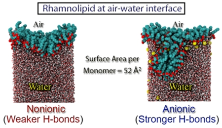
Our group has studied the aggregation properties of the most common monorhamnolipid congener, α-rhamnopyranosyl-β-hydroxydecanoyl-β-hydroxydecanoate ((R,R)-Rha–C10-C10), under conditions in which it exists in the nonionic and anionic form using molecular dynamics (MD) simulations.^10,11 Several interesting results were reported on the structure and stability of the aggregates in bulk water. The most important observation is that anionic Rha–C10-C10 prefers to form micellar aggregates in addition to large lamellar vesicles, and nonionic Rha–C10-C10 prefers lamellar vesicles over small micellar aggregates. It was shown that the hydrogen bonding interaction between the monomers in the aggregates is largely responsible for the observation of micellar aggregates in anionic Rha–C10-C10. The lack of the hydrogen bonding interaction between the monomers in small micellar aggregates directs the formation of larger lamellar vesicles where the stability is achieved in the form of a strong hydrophobic interaction due to the bilayer arrangement of the alkyl chains. It should be noted that these findings are fully complemented by the experimental observations.¹⁰

It is well-known that the aggregation of surfactants at the interface is crucial to many technological applications.^12,13 The critical micelle concentration (CMC) is an important characteristic of a surfactant, and aggregation of a surfactant at the interface is vital in determining the CMC of a surfactant. The interface must be fully saturated before the surfactant can enter the bulk water to form micellar aggregates. Recent experimental observations have shown that the aggregation properties of nonionic and anionic Rha–C10-C10 at the air–water interface are completely different.¹⁴ The surface area per surfactant at the CMC is ~117 ± 12 Ų for the anionic (R,R)-Rha–C10-C10, and it is ~21 ± 4 Ų for the nonionic form. It should be mentioned that the surface area per surfactant for native anionic monorhamnolipid mixtures available from the literature are 66 (pH 7),¹⁵ 77 (pH 9),¹⁵ and 86 Ų (pH 8).¹⁰ Our earlier publications describing the difference in behavior of nonionic and anionic Rha–C10-C10 aggregates in bulk water motivated us to study the observed difference in aggregation at the air–water interface.¹¹ In the present study, we have addressed the aggregation of anionic and nonionic Rha–C10-C10 at the air–water interface with major focus on the structure and stability of aggregation. Further calculations were also performed to understand the aggregation of Rha–C10-C10 at the oil–water interface. Additional simulations were carried out to study the structural properties of a bilayer in bulk water.

SIMULATION METHODS

Simulation of Rha–C10-C10 at the Air–Water and Oil–Water Interfaces.

MD simulations were employed to gain insight into the structural properties of Rha–C10-C10 molecules at the air–water interface and oil–water interface. In the present article, we have studied systems composed of 25–70 molecules of the most common congener in the native Rha–C10-C10 mixture in its nonionic and anionic forms (Scheme 1). Details of the force field parameters for the Rha–C10-C10 are available in our earlier publications.^10,11 Parameters for Rha–C10-C10 were obtained from the CHARMM (chemistry at Harvard macromolecular mechanics) General Force Field (version 2b8)¹⁶ and optimized according to the CHARMM force field¹⁷ parametrization procedure to better reproduce the properties of Rha–C10-C10 at a high level of ab initio calculation. Comparing the available experimental results validated the force field parameters obtained in this method. It is evident from our earlier work that anionic Rha–C10-C10 in bulk water forms micelles where the most probable aggregation number is ~36, which matches well with our calculations of ~40. The radii of the aggregates are also comparable to the experimental results.

Scheme 1.

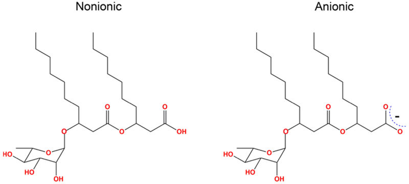
Molecular Structure of Nonionic and Anionic Monorhamnolipid

An initial starting structure for the air–water/oil–water interface was needed. The initial coordinates of the simulation were obtained with the help of PACKMOL software.¹⁸ A monolayer of the surfactant was prepared by randomly placing Rha–C10-C10 molecules inside a box such that one end of the box hosted the hydrophilic part, while the other end had hydrophobic alkyl chains. It should be noted that the anionic Rha–C10-C10 monolayer was neutralized with the addition of an equal number of sodium counterions (Na⁺ ). The x- and y-dimensions of the box are provided in the Table 1, and the z-axis of the box is close to the size of Rha–C10-C10, as shown in Scheme 2a.

Table 1.

Composition and Dimensions of the Simulated System for Rha–C10-C10 Surfactants at the Air–Water Interface

no. of Rha–C10-C10 (N)	no. of water molecules (nonionic)	no. of water molecules (anionic)	no. of Na+ ions (anionic)	initial box size (Å × Å × Å)	vacuum above monolayer (Å)	SAPM (Å2)	simulation time (ns)
25	17084	17075	25	60 × 60 × 340	90	144.0	37
30	17079	17072	30	60 × 60 × 340	90	120.0	37
35	17081	17069	35	60 × 60 × 340	90	102.9	37
40	17074	17071	40	60 × 60 × 340	90	90.0	37
45	17080	17062	45	60 × 60 × 340	90	80.0	37
50	17070	17045	50	60 × 60 × 340	90	72.0	37
55	17074	17059	55	60 × 60 × 340	90	65.5	37
60	17076	17049	60	60 × 60 × 340	90	60.0	37
65	17064	17041	65	60 × 60 × 340	90	55.4	37
70	17034	17025	70	60 × 60 × 340	90	51.4	37

Scheme 2.

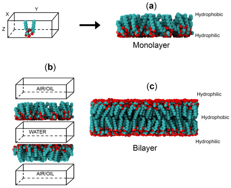
Representation of Monolayer, Air–Water Interface, Oil–Water Interface, and Bilayer Systems Used in the Study

For air–water/oil–water interface calculations, two monolayers were created and were placed above and below a pre-equilibrated TIP3P water box. The hydrophobic ends of the monolayers were filled with decane for the oil–water interface, and it was empty for the air–water interface, as shown in Scheme 2b. It should be noted that the x- and y-dimensions of the monolayer, water box, and vacuum/oil were all equal. The length of the z-axis of the water box separating the two surfactant monolayers was chosen as 150 Å in the present study. Starting structures for the bilayer simulations were prepared by placing one monolayer on top of the other, such that the hydrophobic ends face each other, as shown in Scheme 2c. The prepared bilayer structure was then solvated with water molecules for further simulations.

Starting with the initial configuration prepared, MD simulations were conducted with periodic boundary conditions using NAMD 2.9.¹⁹ A direct cutoff for nonbonded interactions of 1 nm, a switch function starting at 0.8 nm for cutoff of van der Waals interactions, and particle mesh Ewald²⁰ for long-range electrostatics were applied. The SHAKE algorithm²¹ was used to constrain all bonds involving hydrogen atoms, and a time step of 1 fs was used for the MD integration. The temperature and pressure were controlled, respectively, by the Langevin thermostat and the Nose–Hoover Langevin barostat,^22,23 as implemented in NAMD. The system was first energy minimized, then heated to 300 K, and finally equilibrated under constant 1 atm pressure and temperature. It should be mentioned that the constant pressure was applied in a direction perpendicular to the interface. During minimization, heating, and equilibration, no constraints were applied. A production run was performed on the fully equilibrated system to analyze the structural properties of the Rha–C10-C10 molecules at the air–water interface. Figure 1 shows the initial structure and the equilibrated structure after 37 ns of simulation for nonionic Rha–C10-C10 at the air–water interface.

Figure 1.

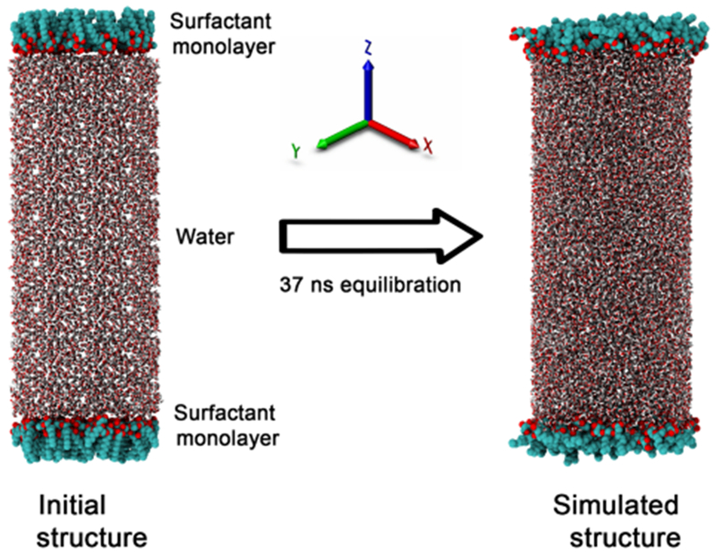
Initial and simulated air–water interface system used in the study. The two monolayers are separated by a water box.

RESULTS AND DISCUSSION

In the present study, two different sets of system were considered for simulation to better understand the aggregation of Rha–C10-C10 at the air–water interface. The first set is composed of systems where the surface area of the box (XY) is kept constant, and the number of monomers at the interface is varied from 25 to 70. Table 1 presents the details of the first set of systems. The second set is composed of various systems where the XY dimensions of the simulation box are varied, while keeping the number of monomers a constant 50 at the interface. Table 2 presents the details of the second set of systems considered for the study. The aim of having two sets of systems is to have a clear understanding of the aggregation of nonionic and anionic Rha–C10-C10 at the air–water interface.

Table 2.

Composition and Dimensions of the Simulated System for MD Simulations of Rha–C10-C10 Surfactants at the Air–Water Interface

no. of Rha–C10-C10 (N)	no. of water molecules (nonionic)	no. of water molecules (anionic)	no. of Na+ ions (anionic)	initial box size (Å × Å × Å)	vacuum above monolayer (Å)	SAPM (Å2)	simulation time (ns)
50	12845	12837	50	52 × 52 × 340	90	54.1	37
50	13869	13843	50	54 × 54 × 340	90	58.3	37
50	14913	14888	50	56 × 56 × 340	90	62.7	37
50	16071	16044	50	58 × 58 × 340	90	67.3	37
50	17070	17045	50	60 × 60 × 340	90	72.0	37
50	18380	18349	50	62 × 62 × 340	90	76.9	37
50	19681	19655	50	64 × 64 × 340	90	81.9	37
50	20843	20829	50	66 × 66 × 340	90	87.1	37
50	22099	22075	50	68 × 68 × 340	90	92.5	37
50	24719	24700	50	72 × 72 × 340	90	103.7	37
50	27600	27583	50	76 × 76 × 340	90	115.5	37
50	30688	30670	50	80 × 80 × 340	90	128.0	37
50	33899	33874	50	84 × 84 × 340	90	141.1	37

Monolayer Separation Distance.

Figure 1 presents a representative initial and simulated air–water interface system used in this study. The simulation of the surfactant at the air–water interface is carried out by placing two monolayers separated by a water box. It is important that the monolayers are sufficiently far from each other and the water box separating them should be long enough (z-axis). The length of the z-axis was tested by MD simulations with lengths ranging from 80 to 160 Å, with an increment of 10 Å. The interface formation energy (IFE) of Rha–C10-C10 in the simulated systems were calculated to find out the effect of various intermonolayer distances. The IFE is a measure of the average intermolecular interactions per surfactant molecule arising from the insertion of one surfactant molecule into the air–water interface.

One of methods available in the literature to evaluate the IFE is defined below.^24,25

$$\mathrm{IFE}=(E_{\text{total}}-(n\times E_{\text{surfactant,single}}+E_{\text{air-water}}\left)\right)∕n$$

where E_total denotes the energy of the whole system, E_{surfactant,single} denotes the energy of a single surfactant molecule calculated from a separate MD simulation in a vacuum at the same temperature, and E_air–water denotes the bare air–water system obtained from a separate MD simulation of the water box with the same number of water molecules used in the total system at the same temperature.

The results of IFE as a function of the water box length along the z-axis are presented in Figure 2. The figure shows that the IFE values oscillate within a 2 kcal/mol range. In the present study, we choose 150 Å as the z-axis length of the water box separating the monolayers. It is shown later in the discussion that the density of water equidistant from the monolayers compares well with the density of the bulk water. Therefore, all of the air–water and oil–water interface simulations in the present study are carried out using a water box with a z-axis length of 150 Å.

Figure 2.

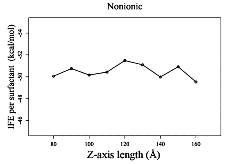
IFE of Rha–C10-C10 as a function of the z-axis length of the water box separating the two monolayers.

Surface Concentration.

The most probable surface concentration is an important quantity that provides information about the surface area occupied by a surfactant at the interface when in equilibrium. One of methods available in the literature to predict the most probable surface concentration is to evaluate the IFE. Figure 3 presents the IFE as a function of surface area occupied by a surfactant for nonionic and anionic Rha–C10-C10 obtained from air–water MD simulations. It is evident from the figure that the most probable surface concentration occurs when the surface area per molecule (SAPM) is at 80 Ų in both the nonionic and anionic forms. It is surprising to see that there is no difference in SAPM at the most likely surface concentration, despite the fact that one of them is charged and other is neutral.

Figure 3.

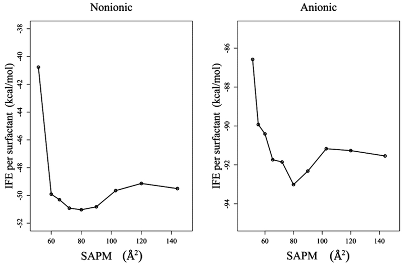
IFE as a function of surface area occupied by each monomer at the air–water interface.

Surface Pressure–Area Isotherm.

The predicted surface pressure–area isotherms for nonionic and anionic Rha–C10-C10 are depicted in Figure 4. The procedure to obtain surface pressure can be found elsewhere and references therein.^24,26 The surface pressure of a monolayer is a more convenient quantity for direct comparison between simulations and experimental data. First, it is clearly observed that the surface pressure decreases with increasing area/molecule. At low surface concentration, the monolayer is in a gas-like phase, and the surface pressure approaches zero. As we increase the concentration of the surfactant, the molecules begin to interact with each other due to the decreasing area per monomer. At a certain surface concentration, the surface pressure increases as the monolayer becomes more populated. The results also indicate that anionic and nonionic Rha–C10-C10 at the air–water interface have a similar pressure–area isotherm. It should be mentioned that the experiments performed on Rha–C18-C18 at the air–water interface show similar behaviors.²⁷ Similar to the IFE analysis, the present pressure–area isotherm does not provide any distinguishing information to understand the observed experimental differences seen in nonionic and anionic Rha–C10-C10 aggregation at the air–water interface.

Figure 4.

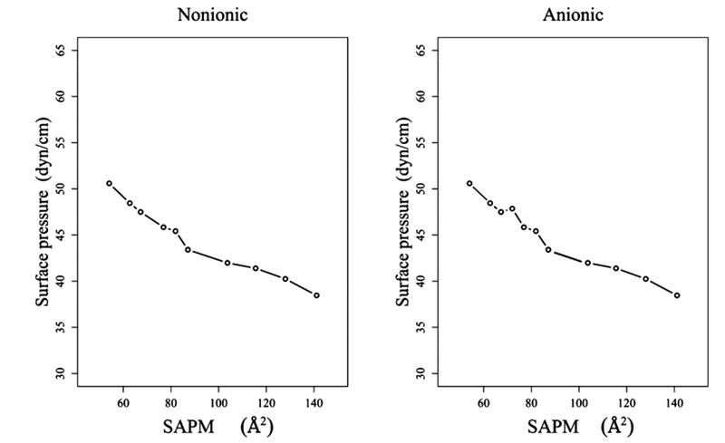
Pressure–area isotherms for the air–water interface systems.

Structure of the Monolayers.

We analyzed the structure of monolayer to detect any difference between the anionic and nonionic Rha–C10-C10. Representative snapshots of the configurations for nonionic and anionic Rha–C10-C10 monolayers at various surface concentrations are given in Figure 5. At low surface concentrations, the Rha–C10-C10 are dispersed across the interface, and the alkyl chains are randomly oriented. There is little aggregation and no obvious formation of surfactant domains at the interface. As the surface coverage is increased, the surfactant alkyl chains interact with each other and are vertically oriented to some extent. At complete surface coverage SAPM = 80 Ų, the monolayer is nearly flat, and the surfactant molecules are evenly distributed at the interface. It is possible to see the hydrophobic tails interacting more and hydrophilic headgroups interacting with water molecules. It should be noted that there is no structural difference in the monolayer aggregation between anionic and nonionic Rha–C10-C10 at complete surface coverage concentration.

Figure 5.

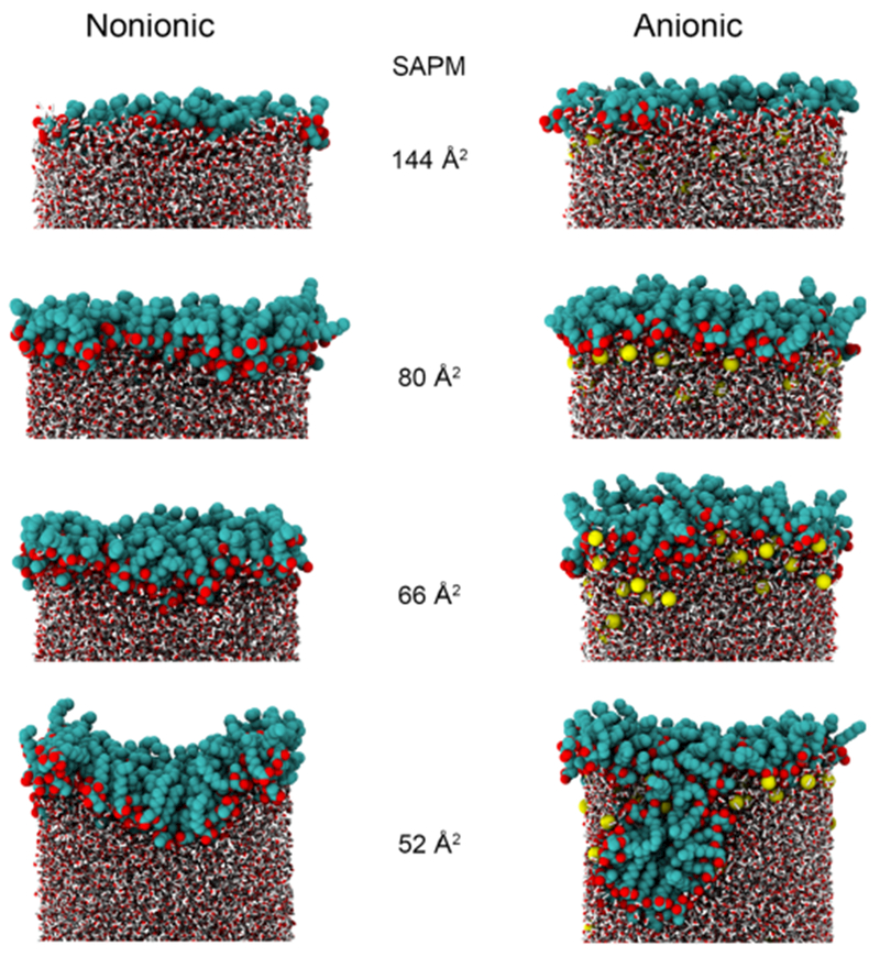
Snapshots of the anionic and nonionic monolayers at different surface coverages. Rha–C10-C10 are shown as VDW spheres, and water molecules are shown as smaller tubes. For anionic monolayers, the sodium counterions are shown as yellow spheres.

As the surface coverage is increased further, the monolayers start to exhibit undulations. The extent of monolayer undulations is greater in anionic than nonionic Rha–C10-C10. It is interesting to see that at SAPM = 52 Ų, the monolayer undulation is leading to a near formation of the micellar aggregate for anionic Rha–C10-C10. Therefore, it is evident from the structure of monolayers that anionic and nonionic Rha–C10-C10 aggregation is similar at the complete surface coverage concentration, but they differ at higher surface concentrations. Insights into those properties are provided below.

Density Profiles of Monolayers at Complete Surface Coverage Concentration.

To gain further insight into different aggregation properties of nonionic and anionic Rha–C10-C10 at the air–water interface, we analyzed the density profiles of the surfactant monolayers over the last 5 ns of the simulations. Mass density analysis of the anionic and nonionic Rha–C10-C10 monolayers were obtained using VMD, as described in the literature.²⁸ Figure 6 shows the mass density profiles of the air–water interface system along the z-axis direction of the simulation box. It should be mentioned that the density of bulk water, 0.6 g/mol/ų (997 kg/m³), is in good agreement with the experimental water density, 998 kg/m³. This indicates that our systems are, indeed, large enough to allow the water to reach its bulk properties, and the two resulting interfaces are independent and do not interfere with each other. Figure 6a,b shows little difference between the monolayers of nonionic and anionic monolayers.

Figure 6.

Mass density profiles of (a) nonionic and (b) anionic Rha–C10-C10 air–water interface systems. A closer look into the mass density of (c) nonionic and (d) anionic Rha–C10-C10 monolayers.

A closer look at the monolayer is provided in Figure 6c,d. Once again, we see that there is no significant difference in the position of the mass densities of most of the groups of Rha–C10-C10. The notable differences are found in the distribution of the carboxylic group and rhamnose group of the Rha–C10-C10 in the monolayer. The rhamnose group appears to be slightly better hydrated in the nonionic monolayer than in the anionic. This could be due to the availability of the carboxylic group to form hydrogen bonds with the rhamnose group in nonionic Rha–C10-C10. This hydrogen bonding interaction makes the rhamnose groups place themselves closer to the carboxylic group and be more strongly hydrated. The carboxylic group density distribution is wider in nonionic, whereas it is moderately sharp in the anionic monolayer. In the case of anionic monolayer, the concentration of sodium counterions (Na⁺) near the interface attracts the more carboxylic group toward it due to the strong Na⁺ ···O⁻ interaction. The counterions also attract more water molecules, causing the density of the water to increase slightly near the interface. Therefore, the mass density of the monolayers of the nonionic and anionic Rha–C10-C10 shows differences in the position of the carboxylic group and rhamnose group. It is likely that the headgroup conformations of the Rha–C10-C10 at the interface could be a reason for the different mass density profiles.

Headgroup Conformation.

It is well-known that Rha–C10-C10 is structurally different from conventional surfactants. Conventional surfactants have a polar headgroup well separated from the nonpolar tail group. The situation is entirely different in Rha–C10-C10, as there are no well-defined regions for hydrophilic and hydrophobic groups. Hydrophilic regions, such as the carboxylic group, the rhamnose group, and an ester linkage, are spread across the molecule with two alkyl chains positioned in between them. It is worth analyzing the conformation of these molecules at the air–water interface to understand their aggregation properties. It should be noted that the density profiles of monolayers at the complete surface coverage concentration showed that the position of carboxylic groups and rhamnose groups are different in nonionic and anionic Rha–C10-C10. In this study, we have used the same method that was employed in our previous work to analyze the headgroup conformations of Rha–C10-C10 at the air–water interface.¹¹

Figure 7 presents the headgroup conformations of Rha–C10-C10 at the air–water interface for complete surface coverage concentrations (left) and higher concentrations (right). The x-axis is the intramolecular distance measured between the carboxylic group and the rhamnose group (which we refer to as the “headgroup conformation”). The distances are measured for all of the monomers present in the system along the trajectory consisting of 500 frames. Each count on the y-axis refers to the number of monomers in the corresponding headgroup conformation. It is seen from the plots that there are four major conformations (1, 2, 3, and 4) of Rha–C10-C10 molecules at the interface. The small peak at ~11 Å is observed for both anionic and nonionic Rha–C10-C10. It is to be noted, that the position and size of the peaks are identical and correspond to a fully open conformation (2).

Figure 7.

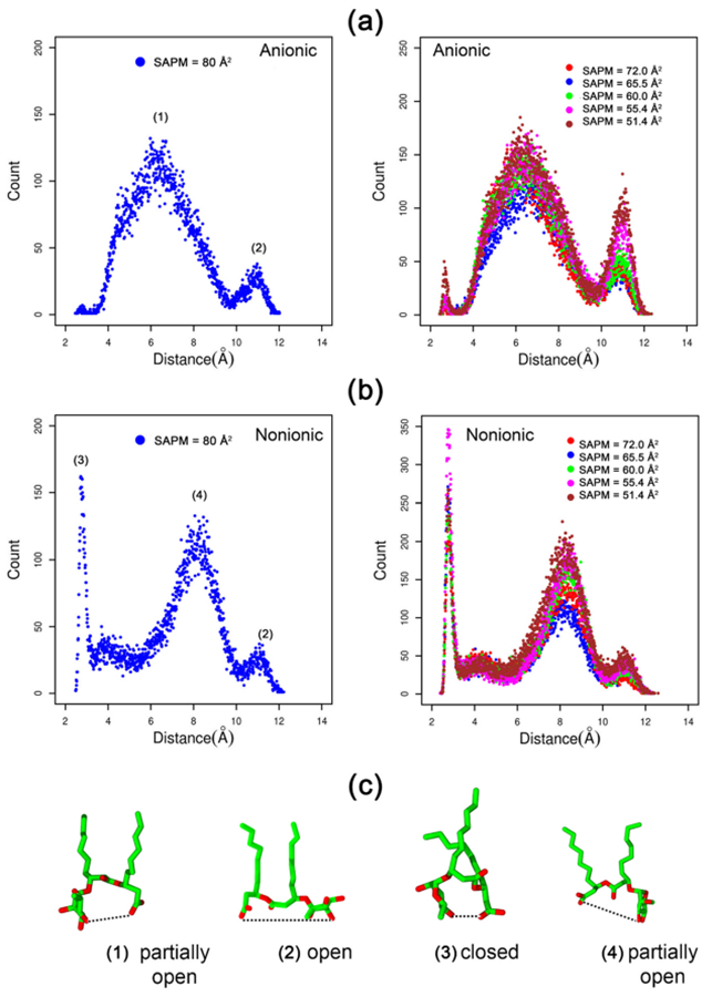
Headgroup conformation of the Rha–C10-C10 monomers in the monolayers (a) anionic and (b) nonionic at the air–water interface. Corresponding structures of monomers are also provided.

The major difference between the nonionic and anionic Rha–C10-C10 monolayers is evident from the peaks 1, 3, and 4. The headgroup conformations of anionic Rha–C10-C10 at the air–water interface predominantly peak near ~6.0 Å. This peak corresponds to a partially open conformation (1). On the other hand, nonionic Rha–C10-C10 at the air–water interface has two competing headgroup conformations, as seen from the peaks near ~3.0 and ~9.0 Å. The peak near ~3.0 Å corresponds to a fully closed conformation (3), whereas the peak at ~9.0 Å corresponds to a half open conformation (4). It is interesting to see that anionic Rha–C10-C10 at the interface has the least preference for a fully closed headgroup conformation. The cause for this could be the less desirable hydrophobic interactions of the alkyl chains and not an effective packing of the chains. It is also evident from the plots that the headgroup conformational preferences of nonionic and anionic Rha–C10-C10 at the air–water interface do not change with increasing concentration. It is very important to note, that the headgroup conformations at the complete surface coverage concentration and higher concentrations are similar. It is therefore clear from the above analysis that the headgroup conformations of nonionic and anionic Rha–C10-C10s are completely different at the air–water interface. This could be one of the driving forces for the differences observed in Figure 5. The preferred headgroup conformation of anionic Rha–C10-C10 is just the right orientation for possible hydrogen bonding interactions between the monomers, as will be revealed in the h-bond analysis below.

H-Bonding Interaction in Monolayers.

The significant difference between the headgroup conformations of anionic and nonionic Rha–C10-C10 at the air–water interface prompted us to analyze the hydrogen bonding interaction between the monomers. Hydrogen bonding interactions between the monomers at the interface were calculated at each frame along a 5 ns trajectory for both nonionic and anionic Rha–C10-C10 monolayers. Hydrogen bonds were identified using the cutoff conditions that H-bond distances between electronegative atoms are ≤3.0 Å, and H-bond O–O–H angles are ≤20°. The occupancy of a hydrogen bond is 100% if it exists in all of the frames along the trajectory. The calculated hydrogen bond occupancy is presented in Figure 8 for the anionic and nonionic Rha–C10-C10 monolayers at (a) complete surface coverage concentration and (b) at higher concentrations. It is clearly evident from the figure, that the occupancy of hydrogen bonding interaction in nonionic is less than 50%, with most of them around 0% occupancy. Hydrogen bonds in the nonionic monolayer are forming and breaking constantly. The nonionic monolayer encounters a larger number of hydrogen bonds, but most of them are weak and less stable. On the other hand, the hydrogen bond occupancy of the anionic monolayer is higher compared to that of nonionic monolayer, many of them >50%. In a few cases, the occupancy is more than 100%, indicating that existence of multiple hydrogen bonds involving a single atom. A representative example provided in the figure shows that carboxylic oxygen forms a bifurcated hydrogen bonding with two of the hydroxyl groups of the rhamnose ring. This shows that the hydrogen bonding interactions in the anionic monolayer are stronger and more stable with some of them seen throughout the trajectory.

Figure 8.

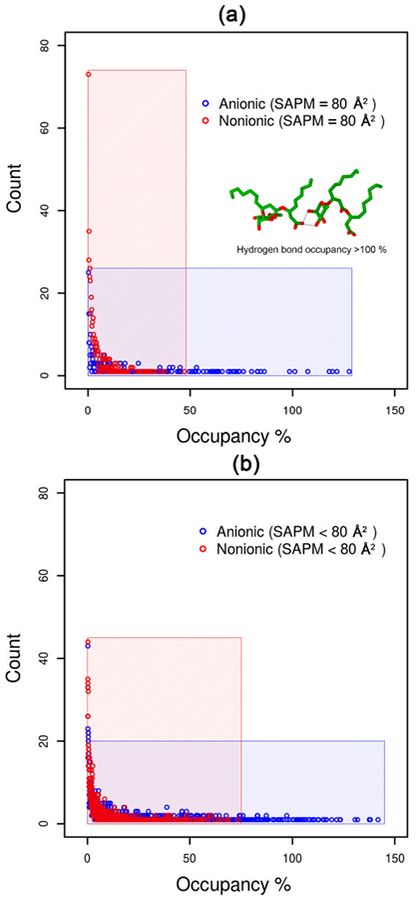
Hydrogen bond occupancy at complete surface coverage concentration and higher concentration of Rha–C10-C10 at the air–water interface.

The differences observed between the anionic and nonionic monolayer based on the headgroup conformation and hydrogen bond occupancy helps explain the snapshots shown in Figure 5. Strong and more stable hydrogen bonding interactions between the monomers in the anionic monolayer cause the segregation of small aggregates from the monolayer, which then forms micelles. Weak and less stable hydrogen bonding interactions between the monomers in the nonionic monolayer do not help the segregation of smaller aggregates from the monolayer. As a consequence, anionic Rha–C10-C10 form micelles with a lower concentration of surfactants compared to that of nonionic Rha–C10-C10 at the air–water interface.

The critical micelle concentration is the concentration at which micelles appear in the solution. In the case of anionic Rha–C10-C10, the micelles are observed in bulk water faster than nonionic Rha–C10-C10. In other words, the concentration of anionic Rha–C10-C10 needed to form micelle in bulk water is less than the concentration of nonionic Rha–C10-C10 required. If the surface area and concentration of the surfactants at CMC are known, we could address this observation in terms of SAPM. The experiments have shown that SAPM at the CMC for anionic Rha–C10-C10 is ~100 Ų, whereas for nonionic Rha–C10-C10, the SAPM is ~25 Ų. Our simulation studies have shown that the conformations of anionic Rha–C10-C10 are completely different than those of nonionic Rha–C10-C10. This conformational difference enhances the hydrogen bonding interaction between the monomers in the anionic Rha–C10-C10 monolayer but does not support hydrogen bonds in the nonionic Rha–C10-C10 monolayer. The presence of persistent hydrogen bonds enables the formation of micelles in anionic compared to nonionic. Therefore, the structural properties of the molecular aggregation at the air–water interface discussed in the present investigation explain the differential aggregation properties of nonionic and anionic Rha–C10-C10 at the air–water interface.

Structural Properties of the Bilayers.

It is well-known, that the lipid bilayers are the universal basis for cell membrane structure. These bilayer structures are attributable to the special properties of the amphiphilic molecules, which cause them to assemble spontaneously into bilayers in aqueous environment. In the present study, we analyze the bilayer structure of Rha–C10-C10 to complement the properties observed for monolayer aggregation at the air–water interface. We focus more on the headgroup conformation and hydrogen bond occupancy for the reason that these two properties are the basis for the difference in the aggregation phenomenon at the air–water interface. One cannot expect identical properties for the monolayer at the interface and bilayer in bulk water, but they should have similar properties because their aggregation is spontaneous. Figure 9 presents the representative snapshots of the bilayer structure of nonionic and anionic Rha–C10-C10 in bulk water. The XY dimensions of the simulation box is 100 Ų in both cases. The number of Rha–C10-C10 in each monolayer is 160, and that makes a total of 320 molecules in the bilayer. It is possible to note from the figure that the bilayers show undulations, and it could be due to the short alkyl chains and uneven distribution of the headgroups.

Figure 9.

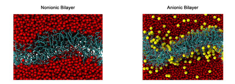
Representative snapshots of bilayers of nonionic and anionic Rha–C10-C10. Water molecules are shown as red spheres, and sodium counterions are shown as yellow spheres. Hydrogen atoms are removed for clarity.

The headgroup conformations and hydrogen bond occupancy of the bilayers are calculated and presented in Figure 10. As we can see from the figure, the structural properties of the monolayer at the air–water interface is very much similar to the bilayer structure in bulk water. Nonionic Rha–C10-C10 prefers two major headgroup conformations, while the anionic Rha–C10-C10 prefers a single conformation. The hydrogen bonding occupancy is less than 50% for nonionic Rha–C10-C10, and it is more than 50% and even higher than 100 in some cases. These observations complement the results obtained for the monolayer aggregation at the air–water interface.

Figure 10.

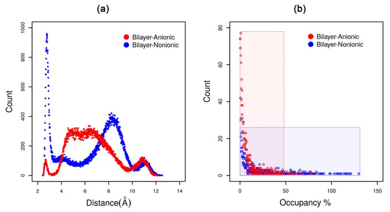
Structural properties of the Rha–C10-C10 bilayer (a) headgroup conformations and (b) hydrogen bond occupancy.

Oil–Water Interface Properties.

Rhamnolipids are an excellent candidate for the enhanced oil recovery process. In the present study, we try to understand the interfacial properties and monolayer stability of Rha–C10-C10 at the oil–water interface. It was shown in the previous section, that nonionic and anionic Rha–C10-C10 show differential structural properties, which in turn leads to a completely different SAPM at the CMC. The stability of the monolayers at the air–water interface is significantly governed by the headgroup conformation and hydrogen bonding interactions of the monomers, in addition to various other factors. Hydrophobic interactions arising from the alkyl chains of Rha–C10-C10 have little contribution to the aggregation properties. The situation is different when it comes to the oil–water interface. The alkyl chains are now in contact with the oil surface, and it should be interesting to see how it exploits the hydrophobic interaction for the aggregation behavior of nonionic and anionic Rha–C10-C10 at the oil–water interface.

In the present study, we have performed MD simulations of nonionic and anionic Rha–C10-C10 at an oil–water interface. Decane molecules were used as the representative oil molecules in the simulation. Table 3 presents the complete list of systems used for the oil–water interface simulations. The simulations were carried out for systems where the SAPM at the oil–water interface is ≤87 Ų. We characterized the interfacial structure by calculating the monolayer thickness, density profiles, headgroup conformations, and hydrogen bonding interactions.

Table 3.

System Information for Oil–Water Interface Simulations^a

no. of Rha–C10-C10 (N)	no. of decane molecules (nonionic)	no. of decane molecules (anionic)	no. of Na+ ions (anionic)	initial box size (Å × Å × Å)	SAPM (Å2)	simulation time (ns)
50	445	445	50	50 × 50 × 290	50.0	35
50	485	485	50	52 × 52 × 290	54.1	35
50	525	525	50	54 × 54 × 290	58.3	35
50	565	565	50	56 × 56 × 290	62.7	35
50	605	605	50	58 × 58 × 290	67.3	35
50	645	645	50	60 × 60 × 290	72.0	35
50	690	690	50	62 × 62 × 290	76.9	35
50	735	735	50	64 × 64 × 290	81.9	35
50	780	780	50	66 × 66 × 290	87.1	35

^aThe number of surfactants and oils provided in the table corresponds to a single monolayer.

Monolayer Thickness.

To gain insights into the monolayer structures, we analyzed the density profiles of the surfactant monolayers over the last 10 ns of the simulations. Representative snapshots of the oil–water interface systems for three different surface concentrations are shown in Figure 11. The interfacial thickness of a complex interface, such as the decane–water interface in the presence of surfactants, is not easily defined. We have used the procedure adopted in the literature to define the monolayer thickness.²⁹ The thickness is defined as the distance between the two positions where the densities of the decane and water phases are at 90% of their respective bulk densities. Figure 12 presents the measured interfacial thickness of the nonionic and anionic monolayer at the oil–water interface for various surface concentrations. The interfacial thickness value increases with increasing SAPM for both forms of Rha–C10-C10. This is because the presence of the hydrophobic decane phase makes the alkyl chains of Rha–C10-C10 more vertically oriented, thus increasing the interfacial thickness. We can see from the figure that the monolayer thickness is similar for nonionic and anionic Rha–C10-C10 near complete surface coverage concentrations, SAPM ~ 80 Ų. But at higher surface concentrations, the anionic monolayer is about ~10 Å thicker than that of the nonionic monolayer. This indicates that the diffusion of the anionic Rha–C10-C10 into the bulk phases is increased compared to those of the nonionic Rha–C10-C10. The hydrophobic interactions between the alkyl chains and decane phase have no significant effect on the aggregation of nonionic and anionic Rha–C10-C10 at the oil–water interface compared to that at the air–water interface. The representative snapshots shown in Figure 11 support the observation, and these figures are similar to the air–water interface figures.

Figure 11.

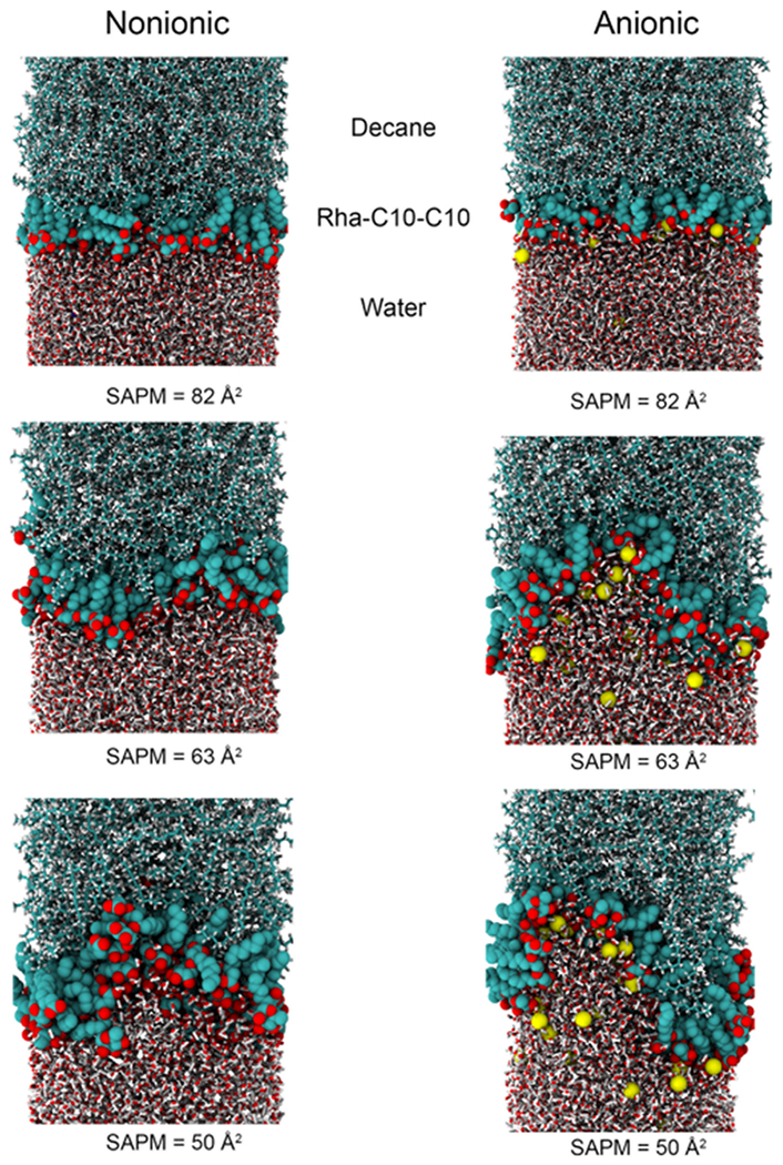
Representative snapshots of the Rha–C10-C10 monolayer at the oil–water interface for three different surface concentration.

Figure 12.

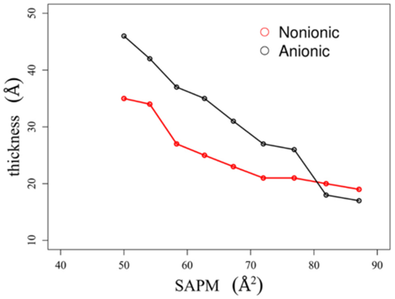
Thickness of the nonionic and anionic monolayers at the oil–water interface as a function of SAPM.

Mass Density Profiles.

To gain insights into the monolayer structures, we analyzed the density profiles of the surfactant monolayers over the last 10 ns of the simulations. The profiles of the monolayer corresponding to SAPM = 82 Ų is provided in Figure 13. The figure shows that the densities of decane and water phases approach the bulk densities of decane and water, respectively. Therefore, the two resulting interfaces are independent of each other. The density profiles of nonionic and anionic monolayers look similar. The notable difference is the distribution of the rhamnose ring, which is much wider in the anionic monolayer. This could be due to the hydrophobic interactions between alkyl chains and decane molecules pulling the rhamnose ring in one direction, and the ionic interactions between the carboxylic group and sodium ions pulling the rhamnose ring in the opposite direction. This could probably be a consequence of the strong desire of the methyl group at the sixth position on the rhamnose ring to want to be near the decane molecules. It should be noted that rhamnose is one of the most hydrophobic sugars. These two interactions make the density profile of the rhamnose ring much wider compared to the nonionic monolayer. Density profiles of other components look similar to the air–water interface density profiles. The carboxylic headgroup of all of the Rha–C10-C10 are always found entirely within the water phase similar to the air–water profile.

Figure 13.

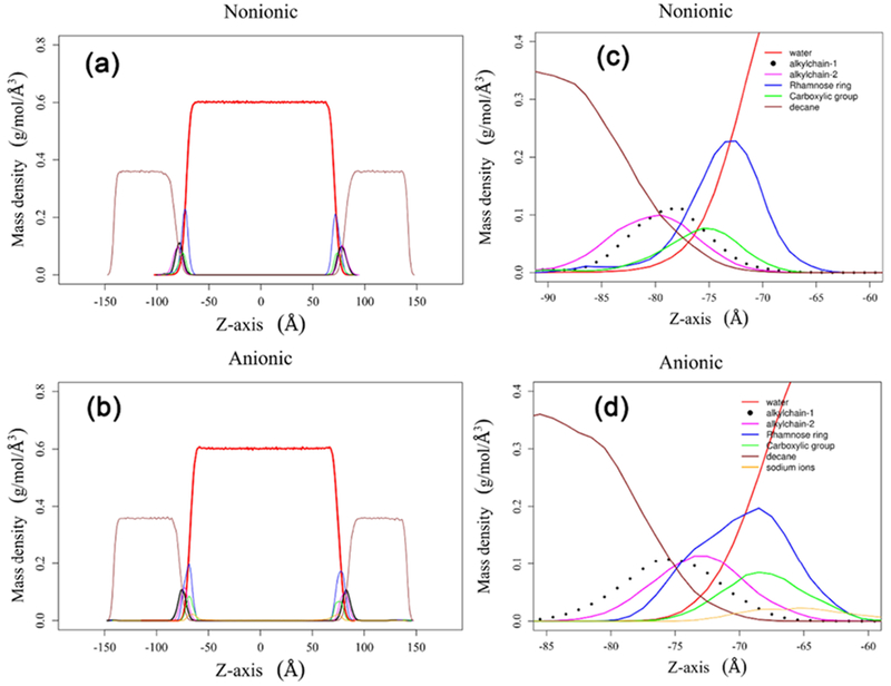
Mass density profiles of (a) nonionic and (b) anionic Rha–C10-C10 oil–water interface systems. (b) A closer look into the mass density of (c) nonionic and (d) anionic Rha–C10-C10 monolayers.

Headgroup Conformation and Hydrogen Bond Occupancy.

The headgroup conformations and hydrogen bond occupancy of the monolayers are presented in Figure 14. As we can see from the figure, the structural properties of the monolayer at the oil–water interface are very much similar to the air–water interface and bilayer structure in bulk water. Nonionic Rha–C10-C10 prefers two major headgroup conformations, while the anionic Rha–C10-C10 prefers a single conformation. The hydrogen bonding occupancy is less than 50% for nonionic Rha–C10-C10, and it is more than 50% and even higher than 100% in some cases. These observations show that the structural properties of nonionic and anionic Rha–C10-C10 are not affected by the different interfaces or bulk water.

Figure 14.

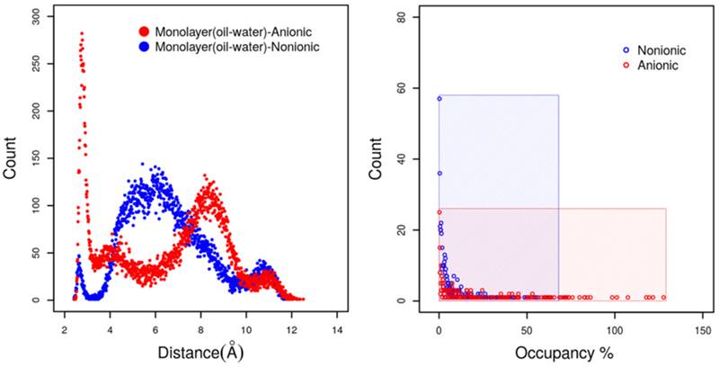
Headgroup conformations and hydrogen bond occupancy of nonionic and anionic Rha–C10-C10 at the oil–water interface.

CONCLUSIONS

Understanding the effect of the surfactant structure on interfacial properties is of great scientific and industrial interest. Rhamnolipids are important biosurfactants on which extensive experimental research work has been carried out, and it is equally important that theoretical studies be carried out to complement the results and provide vital structural information. In this study, we have investigated the aggregation properties of anionic and nonionic Rha–C10-C10 at the air–water and oil–water interfaces. We have characterized the interfacial structures and their properties in details using MD simulations to elucidate the differential aggregation behavior observed in experiment. These calculations rationalize the drastically different experimental values for SAPM for nonionic and anionic rhamnolipids and suggest that simple, complete surface coverage calculations do not always yield all explanations of experimental results.

REFERENCES

- (1).Van Bogaert IN; Saerens K; De Muynck C; Develter D; Soetaert W; Vandamme EJ Microbial production and application of sophorolipids. Appl. Microbiol. Biotechnol 2007, 76, 23–34. [DOI] [PubMed] [Google Scholar]
- (2).Mann RM; Boddy MR Biodegradation of a nonylphenol ethoxylate by the autochthonous microflora in lake water with observations on the influence of light. Chemosphere 2000, 41, 1361–1369. [DOI] [PubMed] [Google Scholar]
- (3).Mann RM; Bidwell JR The acute toxicity of agricultural surfactants to the tadpoles of four Australian and two exotic frogs. Environ. Pollut 2001, 114, 195–205. [DOI] [PubMed] [Google Scholar]
- (4).Dobler L; Vilela LF; Almeida RV; Neves BC Rhamnolipids in perspective: gene regulatory pathways, metabolic engineering, production and technological forecasting. New Biotechnol. 2016, 33, 123–135. [DOI] [PubMed] [Google Scholar]
- (5).Burger MM; Glaser L; Burton RM The Enzymatic synthesis of a rhamnose-containing glycolipid by extracts of pseudomonas aeruginosa. J. Biol. Chem 1963, 238, 2595–2602. [PubMed] [Google Scholar]
- (6).Abdel-Mawgoud AM; Lepine F; Deziel E Rhamnolipids: Diversity of structures, microbial origins and roles. Appl. Microbiol. Biotechnol 2010, 86, 1323–1336. [DOI] [PMC free article] [PubMed] [Google Scholar]
- (7).Jirku V; Cejkova A; Schreiberova O; Jezdik R; Masak J Multicomponent biosurfactants–A “Green Toolbox” extension. Biotechnol. Adv 2015, 33, 1272–1276. [DOI] [PubMed] [Google Scholar]
- (8).Lovaglio RB; Silva VL; Ferreira H; Hausmann R; Contiero J Rhamnolipids know-how: Looking for strategies for its industrial dissemination. Biotechnol. Adv 2015, 33, 1715–1726. [DOI] [PubMed] [Google Scholar]
- (9).Marchant R; Banat IM Biosurfactants: a sustainable replacement for chemical surfactants? Biotechnol. Lett 2012, 34, 1597–1605. [DOI] [PubMed] [Google Scholar]
- (10).Eismin R; Munusamy E; Kegel L; Hogan D; Maier R; Schwartz S; Pemberton J Evolution of aggregate structure in solutions of anionic monorhamnolipids: Experimental and computational Results. Langmuir 2017, 33, 7412–7424. [DOI] [PMC free article] [PubMed] [Google Scholar]
- (11).Munusamy E; Luft C; Pemberton J; Schwartz S Structural properties of nonionic monorhamnolipid aggregates in water studied by classical molecular dynamics simulations. J. Phys. Chem. B 2017, 121, 5781–5793. [DOI] [PMC free article] [PubMed] [Google Scholar]
- (12).Patist A; Jha BK; Oh SG; Shah DO Importance of micellar relaxation time on detergent properties. J. Surfactants Deterg 1999, 2, 317–324. [Google Scholar]
- (13).Patist A; Kanicky JR; Shukla PK; Shah DO Importance of micellar kinetics in relation to technological processes. J. Colloid Interface Sci 2002, 245, 1–15. [DOI] [PubMed] [Google Scholar]
- (14).Palos Pacheco R; Eismin RJ; Coss CS; Wang H; Maier RM; Polt R; Pemberton JE Synthesis and characterization of four diastereomers of monorhamnolipids. J. Am. Chem. Soc 2017, 139, 5125–5132. [DOI] [PubMed] [Google Scholar]
- (15).Chen ML; Penfold J; Thomas RK; Smyth TJP; Perfumo A; Marchant R; Banat IM; Stevenson P; Parry A; Tucker I; Grillo I Solution self-assembly and adsorption at the air–water interface of the monorhamnose and dirhamnose rhamnolipids and their mixtures. Langmuir 2010, 26, 18281–18292. [DOI] [PubMed] [Google Scholar]
- (16).Vanommeslaeghe K; Hatcher E; Acharya C; Kundu S; Zhong S; Shim J; Darian E; Guvench O; Lopes P; Vorobyov I; Mackerell AD Jr, CHARMM general force field: A force field for drug-like molecules compatible with the CHARMM all-atom additive biological force fields. J. Comput. Chem 2009, 31, 671–690. [DOI] [PMC free article] [PubMed] [Google Scholar]
- (17).Best RB; Zhu X; Shim J; Lopes PE; Mittal J; Feig M; Mackerell AD Jr, Optimization of the additive CHARMM all-atom protein force field targeting improved sampling of the backbone phi, psi and side-chain chi(1) and chi(2) dihedral angles. J. Chem. Theory Comput 2012, 8, 3257–3273. [DOI] [PMC free article] [PubMed] [Google Scholar]
- (18).Martinez L; Andrade R; Birgin EG; Martinez JM PACKMOL: A package for building initial configurations for molecular dynamics simulations. J. Comput. Chem 2009, 30, 2157–2164. [DOI] [PubMed] [Google Scholar]
- (19).Phillips JC; Braun R; Wang W; Gumbart J; Tajkhorshid E; Villa E; Chipot C; Skeel RD; Kale L; Schulten K Scalable molecular dynamics with NAMD. J. Comput. Chem 2005, 26, 1781–1802. [DOI] [PMC free article] [PubMed] [Google Scholar]
- (20).Darden T; York D; Pedersen L Particle mesh ewald - an N.Log(N) method for ewald sums in large systems. J. Chem. Phys 1993, 98, 10089–10092. [Google Scholar]
- (21).Ryckaert JP; Ciccotti G; Berendsen HJC Numerical-integration of cartesian equations of motion of a system with constraints - molecular-dynamics of n-Alkanes. J. Comput. Phys 1977, 23, 327–341. [Google Scholar]
- (22).Martyna G; Tobias D; Klein M Constant-pressure molecular-dynamics algorithms. J. Chem. Phys 1994, 101, 4177–4189. [Google Scholar]
- (23).Feller S; Zhang Y; Pastor R; Brooks B Constant-pressure molecular-dynamics simulation - the langevin piston method. J. Chem. Phys 1995, 103, 4613–4621. [Google Scholar]
- (24).Jang SS; Lin S-T; Maiti PK; Blanco M; Goddard WA; Shuler P; Tang Y Molecular dynamics study of a surfactant-mediated decane–water interface: Effect of molecular architecture of alkyl benzene sulfonate. J. Phys. Chem. B 2004, 108, 12130–12140. [Google Scholar]
- (25).Jang SS; Goddard WA Structures and properties of newton black films characterized using molecular dynamics simulations. J. Phys. Chem. B 2006, 110, 7992–8001. [DOI] [PubMed] [Google Scholar]
- (26).Gullingsrud J; Babakhani A; McCammon JA Computational investigation of pressure profiles in lipid bilayers with embedded proteins. Mol. Simul 2006, 32, 831–838. [Google Scholar]
- (27).Wang H; Coss CS; Mudalige A; Polt RL; Pemberton JE A PM-IRRAS investigation of monorhamnolipid orientation at the air–water interface. Langmuir 2013, 29, 4441–4450. [DOI] [PubMed] [Google Scholar]
- (28).Giorgino T Computing 1-D atomic densities in macromolecular simulations: The density profile tool for VMD. Comput. Phys. Commun 2014, 185, 317–322. [Google Scholar]
- (29).Tan JSJ; Zhang L; Lim FCH; Cheong DW Interfacial properties and monolayer collapse of alkyl benzenesulfonate surfactant monolayers at the decane–water interface from molecular dynamics simulations. Langmuir 2017, 33, 4461–4476. [DOI] [PubMed] [Google Scholar]
Associated Data
This section collects any data citations, data availability statements, or supplementary materials included in this article.