

Abstract
This paper proposes a method using multidomain features and support vector machine (SVM) for classifying normal and abnormal heart sound recordings. The database was provided by the PhysioNet/CinC Challenge 2016. A total of 515 features are extracted from nine feature domains, i.e., time interval, frequency spectrum of states, state amplitude, energy, frequency spectrum of records, cepstrum, cyclostationarity, high-order statistics, and entropy. Correlation analysis is conducted to quantify the feature discrimination abilities, and the results show that “frequency spectrum of state”, “energy”, and “entropy” are top domains to contribute effective features. A SVM with radial basis kernel function was trained for signal quality estimation and classification. The SVM classifier is independently trained and tested by many groups of top features. It shows the average of sensitivity, specificity, and overall score are high up to 0.88, 0.87, and 0.88, respectively, when top 400 features are used. This score is competitive to the best previous scores. The classifier has very good performance with even small number of top features for training and it has stable output regardless of randomly selected features for training. These simulations demonstrate that the proposed features and SVM classifier are jointly powerful for classifying heart sound recordings.
1. Introduction
Heart sounds are a series of mechanical vibrations produced by the interplay between blood flow and heart chambers, valves, great vessels, etc. [1–3]. Heart sounds provide important initial clues in heart disease evaluation for further diagnostic examination [4]. Listening to heart sounds plays an important role in early detection for cardiovascular diseases. It is practically attractive to develop computer-based heart sound analysis. Automatic classification of pathology in heart sounds is one of the hot problems in the past 50 years. But accurate classification is still an open challenge question. To the authors' knowledge, Gerbarg et al. were the first to publish automatic classification of pathology in heart sounds [5].
Automatic classification of PCG recording in clinical application typically consists of four steps: preprocessing, segmentation, feature extraction, and classification. Over the past decades, features and methods for the classification have been widely studied. In summary, features may be wavelet features, time-domain features, frequency domain features, complexity-based features, and joint time-frequency domain features. Methods available for classification may be artificial neural network [6–10], support vector machine [11, 12], and clustering [13–16]. Unfortunately, comparisons between previous methods have been hindered by the lack of standardized database of heart sound recordings collected from a variety of healthy and pathological conditions. The organizers of the PhysioNet/CinC Challenge 2016 set up a large collection of recordings from various research groups in the world. In the conference, many methods were proposed for this discrimination purpose, like deep learning methods [17–19], tensor based methods [20], support vector machine based methods [21, 22], and others [23–27]. Generally, time and/or frequency domain features were used in these papers. The reported top overall scores were 89.2% by [27], 86.2% by [28], 85.9% by [29], and 85.2% by [30]. In this paper, the authors extend their previous study [31] and extracted a total of 515 features for normal/abnormal PCG classification. The difference of the proposed method to the existing methods is that these features are from multidomains, such as time interval, state amplitude, energy, high-order statistics, cepstrum, frequency spectrum, cyclostationarity, and entropy. To the authors' knowledge, the proposed method in this paper perhaps uses the most number of features. Correlation analysis shows the contribution of each feature. A SVM classifier is used to discriminate abnormal/uncertain/normal types. Cross validation shows that the proposed features have excellent generation ability. The mean overall score based on 20% data training is up to 0.84. It rises to 0.87 based on 50% data training and rises to 0.88 based on 90% data training. The results demonstrate that the method is competitive comparison to previous approaches.
2. Methods
2.1. Database
The database used in this paper is provided by the international competition PhysioNet/CinC Challenge 2016, which can be freely downloaded from the website [32]. The database includes both PCG recordings of healthy subjects and pathological patients collected in either clinical or nonclinical environments. There are a total of 3,153 heart sound recordings, given as “∗.wav” format, from 764 subjects/patients, lasting from 5 s to 120 s. The recordings were divided into two classes: normal and abnormal records with a confirmed cardiac diagnosis. Label “1” was used to present abnormal (665 recordings) and “-1” to present normal cases (2488 recordings). A skilled cardiologist was also invited to evaluate the signal quality for each recording. As he believed that a recording had good signal quality, it was labeled “1”. Otherwise, it was labeled “0”. There are 279 recordings which were labeled as bad signal quality and the rest of 2874 were labeled as good quality. Details about the database can be found in [33].
2.2. Flow Diagram of the Proposed Method
The flow diagram of the proposed method to classify PCG recordings is shown in Figure 1. Each step will be described in the following subsections.
Figure 1.

Flow diagram of the proposed classification.
2.3. Preprocessing
Each PCG recording is high-pass filtered with a cut-off frequency of 10 Hz to remove baseline drift. The spike removal algorithm is applied to the filtered recording [34]. Then, the recording is normalized to zero mean and unit standard deviation.
2.4. Heart Sound Segmentation by Springer's Algorithm
Springer's hidden semi-Markov model (HSMM) segmentation method [35] is used to segment a PCG recording into four states, i.e., S1, systole, S2, and diastole. Figure 2 shows an example of this segmentation. Hence, the following signals can be defined and further used for feature extraction. x(n) is a digital PCG recording where n is the discrete time index. s1i(n) and s2i(n) are S1 and S2 signals occurring in the ith cardiac cycle, respectively. sysi(n) and diai(n) are the signals of systolic interval and diastole interval in the ith cardiac cycle, respectively. ci(n) is the signal of the ith cardiac cycle. Hence, ci(n) consists of the digital sequence of [s1i(n)sysi(n)s2i(n)diai(n)].
Figure 2.
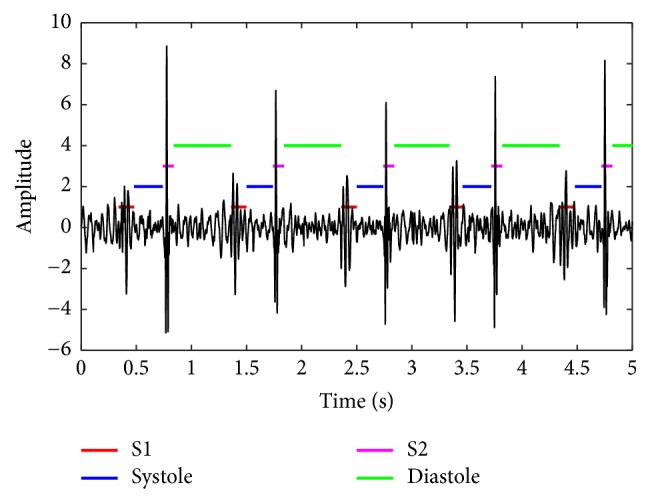
Illustration of the HSMM segmentation.
2.5. Features Extracted in Multidomains
2.5.1. Time-Domain Features (20 Features)
After the segmentation operation, a PCG recording is divided into many states in the order of S1, systole, S2, and diastole. The time interval of each state can be measured by the time difference between the beginning and the end. The cardiac cycle period can be measured by the time difference between the beginnings of two adjacent S1s. Since the intervals have physiological meanings in view point of heart physiology, Liu et al. [33] proposed 16 features from the intervals as shown in Table 1. Another 4 features from time-domain intervals are added in this paper.
Table 1.
Summary of time-domain features.
| Feature index | Feature name | Physical meaning |
|---|---|---|
| 1 | m_RR | mean value of RR intervals |
| 2 | sd_RR | standard deviation (SD) of RR intervals |
| 3 | m_IntS1 | mean value of S1 intervals |
| 4 | sd_IntS1 | SD of S1 intervals |
| 5 | m_IntS2 | mean value of S2 intervals |
| 6 | sd_IntS2 | SD of S2 intervals |
| 7 | m_IntSys | mean value of systolic intervals |
| 8 | sd_IntSys | SD of systolic intervals |
| 9 | m_IntDia | mean value of diastolic intervals |
| 10 | sd_IntDia | SD of diastolic intervals |
| 11 | m_Ratio_SysRR | mean value of the ratio of systolic interval to RR interval of each heart beat |
| 12 | sd_Ratio_SysRR | SD of the ratio of systolic interval to RR interval of each heart beat |
| 13 | m_Ratio_DiaRR | mean value of the ratio of diastolic interval to RR interval of each heart beat |
| 14 | sd_Ratio_DiaRR | SD of the ratio of diastolic interval to RR interval of each heart beat |
| 15 | m_Ratio_SysDia | mean value of the ratio of systolic to diastolic interval of each heart beat |
| 16 | sd_Ratio_SysDia | SD of the ratio of systolic to diastolic interval of each heart beat |
| 17 | m_Ratio_S1RR∗ | mean value of the ratio of S1 interval to RR interval of each heart beat |
| 18 | sd_Ratio_S1RR∗ | SD of the ratio of S1 interval to RR interval of each heart beat |
| 19 | m_Ratio_S2RR∗ | mean value of the ratio of S2 interval to RR interval of each heart beat |
| 20 | sd_Ratio_S2RR∗ | SD of the ratio of S2 interval to RR interval of each heart beat |
Note: ∗ means the new added features in this study.
2.5.2. Frequency Domain Features for States (77×4=308 Features)
Frequency spectrum is estimated for the S1 state of each cardiac cycle using a Gaussian window and discrete Fourier transform. The mean frequency spectrum over cycles can be further computed. The spectrum magnitudes from 30 Hz to 790 Hz with 10 Hz interval are taken as features. The maximum frequency 790 Hz is considered to adapt possible murmurs. So, 77 features for S1 state are obtained. Similar operation is done to S2, systole, and diastole state. So, the total number of features obtained from frequency domain for states is 77 features × 4 = 308 features.
2.5.3. Normalized Amplitude Features (12 Features)
Previous physiological findings in amplitude of heart sound [1–3] disclosed that the amplitude is related to heart hemodynamics. So, it is reasonable to extract features from amplitude of heart sounds. To eliminate the difference between subjects and records, no absolute amplitude is considered. Relative ratios of amplitude between states are extracted as given in Table 2.
Table 2.
Summary of normalized amplitude features.
| Feature index | Feature name | Physical meaning |
|---|---|---|
| 1 | m_Amp_SysS1 | mean value of the ratio of the mean absolute amplitude during systole to that during S1 in each heart beat |
| 2 | sd_Amp_SysS1 | SD of m_Amp_SysS1 |
| 3 | m_Amp_DiaS2 | mean value of the ratio of the mean absolute amplitude during diastole to that during S2 in each heart beat |
| 4 | sd_Amp_DiaS2 | SD of m_Amp_DiaS2 |
| 5 | m_Amp_S1S2 | mean value of the ratio of the mean absolute amplitude during S1 to that during S2 in each heart beat |
| 6 | sd_Amp_S1S2 | SD of m_Amp_S1S2 |
| 7 | m_Amp_S1Dia | mean value of the ratio of the mean absolute amplitude during S1 to that during diastole in each heart beat |
| 8 | sd_Amp_S1Dia | SD of m_Amp_S1Dia |
| 9 | m_Amp_SysDia | mean value of the ratio of the mean absolute amplitude during systole to that during diastole in each heart beat |
| 10 | sd_Amp_SysDia | SD of m_Amp_SysDia |
| 11 | m_Amp_S2Sys | mean value of the ratio of the mean absolute amplitude during S2 to that during systole in each heart beat |
| 12 | sd_Amp_S2Sys | SD of m_Amp_S2Sys |
2.5.4. Energy-Domain Features (47 Features)
The features in energy domain consist of two parts: the energy ratio of a band-pass signal to the original one and the energy ratio of one state to another.
For the first part, various frequency bands are considered with initial value of 10 Hz and increment bandwidth of 30 Hz; i.e., the 27 frequency bands are [10 40] Hz, [40 70] Hz, [70 100] Hz,…, and [790 820] Hz, respectively. The previous studies disclosed that murmurs' frequency is hardly higher than 800 Hz. In order to reflect murmurs' properties, the maximum frequency considered in this domain is 820 Hz. In this paper, each band-pass filter is designed by a five-order Butterworth filter. The output of the ith filter is yi:
| (1) |
where bi (numerator) and ai (denominator) are the Butterworth IIR filter coefficient vectors. Hence, the energy ratio is defined as
| (2) |
It is known that a normal heart sound signal generally has a frequency band blow 200 Hz. However, the frequency band may extend to 800 Hz if it contains murmurs. So, the energy ratio reflects signal energy distribution along frequency band. These features are helpful to discriminate a PCG records with murmurs or not.
For the second part, the relative energy ratio is investigated between any two states, resulting in another 20 features. The energy ratio of S1 to the cycle period is defined as
| (3) |
where N is the number of cycles in a PCG recording and n is the discrete time index. The authors consider average of Ratio_state_energyS1_cycle and standard deviation of Ratio_state_energyS1_cycle as two features. Similarly, another 18 features can be obtained from the averages and the standard deviations. The 47 proposed features in this domain are listed in Table 3.
Table 3.
Summary of energy-domain features.
| Feature index | Feature name | Physical meaning |
|---|---|---|
| 1-27 | Ratio_band_energyi | Ratio of a given band energy to the total energy |
| 28 | m_Ratio_state_energyS1_cycle | Mean of Ratio_state_energyS1_cycle |
| 29 | SD_Ratio_state_energyS1_cycle | standard deviation of Ratio_state_energyS1_cycle |
| 30 | m_Ratio_state_energyS2_cycle | Mean of Ratio_state_energyS2_cycle |
| 31 | SD_Ratio_state_energyS2_cycle | standard deviation of Ratio_state_energyS2_cycle |
| 32 | m_Ratio_state_energysys_cycle | Mean of Ratio_state_energysys_cycle |
| 33 | SD_Ratio_state_energysys_cycle | standard deviation of Ratio_state_energysys_cycle |
| 34 | m_Ratio_state_energydia_cycle | Mean of Ratio_state_energydia_cycle |
| 35 | SD_Ratio_state_energydia_cycle | standard deviation of Ratio_state_energydia_cycle |
| 36 | m_Ratio_state_energyS1_S2 | Mean of Ratio_state_energyS1_S2 |
| 37 | SD_Ratio_state_energyS1_S2 | standard deviation of Ratio_state_energyS1_S2 |
| 38 | m_Ratio_state_energyS1_sys | Mean of Ratio_state_energyS1_sys |
| 39 | SD_Ratio_state_energyS1_sys | standard deviation of Ratio_state_energyS1_sys |
| 40 | m_Ratio_state_energyS1_dia | Mean of Ratio_state_energyS1_dia |
| 41 | SD_Ratio_state_energyS1_dia | standard deviation of Ratio_state_energyS1_dia |
| 42 | m_Ratio_state_energyS2_sys | Mean of Ratio_state_energyS2_sys |
| 43 | SD_Ratio_state_energyS2_sys | standard deviation of Ratio_state_energyS2_sys |
| 44 | m_Ratio_state_energyS2_dia | Mean of Ratio_state_energyS2_dia |
| 45 | SD_Ratio_state_energyS2_dia | standard deviation of Ratio_state_energyS2_dia |
| 46 | m_Ratio_state_energydia_sys | Mean of Ratio_state_energydia_sys |
| 47 | SD_Ratio_state_energydia_sys | standard deviation of Ratio_state_energydia_sys |
2.5.5. Spectrum-Domain for Records Features (27 Features)
As is mentioned in Section 2.5.4, the frequency band is divided into 27 bands with start from 10 Hz to 30 Hz increment. Fast Fourier transform is performed for every record. The ratio of spectrum magnitude sum in a band to spectrum magnitude sum in whole band is taken as a feature. So, 27 features can be produced for a record. These features can discriminate murmurs because murmurs generally have higher frequency than those of normal heart sounds.
2.5.6. Cepstrum-Domain Features (13 Features × 5 = 65 Features)
The cepstrum of a PCG recording is calculated and the first 13 cepstral coefficients are taken as features [36]. Additionally, all S1 states from a PCG recording are joined together to create a new digital sequence. Then, the cepstrum can be calculated and the first 13 cepstral coefficients are taken as features. Similarly, the same operation is done to S2, systole, and diastole states. So, another 13 features × 3 = 39 features are obtained. The cepstrum of a signal p(n) is computed as follows:
| (4) |
| (5) |
| (6) |
where the operator DFT[.] is the discrete Fourier transform, IDFT[.] is the inverse DFT, log[.] is the natural logarithm, and |.| is the absolute operation. It is known that the cepstrum coefficient decays quickly. So, it is reasonable to select the first 13 coefficients as features. The cepstrum-domain features are listed in Table 4.
Table 4.
Summary of cepstrum-domain features.
| Feature index | Feature name | Physical meaning |
|---|---|---|
| 1-13 | Cepstrum coefficients | Cepstrum coefficients of a PCG recording |
| 14-26 | Cepstrum coefficients | Cepstrum coefficients of jointed S1 state |
| 27-39 | Cepstrum coefficients | Cepstrum coefficients of jointed systolic state |
| 40-52 | Cepstrum coefficients | Cepstrum coefficients of jointed S2 state |
| 53-65 | Cepstrum coefficients | Cepstrum coefficients of jointed diastole state |
2.5.7. Cyclostationary Features (4 Features)
(1) m_cyclostationarity_1 is mean value of the degree of cyclostationarity. The definition of “degree of cyclostationarity” can be found in [37]. This feature indicates the degree of a signal repetition. It will be infinite if the events which occurred in heart beating were exactly periodic. However, it will be a small number if the events are randomly alike. Let us assume γ(α) is the cycle frequency spectral density (CFSD) of a heart sound signal at cycle frequency α, as shown in Figure 3. This feature is defined as
| (7) |
where β is the maximum cycle frequency considered and η is the basic cycle frequency indicated by the main peak location of γ(α). A heart sound signal is equally divided into subsequences. The feature can be estimated for each subsequence; then the mean value and standard deviation can be obtained.
Figure 3.

An example of cycle frequency spectral density. (a) A subsequence of a PCG recording and (b) cycle frequency spectral density of the subsequence.
(2) sd_cyclostationarity_1 is SD of the degree of cyclostationarity.
(3) m_cyclostationarity_2 is mean value of the sharpness measure. The definition of this indicator is the sharpness of the peak of cycle frequency spectral density. It is
| (8) |
The operators max(.) and median(.) are the maximum and median magnitude of the cycle frequency spectral density. It is obvious that the sharper the peak is, the greater the feature is. Similarly, the feature can be calculated for each subsequence of the heart sound signal and then get the mean value and SD.
(4) sd_cyclostationarity_2 is SD of the sharpness measure.
The four features are listed in Table 5.
Table 5.
Summary of cyclostationary features.
| Feature index | Feature name | Physical Meaning |
|---|---|---|
| 1 | m_cyclostationarity_1 | mean value of the degree of cyclostationarity |
| 2 | sd_cyclostationarity_1 | SD of the degree of cyclostationarity |
| 3 | m_cyclostationarity_2 | mean value of the sharpness measure |
| 4 | sd_cyclostationarity_2 | SD of the sharpness measure |
2.5.8. High-Order Statistics Features (16 Features)
In probability theory and statistics, skewness is a measure of the asymmetry of the probability distribution of real-valued random numbers about its mean. It is a three-order statistics. Kurtosis is a measure of “tailedness” of the probability distribution of real-valued random numbers. It is a four-order statistics. The skewness and kurtosis of each state are considered here. There are sixteen related features, as listed in Table 6.
Table 6.
Summary of high-order statistics features.
| Feature index | Feature name | Physical Meaning |
|---|---|---|
| 1 | m_S1_skewness | mean value of the skewness of S1 |
| 2 | sd_S1_skewness | SD of the skewness of S1 |
| 3 | m_S1_kurtosis | mean value of the kurtosis of S1 |
| 4 | sd_S1_kurtosis | SD of the kurtosis of S1 |
| 5 | m_S2_skewness | mean value of the skewness of S2 |
| 6 | sd_S2_skewness | SD of the skewness of S2 |
| 7 | m_S2_kurtosis | mean value of the kurtosis of S2 |
| 8 | sd_S2_kurtosis | SD of the kurtosis of S2 |
| 9 | m_sys_skewness | mean value of the skewness of systole |
| 10 | sd_sys_skewness | SD of the skewness of systole |
| 11 | m_sys_kurtosis | mean value of the kurtosis of systole |
| 12 | sd_sys_kurtosis | SD of the kurtosis of systole |
| 13 | m_dia_skewness | mean value of the skewness of diastole |
| 14 | sd_dia_skewness | SD of the skewness of diastole |
| 15 | m_dia_kurtosis | mean value of the kurtosis of diastole |
| 16 | sd_dia_kurtosis | SD of the kurtosis of diastole |
2.5.9. Entropy Features (16 Features)
Sample entropy (SampEn) and fuzzy measure entropy (FuzzyMEn) have the ability to measure the complexity of a random sequence [38, 39]. Sample entropy and fuzzy measure entropy are both computed to measure the complexity of every state segmented by Springer's algorithm. Then, the average and standard deviation are used as the features. The detailed algorithm to calculate sample entropy and fuzzy measure entropy can be found in [38, 39]. So, 16 features in entropy are listed in Table 7.
Table 7.
Summary of entropy features.
| Feature index | Feature name | Physical meaning |
|---|---|---|
| 1 | m_SampEn_S1 | Mean value of SampEn of S1 state |
| 2 | SD_SampEn_S1 | SD value of SampEn of S1 state |
| 3 | m_SampEn_S2 | Mean value of SampEn of S2 state |
| 4 | SD_SampEn_S2 | SD value of SampEn of S2 state |
| 5 | m_SampEn_sys | Mean value of SampEn of systolic state |
| 6 | SD_SampEn_sys | SD value of SampEn of systolic state |
| 7 | m_SampEn_dia | Mean value of SampEn of diastolic state |
| 8 | SD_SampEn_dia | SD value of SampEn of diastolic state |
| 9 | m_FuzzyMEn_S1 | Mean value of FuzzyMEn of S1 state |
| 10 | SD_FuzzyMEn_S1 | SD value of FuzzyMEn of S1 state |
| 11 | m_FuzzyMEn_S2 | Mean value of FuzzyMEn of S2 state |
| 12 | SD_FuzzyMEn_S2 | SD value of FuzzyMEn of S2 state |
| 13 | m_FuzzyMEn_sys | Mean value of FuzzyMEn of systolic state |
| 14 | SD_FuzzyMEn_sys | SD value of FuzzyMEn of systolic state |
| 15 | m_FuzzyMEn_dia | Mean value of FuzzyMEn of diastolic state |
| 16 | SD_FuzzyMEn_dia | SD value of FuzzyMEn of diastolic state |
2.5.10. Summary
This paper considers 515 features in nine domains. They are listed in Table 8 for reference. To the authors' knowledge, the features extracted from entropy and cyclostationarity are new for heart sound classification. On the other hand, the combination of the features in the nine domains is novel for this classification. Seldom previous study has considered so many features simultaneously.
Table 8.
Summary of the proposed features.
| Index | Domain | Num. of features | Motivation |
|---|---|---|---|
| 1 | Time interval | 20 | The time interval of each state has physiological meaning based on heart physiology. |
| 2 | Frequency spectrum of state | 308 | To reflect the frequency spectrum within state. |
| 3 | State amplitude | 12 | The amplitude is related to the heart hemodynamics. |
| 4 | Energy | 47 | To reflect energy distribution with respect to frequency band |
| 5 | Frequency spectrum of records | 27 | To reflect frequency spectrum within records |
| 6 | Cepstrum | 65 | To reflect the acoustic properties. |
| 7 | Cyclostationary | 4 | To reflect the degree of signal repetition. |
| 8 | High-order statistics | 16 | To reflect the skewness and kurtosis of each signal state. |
| 9 | Entropy | 16 | To reflect the PCG signal inherent complexity. |
| Total | - - | 515 | - - |
2.6. SVM-Based Model for Signal Quality Estimation and Classification
The signal quality classification is typically two-category classification problem in this study. The SVM-based model has yielded excellent results in many two-class classification situations. Given a training sample set {xi, yi}, i = 1, ⋯, K, where xi is the feature vector xi ∈ Rd, yi is the label. So, SVM-based model is applicable for both signal quality estimation and classification. For the quality estimation, the label is yi ∈ {1,0}, which means good quality and bad quality. For the classification, the label is yi ∈ {1, −1}, which means abnormal and normal cases. The aim of SVM classifier is to develop optimal hyperplane between two classes besides distinguishing them. The optimal hyperplane can also be constructed by calculating the following optimization problem.
| (9) |
Here ξi is a relaxation variable and ξi ≥ 0, C is a penalty factor, and w is the coefficient vector. φ(xi) is introduced to get a nonlinear support vector machine. The optimization problem can be equally transformed into
| (10) |
where κ(xi, yi) is a kernel function. The authors use RBF kernel function in this paper. And the parameter sigma is empirically set as 14. The discussions about the selection of kernel function and the influence of sigma are given in the Section 4.3.
2.7. Scoring
The overall score is computed based on the number of records classified as normal, uncertain, or abnormal, in each of the reference categories. These numbers are denoted by Nnk, Nqk, Nak, Ank, Aqk, and Aak in Table 9.
Table 9.
Variables to evaluate the classification.
| Classification Results | ||||
|---|---|---|---|---|
| Normal (-1) | Uncertain (0) | Abnormal (1) | ||
| Reference label | Normal, clean | Nn 1 | Nq 1 | Na 1 |
| Normal, noisy | Nn 2 | Nq 2 | Na 2 | |
| Abnormal, clean | An 1 | Aq 1 | Aa 1 | |
| Abnormal, noisy | An 2 | Aq 2 | Aa 2 | |
Weights for the various categories are defined as follows (based on the distribution of the complete test set):
| (11) |
| (12) |
| (13) |
| (14) |
The modified sensitivity and specificity are defined as (based on a subset of the test set)
| (15) |
| (16) |
The overall score is then the average of these two values:
| (17) |
3. Results
3.1. Correlation Analysis between the Features and the Target Label
In this paper, a total of 515 features are extracted from a single recording. A question arises about how to evaluate the contribution of a feature for classification. To answer the question, correlation analysis is performed between the features and the target label. The correlation coefficients are plotted in the nine domains in Figure 4. The statistics of the coefficients are listed in Table 10. The top coefficient is 0.417 which is from “frequency spectrum of state” at 30 Hz of S2 state. This feature is called “top feature”. The statistics of top features are listed in Table 11. It is shown that 4 in the top 10 features are from “frequency spectrum of state”. So, this domain is ranked the first. Both “energy” and “entropy” contribute 3 in top 10. But “energy” contributes 12 in top 100 which is greater than “entropy” who contributes 8 in top 100. Therefore, “energy” is ranked the 2nd and “entropy” is ranked the 3rd. Following similar logics, the nine domains are ranked as shown in Table 11. It concludes that the domain “frequency spectrum of state” contributes the most. “Energy” and “entropy” are the second and third place to contribute.
Figure 4.

Correlation coefficient (CC) between features and the target label. (a) Time interval, (b) state amplitude, (c) energy, (d) high-order statistics, (e) cepstrum, (f) frequency spectrum of state, (g) cyclostationarity, (h) entropy, and (i) frequency spectrum of records.
Table 10.
Summary of the correlation coefficients.
| No. | Feature domain | Max. absolute CC |
Physical meaning |
|---|---|---|---|
| 1 | Time interval | 0.286 | sd_IntSys |
| 2 | State amplitude | -0.159 | sd_Amp_S2Sys |
| 3 | Energy | 0.345 | Standard deviation of Ratio_state_energydia_cycle |
| 4 | High-order statistics | 0.185 | sd_S1_kurtosis |
| 5 | Cepstrum | 0.216 | The seventh cepstrum coefficient of S2 state |
| 6 | Frequency spectrum of state | 0.417 | Spectrum value of 30 Hz of S2 state |
| 7 | cyclostationarity | -0.240 | Sharpness of the peak of cycle frequency spectral density |
| 8 | Entropy | -0.374 | Average value of sample entropy of diastolic state |
| 9 | Frequency spectrum of records | -0.272 | Ratio of spectrum magnitude sum in [90 120] Hz |
Table 11.
Rank order of the nine domains based on contribution.
| Rank order | Feature domain (Total num. of features) | Num. of top 10 features | Num. of top 100 features | Num. of top 200 features | Num. of top 300 features |
|---|---|---|---|---|---|
| 1 | Frequency spectrum of state (308) | 4 | 39 | 115 | 183 |
| 2 | Energy (47) | 3 | 12 | 16 | 24 |
| 3 | Entropy (16) | 3 | 8 | 10 | 11 |
| 4 | Cepstrum (65) | 0 | 14 | 28 | 40 |
| 5 | Time interval (20) | 0 | 14 | 17 | 17 |
| 6 | Frequency spectrum of records (27) | 0 | 5 | 5 | 10 |
| 7 | High-order statistics (16) | 0 | 4 | 4 | 7 |
| 8 | Cyclostationarity (4) | 0 | 2 | 3 | 4 |
| 9 | State amplitude (12) | 0 | 2 | 2 | 4 |
3.2. Signal Quality Estimation by SVM
The SVM model in (9) is used to discriminate signal quality. The reference labels for clean and noisy PCG recordings are “1” and “0”, respectively. The input to the model is the proposed 515 features. The performance is tested by various input, as shown in Table 12. Firstly, 10% of randomly selected data are used for training and the other 90% of data are used for testing without any overlap. Then the percent of train data increases by 10% and repeats. The performance summary for signal quality estimation is listed in Table 12. The manual reference indicates that there are 2874 clean recordings and 279 noisy recordings. So, the numbers of the two quality groups have great unbalance which has bad effect on network training. It is shown that the performance for good signal quality has excellent sensitivity from 96% to 98% no matter how much the percent of data for training varies from 10% to 90%. However, the performance for bad signal quality is poor. The specificity is around 50%; even the training data varies from 10% to 90%. Fortunately, this performance has little influence on the final classification, shown in the next subsection.
Table 12.
Performance of signal quality classification.
| Percent data to train | Percent data to test | Estimation results for Reference, clean |
Estimation results for Reference, noisy |
Sensitivity | Specificity | ||
|---|---|---|---|---|---|---|---|
| Clean | Noisy | Clean | Noisy | ||||
|
| |||||||
| 10% | 90% | 2421 | 166 | 104 | 146 | 0.96 | 0.47 |
| 20% | 80% | 2143 | 154 | 75 | 149 | 0.97 | 0.49 |
| 30% | 70% | 1869 | 143 | 59 | 136 | 0.97 | 0.49 |
| 40% | 60% | 1601 | 125 | 44 | 122 | 0.97 | 0.49 |
| 50% | 50% | 1332 | 104 | 36 | 104 | 0.97 | 0.50 |
| 60% | 40% | 1064 | 84 | 28 | 84 | 0.97 | 0.50 |
| 70% | 30% | 799 | 63 | 19 | 64 | 0.97 | 0.50 |
| 80% | 20% | 530 | 44 | 12 | 45 | 0.98 | 0.50 |
| 90% | 10% | 265 | 21 | 6 | 22 | 0.98 | 0.50 |
3.3. Classification of Normal/Abnormal by SVM
The classification of normal/abnormal is carried out by the SVM model as given in (9). The 515-feature vector is used as input to the SVM network and the label is used as output. The SVM model is firstly trained by a part of data and then tested by the other. To test the generation ability of the model, it is widely tested in following two cases.
Case 1 . —
All data (3153 recordings) are used to train the model and all data (3153 recordings) are to test the model. So, the training data and the testing data are fully overlapped.
Case 2 . —
10% of the normal recordings and 10% of the abnormal recordings are randomly selected to train the model, and the other 90% are to test the model. The training data and the testing data are exclusively nonoverlapped. This program independently repeats 200 times to evaluate the stability. Sensitivity and specificity are calculated in “mean±SD” to indicate the classification performance. Then, the percent of training data increases by 10%, the percent of test data decreases by 10%, and the evaluation process is repeated until the percent of training data reaches 90%.
The performance of the proposed classification is listed in Table 13. The overall score of Case 1 is up to 0.95. It proves that the proposed features are effective for this classification. In Case 2, it can be found that, with the increasing percent of data for training, both sensitivity and specificity increase. The standard deviation is not greater than 0.02. So, the score variation is very small; even the classifier independently runs 200 times. This simulation proves that the proposed features and the model have excellent generation ability and stability and are effective in discriminating the PCG recordings.
Table 13.
Performance of the classification.
| Case | Percent of data to train | Percent of data to test | Repeat times | Training and test data division | Sensitivity | Specificity | Overall score |
|---|---|---|---|---|---|---|---|
| Case 1 | 100% | 100% | 1 | No | 0.99 | 0.91 | 0.95 |
|
| |||||||
| Case 2 | 10% | 90% | 200 | Yes | 0.68±0.06 | 0.87±0.03 | 0.77±0.02 |
| 20% | 80% | 200 | Yes | 0.76±0.05 | 0.86±0.02 | 0.81±0.02 | |
| 30% | 70% | 200 | Yes | 0.80±0.04 | 0.87±0.02 | 0.83±0.02 | |
| 40% | 60% | 200 | Yes | 0.82±0.04 | 0.87±0.01 | 0.85±0.02 | |
| 50% | 50% | 200 | Yes | 0.84±0.03 | 0.87±0.01 | 0.85±0.01 | |
| 60% | 40% | 200 | Yes | 0.85±0.04 | 0.87±0.01 | 0.86±0.01 | |
| 70% | 30% | 200 | Yes | 0.86±0.04 | 0.87±0.01 | 0.87±0.02 | |
| 80% | 20% | 200 | Yes | 0.87±0.04 | 0.87±0.02 | 0.87±0.02 | |
| 90% | 10% | 200 | Yes | 0.88±0.04 | 0.87±0.02 | 0.88±0.02 | |
Note: the number is presented as mean±SD.
4. Discussions
4.1. Effect of the Number of Top Features
This paper proposes 515 features from multidomains. However, correlation analysis shows that each feature has different degree of correlation with the target label. The performance will change with the number of selected features. To evaluate the effect of selected features, the authors conduct simulations under condition of varying the top number of features. The mean overall score changing with respect to the number of top features is illustrated in Figure 5, where Figure 5(a) shows the performance with top 1 to top 5 features, Figure 5(b) is with top 10 to top 50 features, and Figure 5(c) is with top 100 to top 515 features. It can be seen that there are two factors to influence SVM classifier's generalization ability. One is the percent of data for training; the other is the number of top features. An overall look shows that both the two factors have positive effect on the classification performance. Roughly speaking, if any one of them increases, the performance will get improvement. However, it is not always true. A closer look at Figure 5(a) indicates the performance has little change as the percent increases. But the performance gets much improvement as the percent increases, shown in Figures 5(b) and 5(c), where the number of top features is much greater than that in Figure 5(a). A careful look at Figure 5(c) discloses that the case that all the features (515) are involved does not result in the best performance. It can be found that there is an “edge effect” on the selection of top feature number. That is, much improvement can be obtained via increasing top feature number as the number is small. However, the improvement becomes little when the number is up to some degree. The best performance is obtained with top 400 features in this paper. The performance will get worse if the number continues to increase.
Figure 5.

Classification performance with respect to the number of top features and percent of data for training. (a) Overall scores obtained by top 1, top 2, top 3, top 4, and top 5 features. (b) Overall scores obtained by top 10, top 20, top 30, top 40, and top 50 features. (c) Overall scores obtained by top 100, top 200, top 300, top 400, and top 515 features.
The proposed classification has very good performance even if the number of features is small. For example, it can be noted in Figure 5(a) that the overall score is up to 0.71 as only the top 1 feature is used and the score increases to 0.81 when the top 10 features are used. This is one of attractive advantages of the proposed classification.
Another advantage is that the proposed SVM classifier has very stable output. Even if the SVM classifier is trained independently by randomly selected features, the overall score has very low variations (standard variance is approximately lower than 0.02). That is to say, the proposed features and SVM classifier are adaptable to the classification.
4.2. Classification Performance Based on Features in Specified Domain
Table 13 and Figure 5 show the classification performance based on mixed features from multidomains. It is interesting to test the performance based on features of a separated domain. This test would be evidence to show the power of combined features for classification. So, the SVM classifier and 10-fold validation are used for this purpose. The results are listed in Table 14. It is seen that, the highest score, 0.85, is produced if only the features in “frequency spectrum of state” are used. Other high scores are obtained based on features in domain of “entropy”, “energy”, and “cepstrum”. It can be found that these results are almost coincident with those of correlation analysis given in Section 3.1 where “frequency spectrum of state”, “energy”, “entropy”, and “cepstrum” are the top domains to contribute effective features. This simulation indicates that it is reasonable to improve classification performance by combining multidomain features.
Table 14.
Classification performance based on features in specified domain.
| Rank | Domain (# features) | Mean of overall score | Standard deviation |
|---|---|---|---|
| 1 | Frequency spectrum of state (308) | 0.85 | 0.021 |
| 2 | Entropy (16) | 0.82 | 0.028 |
| 3 | Energy (47) | 0.78 | 0.020 |
| 4 | Cepstrum (65) | 0.75 | 0.027 |
| 5 | High-order statistics (16) | 0.73 | 0.029 |
| 6 | Frequency spectrum of records (27) | 0.71 | 0.025 |
| 7 | Time interval (20) | 0.70 | 0.025 |
| 8 | Cyclostationarity (4) | 0.65 | 0.042 |
| 9 | State amplitude (12) | 0.61 | 0.025 |
4.3. Selection of Kernel Function and Influence of the Gaussian Kernel Function
Typically, the kernel functions for a SVM have several selections, such as linear kernel, polynomial kernel, sigmoid kernel, and Gaussian radial basis function. Given an arbitrary dataset, one does not know which kernel may work best. Generally, one can start with the simplest hypothesis space first and then work a way up towards a more complex hypothesis space. The authors followed this lesson summarized by the previous researchers. A bad performance was produced by the SVM classifier using a linear kernel since 515 features in this study were complex and they were not linearly separable, as well as using a polynomial kernel. The authors actually tried out all possible kernels and found that the RBF kernel produced the best performance. The authors believed that the best performance should be attributed to the RBF kernel's advantages. The first is translation invariance. Let the RBF kernel be K(xi, xj) = exp(−‖xi − xj‖/γ); then K(xi, xj) = K(xi + ν, xj + ν) where ν is any arbitrary vector. It is known that the kernel is effectively a similarity measure. The invariance is useful to measure the similarity between the proposed features. The second is that the similarity is measured by Euclidean distance. RBF kernel is a function of the Euclidean distance between the features. In this study, the Euclidean distance is a preferred similarity metric. The authors selected the RBF kernel function because the advantages match the classification purpose and features.
One difficulty with the Gaussian RBF kernel function is the parameter sigma governing the kernel width. A general conclusion about sigma has been summarized by previous researchers. A large value of sigma may lead to an over smoothing hyperplane and a washing out of structure that might otherwise be extracted from the feature space. A reducing value of sigma may lead to a noisy hyperplane elsewhere in the feature space where the feature density is smaller. There is a trade-off between sensitivity to noise at small value and over smoothing at large value. To select appropriate value for sigma, the authors did grid search in a specified range, as seen in Figure 6. This figure shows the mean overall score, based on 50 independent runs, with respect to rate of data for training and value of sigma where the value of sigma increases from 4 to 35 by step of 1 and the rate of data for training increases from 0.1 to 0.9 by step of 0.1. It is found that the peak of the overall score occurs at sigma 14 as indicated by the diamond.
Figure 6.
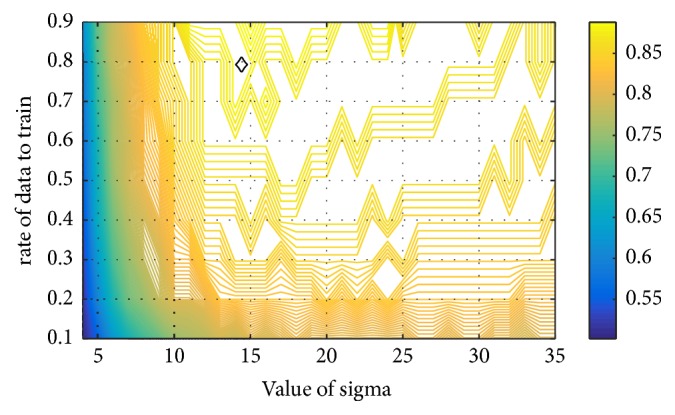
The mean overall score with respect to rate of data for training and value of sigma. The diamond shows the peak position.
5. Conclusions
In this paper, 515 features are extracted from multiple domains, i.e., time interval, state amplitude, energy, high-order statistics, cepstrum, frequency spectrum, cyclostationarity, and entropy. Correlation analysis between the features and the target label shows that the features from frequency spectrum contribute the most to the classification. The features and the SVM classifier jointly show the powerful classification performance. The results show the overall score reaches 0.88±0.02 based on 200 independent simulations, which is competitive to the previous best classification methods. Moreover, the SVM classifier has very good performance with even small number of features for training and has stable output regardless of randomly selected features for training.
Acknowledgments
This work was supported in part by the National Natural Science Foundation of China under Grants no. 61471081 and no. 61601081 and Fundamental Research Funds for the Central Universities under Grant nos. DUT15QY60, DUT16QY13, DC201501056, and DCPY2016008.
Contributor Information
Hong Tang, Email: tanghong@dlut.edu.cn.
Chengyu Liu, Email: bestlcy@sdu.edu.cn.
Data Availability
The authors state that the data used in this study are available from the website http://www.physionet.org/challenge/2016/ to support the conclusions.
Conflicts of Interest
The authors declare that there are no conflicts of interest regarding the publication of this paper.
References
- 1.Luisada A. A., Liu C. K., Aravanis C., Testelli M., Morris J. On the mechanism of production of the heart sounds. American Heart Journal . 1958;55(3):383–399. doi: 10.1016/0002-8703(58)90054-1. [DOI] [Google Scholar]
- 2.Sakamoto T., Kusukawa R., Maccanon D. M., Luisada A. A. Hemodynamic determinants of the amplitude of the first heart sound. Circulation Research. 1965;16:45–57. doi: 10.1161/01.res.16.1.45. [DOI] [PubMed] [Google Scholar]
- 3.Sakamoto T., Kusukawa R., MacCanon D. M., Luisada A. A. First heart sound amplitude in experimentally induced alternans. CHEST. 1966;50(5):470–475. doi: 10.1378/chest.50.5.470. [DOI] [PubMed] [Google Scholar]
- 4.Durand L.-G., Pibarot P. Digital signal processing of the phonocardiogram: Review of the most recent advancements. Critical Reviews in Biomedical Engineering. 1995;23(3-4):163–219. doi: 10.1615/CritRevBiomedEng.v23.i3-4.10. [DOI] [PubMed] [Google Scholar]
- 5.Gerbarg D. S., Taranta A., Spagnuolo M., Hofler J. J. Computer analysis of phonocardiograms. Progress in Cardiovascular Diseases. 1963;5(4):393–405. doi: 10.1016/S0033-0620(63)80007-9. [DOI] [Google Scholar]
- 6.Akay Y., Akay M., Welkowitz W., Kostis J. Noninvasive detection of coronary artery disease. IEEE Engineering in Medicine and Biology Magazine. 1994;13(5):761–764. doi: 10.1109/51.334639. [DOI] [PubMed] [Google Scholar]
- 7.Durand L.-G., Blanchard M., Cloutier G., Sabbah H. N., Stein P. D. Comparison of Pattern Recognition Methods for Computer-Assisted Classification of Spectra of Heart Sounds in Patients with a Porcine Bioprosthetic Valve Implanted in the Mitral Position. IEEE Transactions on Biomedical Engineering. 1990;37(12):1121–1129. doi: 10.1109/10.64456. [DOI] [PubMed] [Google Scholar]
- 8.Uğuz H. A biomedical system based on artificial neural network and principal component analysis for diagnosis of the heart valve diseases. Journal of Medical Systems. 2012;36(1):61–72. doi: 10.1007/s10916-010-9446-7. [DOI] [PubMed] [Google Scholar]
- 9.Ölmez T., Dokur Z. Classification of heart sounds using an artificial neural network. Pattern Recognition Letters. 2003;24(1–3):617–629. doi: 10.1016/s0167-8655(02)00281-7. [DOI] [Google Scholar]
- 10.Dokur Z., Ölmez T. Heart sound classification using wavelet transform and incremental self-organizing map. Digital Signal Processing. 2008;18(6):951–959. doi: 10.1016/j.dsp.2008.06.001. [DOI] [Google Scholar]
- 11.Ari S., Hembram K., Saha G. Detection of cardiac abnormality from PCG signal using LMS based least square SVM classifier. Expert Systems with Applications. 2010;37(12):8019–8026. doi: 10.1016/j.eswa.2010.05.088. [DOI] [Google Scholar]
- 12.Maglogiannis I., Loukis E., Zafiropoulos E., Stasis A. Support Vectors Machine-based identification of heart valve diseases using heart sounds. Computer Methods and Programs in Biomedicine. 2009;95(1):47–61. doi: 10.1016/j.cmpb.2009.01.003. [DOI] [PubMed] [Google Scholar]
- 13.Zheng Y., Guo X., Ding X. A novel hybrid energy fraction and entropy-based approach for systolic heart murmurs identification. Expert Systems with Applications. 2015;42(5):2710–2721. doi: 10.1016/j.eswa.2014.10.051. [DOI] [Google Scholar]
- 14.Bentley P. M., Grant P. M., McDonnell J. T. E. Time-frequency and time-scale techniques for the classification of native and bioprosthetic heart valve sounds. IEEE Transactions on Biomedical Engineering. 1998;45(1):125–128. doi: 10.1109/10.650366. [DOI] [PubMed] [Google Scholar]
- 15.Avendaño-Valencia L. D., Godino-Llorente J. I., Blanco-Velasco M., Castellanos-Dominguez G. Feature extraction from parametric time-frequency representations for heart murmur detection. Annals of Biomedical Engineering. 2010;38(8):2716–2732. doi: 10.1007/s10439-010-0077-4. [DOI] [PubMed] [Google Scholar]
- 16.Quiceno-Manrique A. F., Godino-Llorente J. I., Blanco-Velasco M., Castellanos-Dominguez G. Selection of dynamic features based on time-frequency representations for heart murmur detection from phonocardiographic signals. Annals of Biomedical Engineering. 2010;38(1):118–137. doi: 10.1007/s10439-009-9838-3. [DOI] [PubMed] [Google Scholar]
- 17.Yang T., Hsieh H. Classification of Acoustic Physiological Signals Based on Deep Learning Neural Networks with Augmented Features. Proceedings of the 43rd Computing in Cardiology Conference; 2016; Vancouver, Canada. [DOI] [Google Scholar]
- 18.Tschannen M., Kramer T., Marti G., Heinzmann M., Wiatowski T. Heart sound classification using deep structured features. Proceedings of the 43rd Computing in Cardiology Conference, CinC 2016; September 2016; Vancouver, Canada. pp. 565–568. [Google Scholar]
- 19.Nilanon T., Yao J., Hao J., Purushotham S., Liu Y. Normal / abnormal heart sound recordings classification using convolutional neural network. Proceedings of the 43rd Computing in Cardiology Conference, CinC 2016; September 2016; Vancouver, Canada. pp. 585–588. [Google Scholar]
- 20.Diaz Bobillo I. A Tensor Approach to Heart Sound Classification. Proceedings of the 2016 Computing in Cardiology Conference; 2016; Vancouver, Canada. [DOI] [Google Scholar]
- 21.Bouril A., Aleinikava D., Guillem M. S., Mirsky G. M. Automated classification of normal and abnormal heart sounds using support vector machines. Proceedings of the 43rd Computing in Cardiology Conference, CinC 2016; September 2016; Vancouver, Canada. pp. 549–552. [Google Scholar]
- 22.Gonzalez Ortiz J. J., Phoo C. P., Wiens J. Heart Sound Classification Based on Temporal Alignment Techniques. Proceedings of the 2016 Computing in Cardiology Conference; 2016; Vancouver, Canada. [DOI] [Google Scholar]
- 23.Nabhan Homsi M., Medina N., Hernandez M., et al. Automatic Heart Sound Recording Classification using a Nested Set of Ensemble Algorithms. Proceedings of the 2016 Computing in Cardiology Conference; 2016; Vancouver, Canada. [DOI] [Google Scholar]
- 24.Langley P., Murray A. Heart sound classification from unsegmented phonocardiograms. Physiological Measurement. 2017;38(8):1658–1670. doi: 10.1088/1361-6579/aa724c. [DOI] [PubMed] [Google Scholar]
- 25.Nabhan Homsi M., Warrick P. Ensemble methods with outliers for phonocardiogram classification. Physiological Measurement. 2017;38(8):1631–1644. doi: 10.1088/1361-6579/aa7982. [DOI] [PubMed] [Google Scholar]
- 26.Whitaker B., Anderson D. Heart Sound Classification via Sparse Coding. Proceedings of the 43rd Computing in Cardiology Conference; 2016; Vancouver, Canada. [DOI] [Google Scholar]
- 27.Whitaker B. M., Suresha P. B., Liu C., Clifford G. D., Anderson D. V. Combining sparse coding and time-domain features for heart sound classification. Physiological Measurement. 2017;38(8):1701–1713. doi: 10.1088/1361-6579/aa7623. [DOI] [PubMed] [Google Scholar]
- 28.Potes C., Parvaneh S., Rahman A., Conroy B. Ensemble of feature-based and deep learning-based classifiers for detection of abnormal heart sounds. Proceedings of the 43rd Computing in Cardiology Conference, CinC 2016; September 2016; Vancouver, Canada. pp. 621–624. [Google Scholar]
- 29.Zabihi M., Bahrami Rad A., Kiranyaz S., Gabbouj M., K. Katsaggelos A. Heart Sound Anomaly and Quality Detection using Ensemble of Neural Networks without Segmentation. 43rd Computing in Cardiology Conference; 2016; Vancouver, Canada. [DOI] [Google Scholar]
- 30.Kay E., Agarwal A. DropConnected Neural Network Trained with Diverse Features for Classifying Heart Sounds. Proceedings of the 43rd Computing in Cardiology Conference; 2016; Vancouver, Canada. [DOI] [Google Scholar]
- 31.Tang H., Chen H., Li T., Zhong M. Classification of Normal/Abnormal Heart Sound Recordings based on Multi:Domain Features and Back Propagation Neural Network. Proceedings of the 43rd Computing in Cardiology Conference; 2016; Vancouver, Canada. [DOI] [Google Scholar]
- 32. http://www.physionet.org/challenge/2016/, Nov. 16, 2016.
- 33.Liu C., Springer D., Li Q., et al. An open access database for the evaluation of heart sound algorithms. Physiological Measurement. 2016;37(12):2181–2213. doi: 10.1088/0967-3334/37/12/2181. [DOI] [PMC free article] [PubMed] [Google Scholar]
- 34.Schmidt S. E., Holst-Hansen C., Graff C., Toft E., Struijk J. J. Segmentation of heart sound recordings by a duration-dependent hidden Markov model. Physiological Measurement. 2010;31(4):513–529. doi: 10.1088/0967-3334/31/4/004. [DOI] [PubMed] [Google Scholar]
- 35.Springer D. B., Tarassenko L., Clifford G. D. Logistic regression-HSMM-based heart sound segmentation. IEEE Transactions on Biomedical Engineering. 2016;63(4):822–832. doi: 10.1109/TBME.2015.2475278. [DOI] [PubMed] [Google Scholar]
- 36.Boucheron L. E., De Leon P. L., Sandoval S. Low bit-rate speech coding through quantization of mel-frequency cepstral coefficients. IEEE Transactions on Audio, Speech and Language Processing. 2012;20(2):610–619. [Google Scholar]
- 37.Li T., Tang H., Qiu T., Park Y. Best subsequence selection of heart sound recording based on degree of sound periodicity. IEEE Electronics Letters. 2011;47(15):841–843. doi: 10.1049/el.2011.1693. [DOI] [Google Scholar]
- 38.Liu C., Li K., Zhao L., et al. Analysis of heart rate variability using fuzzy measure entropy. Computers in Biology and Medicine. 2013;43(2):100–108. doi: 10.1016/j.compbiomed.2012.11.005. [DOI] [PubMed] [Google Scholar]
- 39.Zhao L., Wei S., Zhang C., et al. Determination of sample entropy and fuzzy measure entropy parameters for distinguishing congestive heart failure from normal sinus rhythm subjects. Entropy. 2015;17(9):6270–6288. doi: 10.3390/e17096270. [DOI] [Google Scholar]
Associated Data
This section collects any data citations, data availability statements, or supplementary materials included in this article.
Data Availability Statement
The authors state that the data used in this study are available from the website http://www.physionet.org/challenge/2016/ to support the conclusions.