A computational strategy to adjust for copy number in tumor Hi-C data

Abstract

Motivation: The Hi-C technology was designed to decode the three-dimensional conformation of the genome. Despite progress towards more and more accurate contact maps, several systematic biases have been demonstrated to affect the resulting data matrix. Here we report a new source of bias that can arise in tumor Hi-C data, which is related to the copy number of genomic DNA. To address this bias, we designed a chromosome-adjusted iterative correction method called caICB. Our caICB correction method leads to significant improvements when compared with the original iterative correction in terms of eliminating copy number bias.

Availability and Implementation: The method is available at https://bitbucket.org/mthjwu/hicapp.

Contact: michor@jimmy.harvard.edu

Supplementary information: Supplementary data are available at Bioinformatics online.

1 Introduction

Our knowledge of the higher-order structure of the genome has rapidly expanded over the last decade with the development of several methods able to elucidate the non-linear spatial conformation of the genome (Fullwood et al., 2010; Kalhor et al., 2012; Lieberman-Aiden et al., 2009). One important contribution was the development of a chromatin conformation capture-based method called Hi-C (Lieberman-Aiden et al., 2009), which enables high-throughput analysis of spatial structures of chromatin. Recent improvements of the Hi-C protocol led to a characterization of chromatin structure from many species at increased resolution (Dixon et al., 2012, 2015; Jin et al., 2013; Le et al., 2013; Lieberman-Aiden et al., 2009; Nagano et al., 2013; Naumova et al., 2013; Rao et al., 2014), from the original 1 Mb map (Lieberman-Aiden et al., 2009) to the most recent 1 Kb map (Rao et al., 2014).

Increasing effort has since been devoted to studies of the biological function and consequences of the 3D chromatin architecture, such as its role in promoter-enhancer regulation (Jin et al., 2013) and associations between chromatin conformation and DNA replication timing (De and Michor, 2011; Fudenberg et al., 2011; Pope et al., 2014) as well as local mutation rates (Liu et al., 2013). Hi-C data at different resolutions may enable researchers to infer different levels of genomic interactions; for instance, a 1 Mb resolution elucidates the overall folding principles of chromosomes, which were found to be consistent among different cell types within each species (Lieberman-Aiden et al., 2009); a 50–100 Kb resolution provides chromosome domain information which is associated with histone marks (Dixon et al., 2012; Huang et al., 2015); and a 1–10 kb resolution enables detailed studies of chromatin looping, such as enhancer–promoter or enhancer–enhancer interactions, which can be specific to different cell types (Jin et al., 2013; Rao et al., 2014).

Raw Hi-C data hve been observed to have both technical and biological biases (Yaffe and Tanay, 2011), with three predominant sources of bias identified so far: fragment length, GC bias and mappability. To correct for these biases, many software packages have been developed in order to generate an unbiased interaction map (Ay and Noble, 2015; Hu et al., 2012; Imakaev et al., 2012; Li et al., 2015; Sauria et al., 2015; Servant et al., 2012; Shavit and Lio, 2014; Yaffe and Tanay, 2011). Hicpipe (Yaffe and Tanay, 2011) and hicnorm (Hu et al., 2012) are explicit correction methods which fit probabilistic and regression models, respectively, to normalize the raw Hi-C map. These approaches require a priori knowledge of the biases. Another method, used in software such as Hiclib (Imakaev et al., 2012) and HiCorrector (Li et al., 2015), performs an iterative correction (IC), which does not require a priori knowledge of the biases. Such methods use a matrix balancing or scaling algorithm (Knight and Ruiz, 2013; Sinkhorn and Knopp, 1967) to iteratively correct for all possible biases, based on the assumption that all loci should have equal representation in the data if there is no bias. IC-based methods generate a bias vector defined as IC bias (ICB, denoted as B below) that converts the raw matrix (R) to a normalized matrix (N_ij = B_iB_jR_ij in which i and j represent two genomic loci). Because of ease of application and high running speed, easy transformation between the raw and normalized matrices and no requirement of the explicit information on biases, IC-based methods (also called ICB correction) have become the most widely used Hi-C normalization approaches that can correct for both known and unknown biases in many current applications (Rao et al., 2014).

A novel source of bias that can arise in Hi-C data is related to the copy number of genomic material. This type of bias has so far been unaccounted for since most Hi-C applications investigate normal tissue and healthy cell line samples, which have mostly uniform copy numbers of chromosomes. However, once tumor samples are analyzed, biases related to copy number alterations become important and need to be corrected for in order to obtain an accurate view of the interaction map between genomic locations. So far, limited Hi-C experiments have been carried out on tumor samples (Barutcu et al., 2015; Rao et al., 2014; Rickman et al., 2012). For a genome with non-uniform copy number, such as that of tumor cells, DNA copy number variation can introduce critical bias in Hi-C data because genomic locations with a higher copy number have a greater chance to be sequenced in the Hi-C protocol, and genomic locations with low copy number might not be detected at all in Hi-C data.

We first identified the bias caused by DNA copy number by analyzing the ENCODE K562 Hi-C data (Rao et al., 2014). Surprisingly, we found that the copy number bias still existed after within-chromosome ICB correction (Li et al., 2015). Further analyses demonstrated that the ICB method can correct for copy number biases within each chromosome but not between chromosomes, which also cannot be adjusted for simply by using total or average contact counts of chromosomes. By utilizing the count-distance curve between the contact counts and the genomic distance between the contact pairs, we converted the problem of removing the biases across chromosomes to the problem of minimizing the differences across count-distance curves of different chromosomes. We thus designed a linear regression-based chromosome-level adjustment method called caICB, which is based on the ICB protocol, to correct for this bias. We performed the analyses on multiple resolution contact maps (1 Mb, 250, 100 and 10 Kb) and found that the performance of our caICB correction is significantly better than the original ICB method in terms of correcting for copy number biases. Our analyses show that the three previously identified bias factors are also accurately corrected for by caICB. Furthermore, the caICB correction is robust when using a small subset of genomic ranges instead of using the whole genome contact map, and is easy and fast to apply even for extremely high-resolution maps. Our method does not require copy number data for the samples for which Hi-C data are available, and has the potential to adjust for other biases in Hi-C data without a priori knowledge.

2 Methods

We evaluated copy number as well as fragment length, GC content and mappability biases in Hi-C data of the K562 cancer cell line. The raw contact counts in 1 Mb, 250 Kb, 100 Kb and 10 Kb resolution Hi-C maps were obtained from GEO with accession number GSE63525 (Rao et al., 2014). The maps had already been pre-processed to remove experimental artifacts. The ICBwas then determined using HiCorrector (Li et al., 2015) for 30 iterations within each chromosome. Different subsets of genomic ranges were considered to study the bias effects in K562 Hi-C data (Supplementary Fig. S1). We also applied our method to MCF7 Hi-C data (Barutcu et al., 2015) for 1 Mb and 250 Kb resolutions. The raw fastq files were downloaded from GEO with accession number GSE66733 (Barutcu et al., 2015). HiCup (Wingett, et al., 2015) was used to pre-process the data to remove experimental artifacts, which resulted in interaction maps with 1 Mb and 250 Kb resolution. The subsequent processing steps were the same as above.

2.1 Spline model

A significant drop in contact counts was observed with increasing genomic distance between two loci of the same chromosome in all published Hi-C datasets. Because of the different Hi-C protocol settings, it is difficult to identify a single function that can capture the relationship between contact counts and genomic distance (Ay et al., 2014). Thus, in previous studies (Ay et al., 2014; Dixon et al., 2012; Jin et al., 2013; Rao et al., 2014), local regression methods such as loess or spline were employed to capture this relationship. In our analysis, we used spline implemented as the R function ‘smooth.spline’ (http://www.bioconductor.org/) to capture the relationship. First, the mean contact counts (o_i) among all locus pairs with the same genomic distance (d_i) were calculated by removing extreme data points that are outside of a 10-fold of interquantile range (IQR). Then spline models were fit to the resulting o_i and d_i pairs to capture the expected contact counts for different genomic distances. The analyses were performed on raw data, ICB-corrected and caICB-corrected data (see below) of different resolutions in order to calculate the observed/expected (O/E) values in different conditions. The O/E values were then used to evaluate the results of different normalization strategies.

2.2 Linear model to correct for ICB

By utilizing the count-distance curve between the contact counts and the genomic distance between the contact pairs, we converted the problem of removing the biases across chromosomes to the problem of minimizing the differences across count-distance curves of different chromosomes. We assumed that the mean contact counts of the same genomic distances for different chromosomes are the same if no bias were observed in the Hi-C data. We propose a linear regression-based method to minimize the differences between count-distance curves of different chromosomes, which can correct for the across-chromosome bias without changing the within chromosome bias structure learned from ICB correction step. Specifically, the mean (ICB-corrected) contact counts (Oi|j, i = 2, ., K) among all locus pairs with the same genomic distance (di|j, i = 2, ., K) in each chromosome j (j = 1, ., N) were calculated by removing the extreme data points that were outside of a 10-fold IQR. Genomic distance between locus pairs was calculated by

$$d_{i|j}=r\mathrm{ }\times \mathrm{ }i, i=2,.,K,$$

where r is the resolution of the Hi-C map, i is the binning step between locus pairs, j is the chromosome index and K is the tuning parameter controlling the number of adjacent interaction bins from each genomic locus chosen for the correction. This parameter represents the tradeoff between accuracy and efficiency, since larger values of K include more data points, which reduces efficiency but increases accuracy, and vice versa. K equals to 200 was used in all analyses in this study. Then linear regression on Oi|j between every chromosome pair was performed as follows:

$$E\left(O_{i|m}\right)=\mathrm{ }{\mathrm{\beta }}_{m,n}\times O_{i|n}, m\in j,\mathrm{ }n\in j,$$

$\mathrm{w}\mathrm{h}\mathrm{e}\mathrm{r}\mathrm{e}\mathrm{ }E\left(O_{i|m}\right)$ is the linear estimation of $O_{i|m}$ from $O_{i|n}$, and the coefficient ${\mathrm{\beta }}_{m,n}$ represents the bias between chromosomes m and n. This step was taken to calculate the coefficient matrix ($B_{m\hspace{0.5em}\times \hspace{0.5em}n},\mathrm{ }m\in j,\mathrm{ }n\in j$) representing the biases between each chromosome pair.$B_{m\hspace{0.5em}\times \hspace{0.5em}n}$ is a m × n matrix with elements ${\mathrm{\beta }}_{m,n}$.The matrix $B_{m\hspace{0.5em}\times \hspace{0.5em}n}$ was further standardized by dividing with coefficients from chromosome 1:

$${\mathrm{\beta }}_{m,n}^{\mathrm{\text{'}}}=\frac{{\mathrm{\beta }}_{m,n}}{{\mathrm{\beta }}_{m,1}}$$

Then cbias was learned as the square root of the median standardized coefficients of each chromosome:

$${\mathrm{c}\mathrm{b}\mathrm{i}\mathrm{a}\mathrm{s}}_{\mathrm{c}}=\sqrt{\mathrm{m}\mathrm{e}\mathrm{d}\mathrm{i}\mathrm{a}\mathrm{n}\left({\mathrm{\beta }}_{m,n}^{\mathrm{\text{'}}}\right)},\mathrm{ }n=1,\mathrm{ }2,\mathrm{ }\dots ,\mathrm{ }N,\mathrm{ }m\in j,\mathrm{ }c\in j.$$

Finally, caICB was calculated from ICB by correcting for the chromosome level bias (cbias) by applying

$${\mathrm{c}\mathrm{a}\mathrm{I}\mathrm{C}\mathrm{B}}_{\mathrm{c}}^{\mathrm{b}}={\mathrm{I}\mathrm{C}\mathrm{B}}_{\mathrm{c}}^{\mathrm{b}}\mathrm{ }\times \mathrm{ }{\mathrm{c}\mathrm{b}\mathrm{i}\mathrm{a}\mathrm{s}}_{\mathrm{c}}$$

The caICB correction ideally accounts for all biases in the Hi-C data, and was used to normalize the raw count matrix to generate a corrected Hi-C map, or alternatively can be used in the Fit-Hi-C package (Ay et al., 2014) to obtain an unbiased list of significant contacts. The caICB correction algorithm was implemented in the HiCapp Hi-C analysis pipeline, which can be obtained from https://bitbucket.org/mthjwu/hicapp. The implementation of our caICB correction includes and extends the ICB correction, which can correct for both within- and across-chromosome copy number biases as well as other potential biases in raw Hi-C maps of any given resolution.

2.3 Calculation of explicit biases

Segmentation results of snp6.0 microarray data of all available tumor cell lines were obtained from the CCLE project website (Barretina et al., 2012). Log2 copy number, which is the log2 ratio of the tumor sample intensity to the normal sample intensity, of the genomic bins in different resolutions was calculated from segmentation results by using the DNAcopy package in bioconductor (Seshan and Olshen, 2016). The log2 multiplicative copy number was calculated by adding the log2 copy numbers of the two genomic bins of each locus pair. In silico restriction enzyme cutting of the hg19 version of the human genome was performed by using the ‘hiccup_digester’ script from the HiCUP package (Wingett et al., 2015); fragment length was then obtained from the in silico cutting results. Surrounding sequences of 200 and 500 bp around each restriction enzyme cutting site were used to calculate the GC content and mappability scores, respectively. The fragment-based score was determined by averaging the scores of the two ends of each fragment. GC content was calculated by using bedtools (Quinlan and Hall, 2010), and mappability was obtained from UCSC genome browser tables (Derrien et al., 2012).

3 Results

3.1 DNA copy number is a critical bias factor in tumor Hi-C data

DNA copy number variation is a hallmark of human cancer (Hanahan and Weinberg, 2011). Most tumors display several copy number gain and loss events at the time of diagnosis, which provides their genomes with a non-uniform copy number pattern. Previous Hi-C applications (Dixon et al., 2012, 2015; Jin et al., 2013; Lieberman-Aiden et al., 2009; Rao et al., 2014) have mainly focused on studying looping principles of normal tissues and cell lines, which rendered investigators unaware of DNA copy number as a potential source of bias in a non-uniform copy number genome. By analyzing Hi-C data from the K562 cell line (Rao et al., 2014), we identified DNA copy number, in addition to fragment length, GC content and mappability, as a significant source of bias in Hi-C contact counts (Fig. 1). Since the Hi-C contact counts are associated with genomic distance between locus pairs, the O/E metric by distance was used in all comparisons throughout. We employed a similar method as described in Ay et al. (2014) to calculate the expected contact counts at each genomic distance (see Section 2.1). We observed a positive correlation between DNA copy number and O/E in the 2D bias plot in different resolution Hi-C maps in both K562 and MCF7 cells (Fig. 1a and b and supplementary Fig. S2). This finding was consistent with our expectation that genomic loci with more DNA copies tend to be sequenced more frequently in the Hi-C protocol, and vice versa. Because of the strong positive correlation between DNA copy number and the O/E ratio, we then generated a log2 multiplicative copy number value for each locus pair, which was calculated by adding the log2 ratios of copy numbers of the two genomic loci of each locus pair. We found that this metric roughly log linearly increased with the O/E ratio in the core region, defined as [−2, 2], accounting for >99 and 97% of all locus pairs in K562 and MCF7 cells, respectively (Supplementary Figs S3b and d and S4). Locus pairs with extremely high copy number displayed a high degree of variability due to too few data points contained in each copy number bin (Fig. 1c and d, Supplementary Fig. S3a and c). Locus pairs with extremely low DNA copy number are not represented with an adequate number of reads in the Hi-C protocol (Fig. 1c and d, Supplementary Fig. S3a and S3c), which renders this part of the data uncorrectable by any method.

Fig. 1.

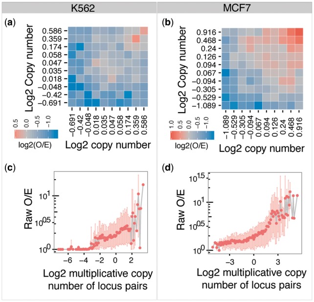
DNA copy number is positively correlated with Hi-C contact counts in K562 and MCF7 cells. (a, b) The 2D bias plot demonstrates that log2 copy number ratios are positively correlated with contact counts in 1 Mb resolution Hi-C maps. Genomic bins of different log2 copy number ratios are subdivided into 10 quantile groups. All bin pairs are mapped into the 10 × 10 quantile group pairs. Each tile in the plot is the median log2 ratio of observed over expected (O/E) in each quantile group pair. Red represents situations in which more reads than expected were detected; blue means fewer reads than expected were detected; grey means equal reads than expected were detected; white means no locus pair with Hi-C reads was mapped in the quantile group pair. (c, d) Positive correlation between raw O/E ratios and log2 multiplicative copy number in 1 Mb resolution Hi-C maps. The log2 multiplicative copy number was calculated by adding the log2 ratios of copy numbers of the two genomic bins of each locus pair. The log2 multiplicative copy number was converted to discrete numbers by rounding to one decimal. Dark colored dots are the mean O/E values; light colored areas are the 95% CIs of the data

3.2 Chromosome-adjusted iterative correction

The iterative correction (IC) method based on the matrix balancing algorithm is one of the most widely used methodologies to remove both explicit and unknown biases from Hi-C data (Ay and Noble, 2015). The advantage of the IC method is that it provides an ICB vector, instead of a bias matrix, which contains all information used to correct the Hi-C data matrix. The IC method (also called ICB correction) has been demonstrated to work well in normal samples and cell lines (Ay and Noble, 2015; Imakaev et al., 2012; Li et al., 2015; Rao et al., 2014; Sauria et al., 2015), which have uniform copy number genomes. However, the ICB correction should not be directly applied to data from tumor samples, such as the K562 cell line, because such samples display a significant degree of variation in copy number across chromosomes (Supplementary Fig. S5). The ICB correction is preferentially applied chromosome by chromosome to prevent overloading computational resources when analyzing high-resolution Hi-C maps (Ay and Noble, 2015; Sauria et al., 2015). Use of the ICB correction leads to an uncorrected chromosome-level bias (cbias) (Figs 2 and 3a–d), thus causing biased calling results of significant contacts (Fig. 3e). This bias cannot simply be adjusted for by using total or average contact counts of chromosomes due to the length differences of chromosomes (Supplementary Fig. S6). In Hi-C data, contact counts decrease with increasing genomic distances such that smaller chromosomes have fewer long distance locus pairs than larger chromosomes. This observation leads to the fact that average contact counts of chromosomes are negatively correlated with chromosome length (Supplementary Fig. S6a), and total contact counts of chromosomes are positively correlated with chromosome length (Supplementary Fig. S6b). For the K562 cell line, the chromosome bias is very apparent, especially for chromosome 9 in lower resolution Hi-C maps (Fig. 3a and Supplementary Fig. S5). Further analysis shows that chromosome-level copy numbers are highly correlated with chromosome-level Hi-C contact O/E ratios even after ICB correction (Fig. 3b).

Fig. 2.

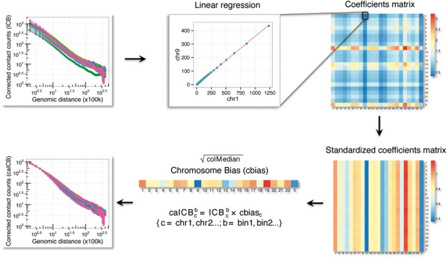
An overview of the caICB correction algorithm. The algorithm first calculates the empirical mean of contact counts over genomic distances for all chromosomes in any resolution of an ICB-corrected contact matrix. We used linear regression, forcing the intercept to be 0 in each chromosome pair, to generate a coefficient matrix. The coefficient matrix is further standardized and summarized as a cbias which is then used to adjust the original ICB to obtain the caICB-corrected Hi-C map with minimal differences among chromosomes

Fig. 3.

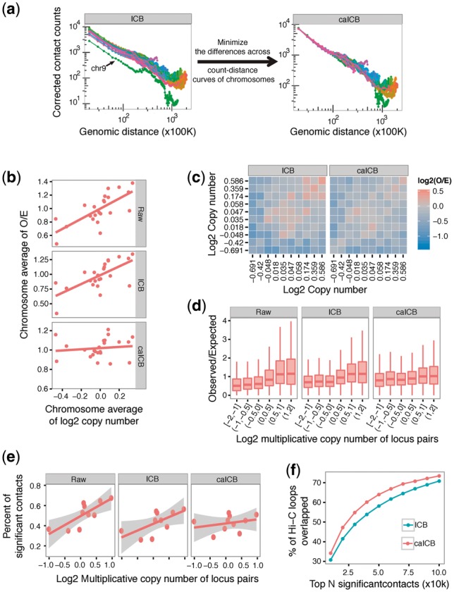
Performance of the caICB correction compared with raw data and ICB correction using the 1 Mb K562 Hi-C map as an example. (a) Schematic of the caICB algorithm, which minimizes the differences across count-distance curves of different chromosomes. The count-distance curve is plotted: Hi-C read pairs are binned into 1 Mb resolution bins. Bin level counts data are normalized by the ICB (left) and caICB (right), respectively. Mean corrected contact counts among all bin pairs for each genomic distance are shown as dots, and dots representing data from the same chromosome are connected by lines. Each chromosome is displayed in a different color. (b) The relationship between chromosome-level observed divided by expected counts (O/E) and chromosome-level copy number. The mean O/E among all locus pairs for each chromosome is calculated as chromosome-level O/E. The mean copy number among all locus pairs for each chromosome is determined as chromosome-level copy number. Linear regression fits are shown as lines. Note that the chromosome-level copy number bias is largely corrected by the caICB methodology. Raw: raw Hi-C data; ICB: ICB-corrected Hi-C data. caICB: caICB-corrected Hi-C data. (c) The 2D bias plot of ICB- and caICB-corrected Hi-C maps. The raw Hi-C map is shown in Figure 1a. (d) Locus pairs are binned into six bins based on log2 multiplicative copy number. O/E ratios of all locus pairs in each bin are shown in the boxplots. O/E distributions of all locus pairs in different log2 multiplicative copy number bins are significantly improved after caICB correction. (e) Significant contact calls. Calls for significant contacts are biased to high copy number genomic loci, and can be corrected for by the caICB correction. In the analyses, we use Fit-Hi-C to identify significant contacts using the raw data, ICB- and caICB-corrected matrices, respectively. Contacts with q-value < 0.01 are identified as significant. All contacts of different log2 multiplicative copy number are divided into 10 quantile groups. Within each quantile group, the percent of significant contacts to all contacts is calculated and shown as dots. The linear regressions as well as 95% CI are displayed. (f) Overlap between Hi-C loops identified by HiCCUPs and significant contacts identified from ICB- and caICB-corrected results. The top N significant contacts identified by Fit-Hi-C using both ICB- and caICB-corrected Hi-C matrices overlap with Hi-C loops, with a larger number of overlaps found for the caICB as compared with the ICB method

To correct for this particular source of bias, we designed a linear regression-based chromosome-level adjustment method called caICB (Fig. 2), which represents an extension of ICB correction. We performed our analyses on multiple resolution contact maps (1 Mb, 250, 100 and 10 Kb) in K562. The algorithm initiates with the ICB corrected Hi-C data matrix. Our method assumes equal representation of genomic locus pairs with similar genomic distances located on different chromosomes if there were no bias in the Hi-C maps. Our approach first calculates the empirical mean of contact counts over genomic distances for all chromosomes. We used linear regression by forcing the intercept to be 0 in each chromosome pair to generate a coefficient matrix. The coefficient matrix is further standardized and summarized as a cbias vector. This vector is then used to adjust the original ICB- to obtain the caICB-corrected data (Fig. 2). The caICB correction minimizes the difference among chromosomes (Fig. 3a) and organically corrects for chromosome-level copy number biases (Fig. 3a and b, Supplementary Figs S7 and S8). The caICB corrected O/E ratio provides an unbiased Hi-C map for different copy number regions across different resolutions (Fig. 3c and d and Supplementary Fig. S9).

3.3 The caICB correction leads to unbiased significant contact calling results

Most Hi-C analyses report a list of significant contacts (Dixon et al., 2012, 2015; Jin et al., 2013; Rao et al., 2014), no matter whether the study was designed to ultimately investigate folding principles of the genome (Rao et al., 2014) or long-range DNA interactions (Jin et al., 2013). Therefore, an unbiased significant contact list is an essential starting point for the downstream functional analysis or modeling of Hi-C data. Here we applied Fit-Hi-C (Ay et al., 2014), which uses a spline fitting followed by a binomial test to investigate whether there were significantly more contact counts than expected in the same genomic distances, to identify significant contacts in potentially interesting genomic regions of four resolution Hi-C maps of K562 cells. By selecting a q-value < 0.01 as the significance threshold, we found that significant contacts are biased to high copy number genomic loci for un-corrected Hi-C maps of a non-uniform copy number genome, such as that of tumor cells (Fig. 3e). This finding demonstrates that a correction is necessary for Hi-C data of tumor samples and other cell types with copy number variation. The caICB correction leads to a nearly unbiased significant contact calling result, unlike the ICB correction (Fig. 3e and Supplementary Fig. S10). Taking the 100 Kb resolution map as an example, the standard deviation of the percent of significant contacts across all copy number groups for caICB correction results is 0.017, which is only half (0.035) that of ICB correction results and one-fourth (0.071) that of un-corrected results. The regression curves of 1 Mb resolutions are much flatter for caICB-corrected results (regression slope = 0. 04, P = 0.44) than for ICB-corrected (regression slope = 0.13, P = 0.04) and raw results (regression slope = 0.18, P = 0.007) (Fig. 3e), which indicates a more efficient bias elimination by the caICB as compared with the ICB correction. Similar results were also observed in other resolutions (Supplementary Fig. S10). In addition, when choosing the top N significant contacts identified from both the ICB- and caICB-corrected matrices and comparing them with Hi-C loops identified by HiCCUPs for K562 cells (Rao et al., 2014), we found that the caICB correction provides higher overlapping results with Hi-C loops than the ICB correction (Fig. 3f).

3.4 Performance of caICB for all known explicit bias factors

In previous studies (Hu et al., 2012; Yaffe and Tanay, 2011), 2D bias plots were used as an evaluation measurement of the normalization step. We therefore utilized a similar approach to investigate the performance of the caICB correction with regard to known explicit biases. We first confirmed that, by comparing to raw O/E values as well as residual scores across different methods (Fig. 4 and Supplementary Fig. S11), the ICB correction significantly reduces all three explicit biases—mappability, GC bias and fragment length—at different resolutions. As expected, the caICB correction performs similarly well with respect to these biases. For instance, the reduction in the fragment length bias is similar between the ICB and caICB corrections (Fig. 4a). The GC content bias is also largely unchanged between ICB and caICB corrections, except for a slight increase in the 100 Kb resolution map in caICB; however, the overall distribution of all tile residuals is unchanged (Supplementary Fig. S11b). Furthermore, mappability is a bias factor that may benefit from the caICB correction; consistent with this expectation, we observed a clear decrease of both mean and variance of the distribution of tile residuals for mappability in lower resolution maps (weighted t-test P = 2.1E-4 for 1 Mb and P = 5.3E-4 for 250 Kb), but not in higher resolution maps (Fig. 4 and Supplementary Fig. S11). Most importantly, the caICB correction significantly reduces the copy number bias in lower resolution maps (weighted t-test P = 1.6E-4 for 1 Mb and P = 0.03 for 250 Kb, Fig. 4 and Supplementary Fig. S11). For the highest resolution investigated, the 10 kb map, the decrease of the mean residual score is not as significant as that in lower resolution maps after caICB correction, but the variance of the residuals is significantly decreased (Supplementary Figs S11c and S12). Similar results were also observed for the 100 Kb map (Supplementary Figs S11b and S12). Therefore, we found that the caICB correction significantly reduces the copy number bias in all resolution maps without increasing the other sources of bias, and can furthermore potentially reduce some of the biases such as mappability in certain resolutions.

Fig. 4.

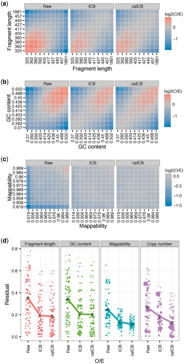
Effects of the ICB and caICB corrections on four know explicit bias factors in 1 Mb K562 Hi-C maps. Fragment length (a), GC content (b), and mappability (c) are shown in 2D bias plots. Genomic bins of 1 Mb are cut into 10 quantile groups. All bin pairs are mapped into the 10 × 10 quantile group pairs. Each tile in the plot is the median log2 ratio of O/E in each quantile group pair. Red represents situations in which more reads than expected were detected; blue means fewer reads than expected were detected; grey means equal reads than expected were detected d. (e) Residual plots show a quantitative evaluation of the performance of different correction algorithms on four bias factors. The residual is calculated by subtracting one from the value in each tile; a residual of all zero provides an unbiased Hi-C map. Residuals of tiles in a-d are plotted as dots, and the dot size represents the number of locus pairs in each tile. The mean values of residuals weighted by dot sizes are calculated within each group and are shown as black dots

3.5 Stabilization of the caICB correction

The main goal of the caICB correction algorithm is to capture and correct for the cbias in Hi-C maps. The cbias results obtained for different resolutions of Hi-C maps of the K562 cell line are overall similar, but there are minor differences. For instance, the cbias vector of chr9 in lower resolution Hi-C maps is around 0.6 but is 0.75 in the 10 Kb Hi-C map. In another case, the cbias vector of chr4 is decreased with the resolution increase (Fig. 5a). Therefore, the cbias results cannot be shared across all resolution Hi-C maps, and need to be calculated separately for different resolution Hi-C maps. To calculate the cbias in extremely high-resolution Hi-C maps (≤10 Kb), it is preferable to choose a small genomic range to perform the algorithm instead of using the whole contact map, since this approach significantly increases the running speed and reduces memory usage. In the methodology, the parameter K represents the tuning parameter for choosing the nearest K binning steps of each genomic locus to perform the algorithm (see Section 2). We tested the algorithm by using different values of K for 100 Kb Hi-C maps, and found that the resulting cbias vectors were very stable across different values of K from 5 to 800 (Fig. 5b). Especially when K is larger than 100, the cbias vectors were identical across different values of K, up to two decimal places (Fig. 5b). Therefore we concluded that the algorithm is robust with regard to using a subset of genomic ranges, and we used K = 200 in this study. In general, we recommend using a K such that K times the resolution is equal to the genomic range that users are interested in.

Fig. 5.

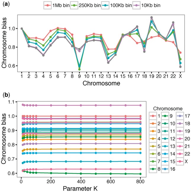
Stabilization of the caICB correction. (a) cbias varies across different resolution HiC maps. cbias is calculated for 1 Mb, 250, 100 and 10 Kb resolution K562 Hi-C maps, respectively. (b) cbias is stable with different values of the parameter K measured in the 100 Kb Hi-C map. Different colors represent different chromosomes

3.6 Application to other datasets

In addition to K562 cells, we also applied the caICB correction to MCF7 Hi-C data, which has a higher level of copy number variation (Supplementary Fig. S13). The 2D bias plots show that the caICB correction can successfully eliminate the copy number bias (Supplementary Fig. S14a and b). We furthermore surveyed chromosome-level copy number differences in all CCLE tumor cell lines (Barretina et al., 2012) and found that a substantial number of tumor cell lines (∼75% of all CCLE tumor cell lines) display an even higher level of chromosome-level copy number variations than K562 cells (Supplementary Fig. S14c). This finding demonstrates that chromosome-level copy number bias is very common in tumor Hi-C data, which makes the caICB correction a widely applicable normalization algorithm for studying the 3D genome of cancer cells.

4 Conclusion

Our proposed method, caICB, is able to efficiently correct for the copy number bias as well as other potential biases in tumor Hi-C data without a priori knowledge of these biases. Our method is suitable for extremely high-resolution Hi-C maps, because it can achieve robust results when using a small subset of genomic ranges instead of using the whole genome contact map. The method does not require copy number data for the samples for which Hi-C data are available, and has the potential to adjust for other possible biases in Hi-C data without their priori knowledge. Despite the fact that copy number data is not required for the caICB correction algorithm, it would be preferable to monitor copy number bias in the data before and after normalization when analyzing Hi-C data in tumor samples. This observation arises because for extreme cases, such as high-level amplification or near homozygous deletion, which accounts for <1% of all locus pairs in K562 cells but may account for a larger fraction in other tumor cells, the contact counts might either be too high or too low to be corrected for by current methods. In these cases, careful evaluation of normalization results is necessary to prevent making biased conclusions.

Notably, we found that within-chromosome copy number biases are very effectively corrected by the original ICB method. Therefore, downstream analyses, such as Hi-C loops identified by HiCCUPs, are not biased even when using ICB-corrected Hi-C maps, because the background model is built locally within each chromosome. However, downstream analyses using the genome-wide background, such as the identification of significant contacts by Fit-Hi-C, can be significantly biased in ICB-corrected Hi-C maps; this bias is largely eliminated by using the proposed caICB correction. Furthermore, the caICB correction makes the Hi-C contact counts comparable across the genome, and has potential application for comparing Hi-C data between tumor and normal cells with different genomic copy numbers.

Funding

Dana-Farber Cancer Institute Physical Sciences-Oncology Center; grant number: NIH U54CA193461.

Conflict of Interest: none declared.

References

- Ay F. et al. (2014) Statistical confidence estimation for Hi-C data reveals regulatory chromatin contacts. Genome Res., 24, 999–1011. [DOI] [PMC free article] [PubMed] [Google Scholar]
- Ay F., Noble W.S. (2015) Analysis methods for studying the 3D architecture of the genome. Genome Biol., 16, 183.. [DOI] [PMC free article] [PubMed] [Google Scholar]
- Barretina J. et al. (2012) The Cancer Cell Line Encyclopedia enables predictive modelling of anticancer drug sensitivity. Nature, 483, 603–607. [DOI] [PMC free article] [PubMed] [Google Scholar]
- Barutcu A.R. et al. (2015) Chromatin interaction analysis reveals changes in small chromosome and telomere clustering between epithelial and breast cancer cells. Genome Biol., 16, 214. [DOI] [PMC free article] [PubMed] [Google Scholar]
- De S., Michor F. (2011) DNA replication timing and long-range DNA interactions predict mutational landscapes of cancer genomes. Nat. Biotechnol., 29, 1103–1108. [DOI] [PMC free article] [PubMed] [Google Scholar]
- Derrien T. et al. (2012) Fast computation and applications of genome mappability. PloS One, 7, e30377. [DOI] [PMC free article] [PubMed] [Google Scholar]
- Dixon J.R. et al. (2015) Chromatin architecture reorganization during stem cell differentiation. Nature, 518, 331–336. [DOI] [PMC free article] [PubMed] [Google Scholar]
- Dixon J.R. et al. (2012) Topological domains in mammalian genomes identified by analysis of chromatin interactions. Nature, 485, 376–380. [DOI] [PMC free article] [PubMed] [Google Scholar]
- Fudenberg G. et al. (2011) High order chromatin architecture shapes the landscape of chromosomal alterations in cancer. Nat. Biotechnol., 29, 1109–1113. [DOI] [PMC free article] [PubMed] [Google Scholar]
- Fullwood M.J. et al. (2010) Chromatin interaction analysis using paired-end tag sequencing. current protocols in molecular biology In: Ausubel F. M., Brent R., Kingston R. E., Moore D. D., Seidman J. G., Smith J. A., Struhl K. (eds.) Current Protocols in Molecular Biology, John Wiley and Sons, New York;Chapter 21:Unit 21 15 21–25. [DOI] [PMC free article] [PubMed] [Google Scholar]
- Hanahan D., Weinberg R.A. (2011) Hallmarks of cancer: the next generation. Cell, 144, 646–674. [DOI] [PubMed] [Google Scholar]
- Hu M. et al. (2012) HiCNorm: removing biases in Hi-C data via Poisson regression. Bioinformatics, 28, 3131–3133. [DOI] [PMC free article] [PubMed] [Google Scholar]
- Huang J. et al. (2015) Predicting chromatin organization using histone marks. Genome Biol., 16, 162. [DOI] [PMC free article] [PubMed] [Google Scholar]
- Imakaev M. et al. (2012) Iterative correction of Hi-C data reveals hallmarks of chromosome organization. Nat. Methods, 9, 999–1003. [DOI] [PMC free article] [PubMed] [Google Scholar]
- Jin F. et al. (2013) A high-resolution map of the three-dimensional chromatin interactome in human cells. Nature, 503, 290–294. [DOI] [PMC free article] [PubMed] [Google Scholar]
- Kalhor R. et al. (2012) Genome architectures revealed by tethered chromosome conformation capture and population-based modeling. Nat. Biotechnol., 30, 90–98. [DOI] [PMC free article] [PubMed] [Google Scholar]
- Knight P., Ruiz D. (2013) A fast algorithm for matrix balancing. IMA J. Numer. Anal., 33, 1029–1047. [Google Scholar]
- Le T.B. et al. (2013) High-resolution mapping of the spatial organization of a bacterial chromosome. Science, 342, 731–734. [DOI] [PMC free article] [PubMed] [Google Scholar]
- Li W. et al. (2015) Hi-Corrector: a fast, scalable and memory-efficient package for normalizing large-scale Hi-C data. Bioinformatics, 31, 960–962. [DOI] [PMC free article] [PubMed] [Google Scholar]
- Lieberman-Aiden E. et al. (2009) Comprehensive mapping of long-range interactions reveals folding principles of the human genome. Science, 326, 289–293. [DOI] [PMC free article] [PubMed] [Google Scholar]
- Liu L. et al. (2013) DNA replication timing and higher-order nuclear organization determine single-nucleotide substitution patterns in cancer genomes. Nat. Commun., 4, 1502.. [DOI] [PMC free article] [PubMed] [Google Scholar]
- Nagano T. et al. (2013) Single-cell Hi-C reveals cell-to-cell variability in chromosome structure. Nature, 502, 59–64. [DOI] [PMC free article] [PubMed] [Google Scholar]
- Naumova N. et al. (2013) Organization of the mitotic chromosome. Science, 342, 948–953. [DOI] [PMC free article] [PubMed] [Google Scholar]
- Pope B.D. et al. (2014) Topologically associating domains are stable units of replication-timing regulation. Nature, 515, 402–405. [DOI] [PMC free article] [PubMed] [Google Scholar]
- Quinlan A.R., Hall I.M. (2010) BEDTools: a flexible suite of utilities for comparing genomic features. Bioinformatics, 26, 841–842. [DOI] [PMC free article] [PubMed] [Google Scholar]
- Rao S.S. et al. (2014) A 3D map of the human genome at kilobase resolution reveals principles of chromatin looping. Cell, 159, 1665–1680. [DOI] [PMC free article] [PubMed] [Google Scholar]
- Rickman D.S. et al. (2012) Oncogene-mediated alterations in chromatin conformation. Proc. Natl. Acad. Sci. USA, 109, 9083–9088. [DOI] [PMC free article] [PubMed] [Google Scholar]
- Sauria M.E. et al. (2015) HiFive: a tool suite for easy and efficient HiC and 5C data analysis. Genome Biology, 16, 237. [DOI] [PMC free article] [PubMed] [Google Scholar]
- Servant N. et al. (2012) HiTC: exploration of high-throughput 'C' experiments. Bioinformatics, 28, 2843–2844. [DOI] [PMC free article] [PubMed] [Google Scholar]
- Seshan V., Olshen A. (2016) DNAcopy: DNA copy number data analysis. R package version 1.44.0.
- Shavit Y., Lio P. (2014) Combining a wavelet change point and the Bayes factor for analysing chromosomal interaction data. Mol. bioSyst., 10, 1576–1585. [DOI] [PubMed] [Google Scholar]
- Sinkhorn R., Knopp P. (1967) Concerning nonnegative matrices and doubly stochastic matrices. Pacific J. Math., 21, 343–348. [Google Scholar]
- Wingett S. et al. (2015) HiCUP: pipeline for mapping and processing Hi-C data. F1000Research, 4, 1310. [DOI] [PMC free article] [PubMed] [Google Scholar]
- Yaffe E., Tanay A. (2011) Probabilistic modeling of Hi-C contact maps eliminates systematic biases to characterize global chromosomal architecture. Nat. Genet., 43, 1059–1065. [DOI] [PubMed] [Google Scholar]
Associated Data
This section collects any data citations, data availability statements, or supplementary materials included in this article.