Abstract
PURPOSE
The bias and variance of high angular resolution diffusion imaging (HARDI) methods have not been thoroughly explored in the literature and may benefit from the simulation extrapolation (SIMEX) and bootstrap techniques to estimate bias and variance of HARDI metrics.
METHODS
The SIMEX approach is well established in the statistics literature and uses simulation of increasingly noisy data to extrapolate back to a hypothetical case with no noise. The bias of calculated metrics can then be computed by subtracting the SIMEX estimate from the original pointwise measurement. SIMEX has been studied in the context of diffusion imaging to accurately capture the bias in fractional anisotropy (FA) measurements in diffusion tensor imaging (DTI). Herein, we extend the application of SIMEX and bootstrap approaches to characterize bias and variance in metrics obtained from a Q-ball imaging (QBI) reconstruction of HARDI data.
RESULTS
The results demonstrate that SIMEX and bootstrap approaches provide consistent estimates of the bias and variance of generalized fractional anisotropy (GFA), respectively. The root mean squared error (RMSE) for the GFA estimates shows a 7% decrease in white matter and an 8% decrease in gray matter when compared to the observed GFA estimates. On average, the bootstrap technique results in standard deviation estimates that are about 97% of the true variation in white matter, and 86% in gray matter.
CONCLUSION
Both SIMEX and bootstrap methods are flexible, estimate population characteristics based on single scans, and may be extended for bias and variance estimation on a variety of HARDI metrics.
Keywords: HARDI, Q-ball, bias correction, SIMEX, bootstrap, GFA
INTRODUCTION
Diffusion-weighted magnetic resonance imaging (DW-MRI) is an image acquisition technique that utilizes the natural diffusion of water within the human body to non-invasively study tissue microstructure. High angular resolution diffusion imaging (HARDI) is able to identify crossing fiber orientations, while diffusion tensor imaging (DTI) is unable to discern fibers in more than a single direction.
The accuracy, precision, and sensitivity of DTI have been studied and noise has been shown to have an impact on the bias and variance of DTI-derived metrics, such as FA (1–10). Previous work has applied the statistical concept of simulation extrapolation (SIMEX) (11,12) in an effort to quantify the bias in an observed data acquisition (1,2). This work extends the application of SIMEX to a single, empirical HARDI acquisition fit with a Q-ball model.
Bias and variance play a critical role in any statistical analysis. The appropriate balance between bias and variance allows for optimal information gain. It is not enough to have an unbiased estimator (i.e., an estimator that estimates the correct quantity, on average) if the variance is comparatively large (i.e., the estimate is imprecise). Similarly, an estimate with very small variance but large bias is very precise, but will not converge to the correct value as the sample size increases. Each situation can be useful, depending on the goals of the study, but a balance between the two is considered optimal. Thus, it is important to evaluate the methods that we use in terms of the bias and variance of the estimates we produce. The ability to quantify the bias and variance between different imaging and analysis methods quickly and easily allows the researcher to make informed design decisions at every step. Currently, there are no methods available for bias correction in HARDI acquisitions. This paper provides approaches for the quantification of both bias and variance that can be performed with a single data acquisition, allowing for the comparison across methods without requiring repeated data acquisitions.
In addition to the simple quantification of bias for better understanding of the quality of a variety of imaging acquisition parameters and model fitting strategies, this method may also prove useful as a tool for bias correction. Several acquisition parameters are set during the image acquisition process, all of which can affect scan quality and the resulting analysis. Of particular interest is the situation where two scans are taken at different acquisition settings on the same subject. In theory, scans should be comparable within subjects, but in practice, they can be extremely variable. The SIMEX process aims to provide a method for bias-correction while the bootstrap procedure allows for an empirical estimate of the variance of Q-ball metrics, such as generalized fractional anisotropy (GFA), which is a measure of anisotropy calculated from the orientation distribution function (ODF).
THEORY
This analysis focuses on Q-ball imaging reconstruction of the ODF of HARDI data acquisitions. We evaluate methods detailed by (13) and (14) that use a spherical harmonic basis in the reconstruction of the ODF, which describes the patterns of diffusion within the tissue.
The regularized Q-ball reconstruction introduced in (14) requires the m × 1 vector of diffusion weighted signals at each voxel, as well as a 2 × m matrix of gradient directions in spherical coordinate space, where m is the number of gradient directions. Details on the calculation of the ODF are found in (14).
Following calculation of the ODF, a variety of metrics can be calculated. The metric used in this analysis is GFA, which is given by,
where ψ is the ODF vector, and ψ̅ is its mean (15).
SIMEX applied to empirical data
The SIMEX approach detailed herein estimates the bias present in metrics generated by a Q-ball model. SIMEX was introduced as a method for performing inference in models where measurement error was a concern. This method is unique in that it does not require fitting a complicated parametric measurement error model, yet still provides unbiased estimates of the object of interest. In short, bias estimates can be calculated by adding increasing amounts of synthetic noise to the data and computing the desired metrics at each noise level. The resulting measures can be extrapolated to the hypothetical case where no noise is present (12).
In the case where the measurement error variance can be well estimated, SIMEX is able to estimate the bias without requiring any model fitting, as is generally the case in typical measurement error estimation and correction procedures. SIMEX requires that the measurement error variance is well estimated and that the metric of interest changes monotonically as a function of noise added.
In this section, we adopt the notation established by Lauzon et al. in (1). We assume Xtruth to be a truth dataset with zero noise. This dataset can be used to calculate the ground truth metric, GFAtruth, via a Q-ball fit. Now, assume an observed dataset with experimental noise where σE represents the standard deviation of the noise at each voxel. This observed dataset is given by,
which represents the addition of stacked Rician noise with standard deviation σE as in (2). While the original SIMEX approach assumes a normally distributed noise term, we are able to substitute the Rician distribution due to its approximation of a Gaussian distribution at SNR greater than 3 (16). The metrics resulting from a Q-ball fit of this observed data are given by GFAobs.
The “simulation” portion of the SIMEX procedure begins with the simulation of noisy GFA observations. These noisy observations cannot be simulated directly, thus a series of Monte Carlo simulations are performed via the addition of stacked Rician noise with the standard deviation of ω1/2σE, given by,
where M.C. represents a Monte Carlo replication and metrics derived from XM.C.(ω) are given by GFAM.C.(ω). The average value within each set of replications with a given ω value is given by .
Once a trend is established in the sequence of values, a quadratic equation is fit.
The variance of the simulated, noisy data can be viewed as a function of ω,
Thus, the variance goes to zero when ω = −1 and the value of GFA at this value is considered noiseless. The value at ω = −1 is referred to as GFASIMEX.
Finally, the bias can be estimated by subtracting the SIMEX metrics from those calculated from the observed data:
| (1) |
The true bias can be calculated, given truth data, by
| (2) |
Bootstrap estimation of variance
The bootstrap is a popular method for estimation of variance in models where a parametric solution is either not available or not assumed. The family of bootstrap procedures involves the resampling of data with replacement, where each resampled dataset is viewed as a surrogate for an independently sampled dataset. The metric of interest is computed for each resampled dataset. Through repeated sampling, we can create a bootstrap distribution of the metric, which approximates the true sampling distribution of the metric (17).
In a case where multiple acquisitions were obtained for each gradient direction, a classic bootstrap approach works well. In a classic bootstrap, data points are resampled across the acquisitions, but within each voxel. The requirement for repeated acquisitions, however, is unreasonable for larger numbers of gradient diffusion directions. The residual bootstrap, in which residuals are resampled at random across data points, cannot be used with a single DW-MRI acquisition due to the heteroscedasticity (i.e. non-constant variance across gradient directions) that is introduced upon permutation (18,19). While the signal used for Q-ball does not use a log-transform (as in DTI), we may still observe some heteroscedasticity as a result of differences in the variance of the Rician distribution as a function of the mean.
In cases where the errors are heteroscedastic, the wild bootstrap has proven effective at characterizing the variance without assuming constant variance (20). This method was applied to DTI in (19) and was shown to outperform the regular bootstrap for a variety of settings. The wild bootstrap has since been applied in probabilistic fiber tracking with positive results (21). For these reasons, we chose to employ the wild bootstrap for our variance estimation procedure as follows.
A wild bootstrap technique gives empirical estimates of the variance of popular metrics from a Q-ball fit. Continuing the notation established above, we begin with the truth data, Xtruth with zero experimental noise. n datasets are simulated via the addition of Rician noise with standard deviation σE. These datasets are seen as hypothetical independent acquisitions from a single subject. These datasets are fit using the Q-ball and GFA for each voxel is calculated. The standard deviation of the resulting calculations gives σtrue.
Next, variance is estimated via the wild bootstrap procedure. First, residuals must be calculated at each voxel,
| (3) |
In order to create the bootstrapped datasets, the signs of the residuals are flipped randomly and added back to the observed data (21). The signs of the residuals are determined by a vector of random Bernoulli draws of the same length as the residual vector:
| (4) |
where Xobs is the m × 1 vector of observed data at a single voxel and B is an m × 1 vector of random Bernoulli draws. This process is repeated n times, resulting in n simulated datasets. GFA is calculated for each simulated dataset and the standard deviation of GFA across the n datasets gives σ̂.
METHODS
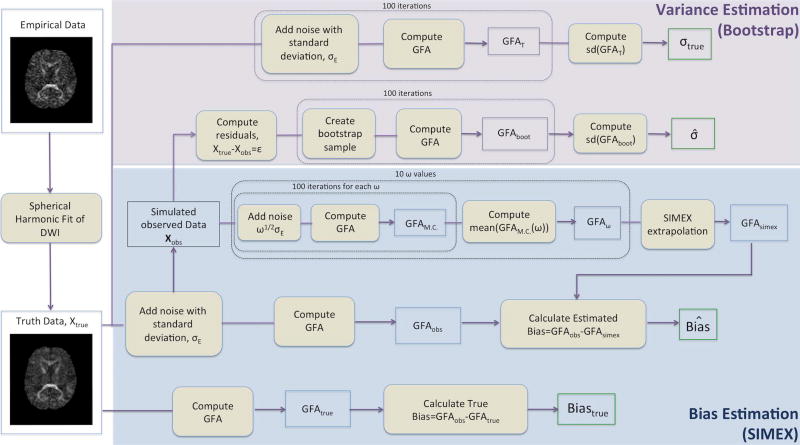
A flowchart detailing the steps of the SIMEX process on GFA as well as the calculation of bootstrap variance is given in Figure 1. The SIMEX procedure is performed on a voxel-by-voxel basis, where each voxel is evaluated independently. All calculations were performed in Matlab version R2016a (MathWorks, Natick, MA). (22) and the Camino Diffusion MRI toolkit (23).
Figure 1.
Flowchart detailing the SIMEX and bootstrap procedures. The flowchart begins with the creation of the true data via a spherical harmonic fit of the empirical data as detailed in the text. The top two sections refer to the calculation of the estimated and true standard deviation for GFA. The calculation of true standard deviation is based on the true data while the calculation of the estimated standard deviation is based on the noise-added simulated observed data. The SIMEX procedure begins with the simulated observed data, iterates through a series of noise values and concludes with the extrapolation to estimate GFA. True bias requires the calculation of GFA based on the truth data and comparison with the observed GFA as calculated from the simulated observed data.
Empirical Data
The empirical data used in this experiment were obtained from a healthy volunteer using a 3T Philips Scanner with a 32-channel head coil. The session consisted of 96 gradient directions at a b-value of 3000 s/mm2. The voxel resolution is 2.5mm × 2.5mm × 2.5mm with 38 slices. The scan parameters were: Multi-Band=2; SENSE=2.2; TR= 2650 ms; TE=94 ms; partial Fourier=0.7. Fold over direction was A-P with a P (posterior) fat shift. For each shell, an additional diffusion scan was acquired with reverse phase encoded volumes (i.e., fold over direction A-P with A fat shift) with a minimally weighted volume and 3 diffusion weighting directions with a b-value of 1000 s/mm2 along the imaging frame cardinal directions, and all other parameters were kept constant. All data were acquired in accordance with the Vanderbilt University Institutional Review Board (IRB) guidelines and with the signed consent of the volunteer.
Creating Ground Truth Data
To create the ground truth data used in this experiment, the 6th degree spherical harmonic basis function was selected. This basis function was generated using the b-vectors used in the original data acquisition. Regularized linear least squares fitting was used to estimate the spherical harmonic coefficients of the diffusion-weighted signal for each voxel. The resulting spherical harmonic series representation is a smoothed version of the original data; thus the resulting brain volume is assumed to be noiseless and is used as the ground truth dataset for the entirety of this analysis. Note that this method depends heavily on the appropriateness of the Q-ball model. Any deviation from the model may result in a systematic bias that cannot be corrected via the SIMEX procedure. Care must be taken when fitting the truth model to avoid such bias. This dataset, along with the b-values and b-vectors can be found here: www.nitrc.org/projects/masimatlab under “SIMEX on HARDI.”
Creating Observed Data
The observed data, Xobs, were created via the addition of random Rician noise to the ground truth data. The standard deviation of the Rician noise is the standard deviation of the residuals, σE, thus this observed dataset approximates an empirically observed HARDI data acquisition at the given SNR.
SIMEX
Calculating Estimated Bias The first step of the SIMEX process is to calculate . 100 Monte Carlo simulations were performed for each ω = 1, 2, …, 10, and the average was taken for each ω to obtain . A quadratic equation was fit in order to extrapolate to the GFA value that results when ω = −1. The resulting value is known as GFASIMEX. GFAobs was obtained directly from a Q-ball fit of the observed data, Xobs. Estimated bias was calculated as the difference between GFASIMEX and GFAobs (Eq. 1).
Calculating True Bias
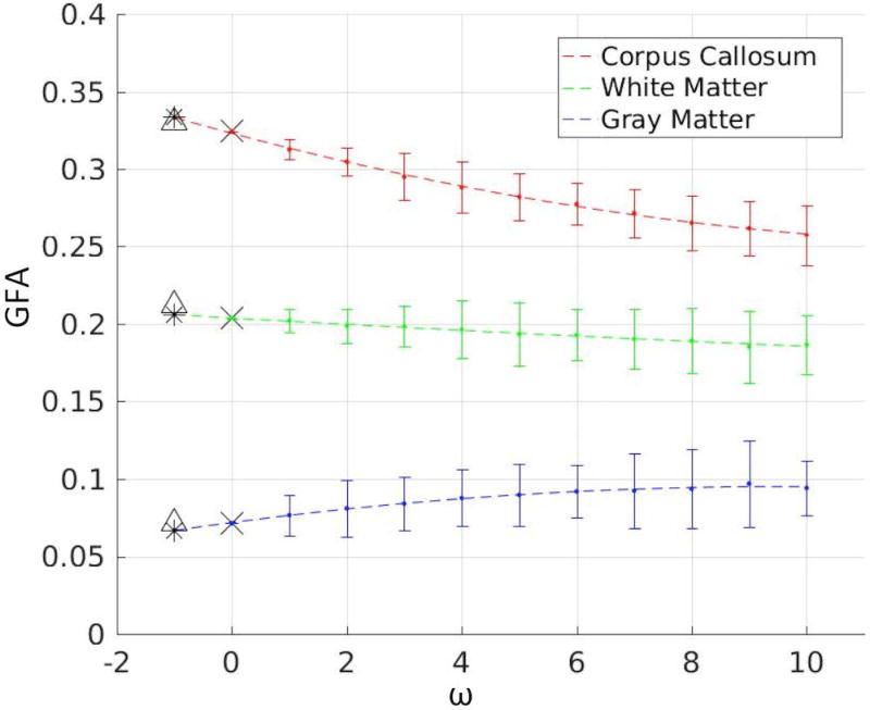
In order to calculate the true bias, the GFA of Xobs was calculated via a Q-ball fit. GFAtruth was calculated by Xtruth with no additional noise. True bias was calculated by taking the difference between GFAobs and GFAtruth (Eq. 2). An example of the SIMEX procedure on 3 voxels from different brain regions is shown in Figure 2. A successful SIMEX procedure is one where the SIMEX estimated GFA value is closer to the true GFA value than the observed GFA value, i.e., the estimated bias is close to the true bias.
Figure 2.
The SIMEX procedure demonstrated on 3 distinct voxels within the brain. These three voxels show the three possible results of the SIMEX procedure: when the SIMEX estimate improves the observed estimate, when the SIMEX estimate is approximately equal to the observed estimate, and when the SIMEX estimate is worse than the observed estimate. ω is the multiplier on the amount of noise added to each voxel (note that ω=0 is the observed data and ω=−1 is the noiseless true data). The dashed lines represent the SIMEX quadratic fit and extrapolation back to the case with zero noise (ω= −1). Each ‘•’ indicates the mean of the 100 Monte Carlo iterations at that ω value. The ‘×’ indicates the observed GFA value for that voxel. The triangles indicate the true GFA value for each voxel. The asterisks indicate the SIMEX estimated GFA value for each voxel. The error bars represent the 5th and 95th percentiles of the M.C. iterations for each ω.
This procedure was performed independently for each voxel in the brain volume.
Bootstrap
Obtaining Residuals
To obtain the necessary residuals for the residual wild bootstrap, we calculate the difference in signal between the ground truth data and the observed data (Eq. 3).
Calculating Estimated Variance
We obtain an estimate of the bootstrap variance for GFA. Residual wild bootstrap is performed using Xboot and ε (Eq. 4). We obtain 100 GFA estimates by repeating the bootstrap procedure and calculating GFA for each residual bootstrap sample. The standard deviation of the 100 metrics is taken to obtain the estimated standard deviation of the procedure, σ̂.
Calculating True Variance
Starting with the true data, Xtruth, we add random Rician noise with standard deviation, σE, to obtain an observed dataset, Xobs. The Q-ball model is fit and GFAobs is obtained. This process is repeated 100 times, resulting in 100 GFA values. The standard deviation of the 100 GFA values is considered to be the true standard deviation of the procedure, σtrue.
Characterization on Independent Datasets
We have applied the methods described above on two additional datasets to evaluate the generalizability of the approach. The second dataset is from the 2017 ISMRM TraCED challenge (https://my.vanderbilt.edu/ismrmtraced2017/). These data were acquired on a 3T Philips scanner and consisted of 64 gradient directions at a b-value of 3000 s/mm2 with a voxel resolution of 2.5mm × 2.5mm × 2.5mm with 44 slices. The scan parameters were: Multi-Band=2; SENSE=2.2; TE=99 ms; partial Fourier=0.755. Fold over direction was A-P with a P (posterior) fat shift.
The third dataset we used is from the 2015 ISMRM Tractography challenge (24). These data were obtained from an artificial phantom that was generated using the Fiberfox software. The anatomy was based on bundles segmented from a Human Connectome Project subject. These data are a 2mm isotropic diffusion acquisition with 32 gradient directions at a b-value of 1000 s/mm2. An artifact-free ground truth dataset was also provided and was used as the truth dataset in this analysis.
These two additional datasets were analyzed in the same fashion as the first, as detailed in the Methods section, with one exception for the 2015 ISMRM Tractography challenge data. Since the 2015 ISMRM Tractography challenge included a truth dataset, we opted to use it rather than the Q-ball fitted model as Xtruth.
RESULTS
Simulation Results
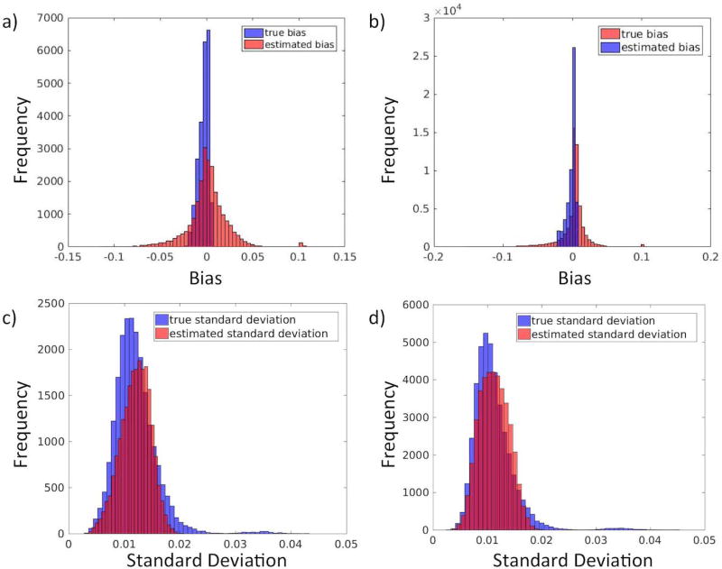
Figure 3 displays the results of the SIMEX and bootstrap procedures and their ability to estimate the true bias and standard deviation of the empirical data. Performance was evaluated on white matter and gray matter separately. The SIMEX procedure tends to underestimate the true bias of GFA in cases where the true bias is larger. The bootstrap procedure is successful at estimating the true standard deviation of GFA in both white matter and gray matter.
Figure 3.
SIMEX and bootstrap approximations of the bias and variance of GFA. a) True bias (blue) and estimated bias (red) in white matter. b) True bias and estimated bias in gray matter. c) True standard deviation and estimated standard deviation in white matter. d) True standard deviation and estimated standard deviation in gray matter. The SIMEX procedure appears to overestimate the true bias in white matter and underestimate the true bias in gray matter. The bootstrap procedure well characterizes the variance.
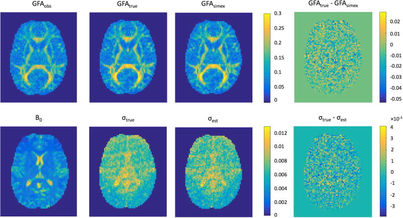
Figure 4 provides a qualitative look at the performance of SIMEX and the wild bootstrap on GFA. In this figure, we compare the true GFA values with their estimated values and compute the difference between the two, or the residual bias of our methods. Also included for reference are maps of the observed GFA and a B0 image as a structural reference. In both cases, the procedures appear to estimate their targets well. These qualitative results are in line with the quantitative results shown in Figure 3.
Figure 4.
Qualitative results demonstrate the performance of SIMEX bias-correction as well as the wild bootstrap standard deviation estimation on GFA measures at an SNR of 20:1. The approaches described here can closely estimate the true bias and standard deviation from single acquisition data with no repeated volumes. In both cases, the magnitude of the difference between the estimated and true values is several times smaller than that of the original measures (note the scales of the color bars for the difference images), thus we are able to accurately estimate both the bias and variance with these techniques. The B0 image is provided as a structural reference for the variance estimation results.
Sensitivity to noise
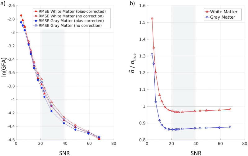
We have also provided the error of the SIMEX procedure as a function of SNR in Figure 5a. The root mean squared error (RMSE) decreases as the SNR increases for both white matter and gray matter. We have identified a typical clinical SNR range between 20:1 and 40:1 and find that the SIMEX method works well within this range.
Figure 5.
Performance of SIMEX and bootstrap across a range of SNR. (a) The root mean squared error (RMSE) of the SIMEX GFA estimation (log-scale) after bias-correction shows improvement over the RMSE without bias-correction. Within the meaningful SNR range (shown in the gray box), the bias-corrected estimates show a 5–7% improvement over the uncorrected estimates in white matter and a 5–8% improvement over the uncorrected estimates in gray matter. Within the range, lower SNR shows greater improvements. (b) The ratios of mean estimated standard deviation of GFA and mean true standard deviation of GFA within white matter and gray matter are shown across a range of SNR values. We find that the wild bootstrap procedure slightly underestimates the standard deviation in white matter, where the estimates are about 97% of the true values in our specified meaningful SNR range. In gray matter, the underestimation is larger, though the bootstrap procedure still captures 86% of the true variation. Within the typical clinical SNR range, the methods estimate the standard deviation well. Below this range, we see lower performance and above this range, we see small improvements.
The SIMEX procedure (Figure 5a) shows a 5–7% improvement over the uncorrected estimates of GFA in white matter and a 5–8% improvement over the uncorrected estimates of GFA in gray matter, within the SNR range. At lower SNR, the bias-correction procedure shows minimal improvement due to the noisy nature of the data. The largest improvements are seen in the meaningful range, though the procedure continues to result in lower RMSE at SNR up to 70:1.
To evaluate the performance of the bootstrap variance estimation procedure as a function of SNR, we examined the ratio of the estimated standard deviation and the true standard deviation for white matter and gray matter (Figure 5b). We find that within the SNR range, the wild bootstrap procedure is able to capture 97% of the true standard deviation for white matter and 86% for gray matter.
Performance on Independent Datasets
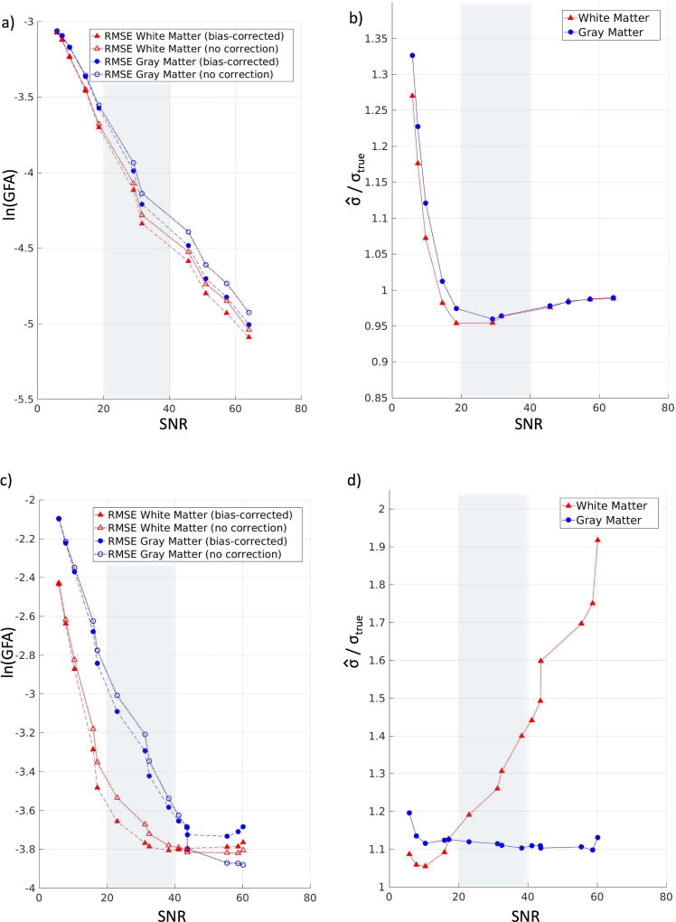
For the 2017 ISMRM TraCED challenge dataset, the SIMEX procedure (Figure 6a) shows 5–6% improvement over the uncorrected estimates of GFA in white matter and a 5–7% improvement over the uncorrected estimates of GFA in gray matter, within the SNR range. We also find that within the SNR range, the wild bootstrap procedure is able to capture about 95% of the true standard deviation for both white matter and gray matter (Figure 6b).
Figure 6.
Performance of SIMEX and bootstrap across a range of SNR for two additional datasets, 2017 TraCED challenge and 2015 Tractography challenge. (a) For the TraCED challenge, the root mean squared error (RMSE) of the SIMEX GFA estimation (log-scale) after bias-correction shows improvement over the RMSE without bias-correction. Within the meaningful SNR range (shown in the gray box), the bias-corrected estimates show a 5–6% improvement over the uncorrected estimates in white matter and a 5–7% improvement over the uncorrected estimates in gray matter. Within the range, lower SNR shows greater improvements. (b) For the TraCED challenge, the ratios of mean estimated standard deviation of GFA and mean true standard deviation of GFA are shown across a range of SNR values. We find that the wild bootstrap procedure slightly underestimates the standard deviation in both white matter and gray matter, where the estimates are about 95% of the true values in our specified meaningful SNR range. Within the typical clinical SNR range, the methods estimate the standard deviation well. (c) For the 2015 Tractography challenge, the root mean squared error (RMSE) of the SIMEX GFA estimation (log-scale) after bias-correction shows improvement over the RMSE without bias-correction. Within the meaningful SNR range (shown in the gray box), the bias-corrected estimates show a 3–11% improvement over the uncorrected estimates in white matter and a 5–8% improvement over the uncorrected estimates in gray matter. (d) For the 2015 Tractography challenge, the ratios of mean estimated standard deviation of GFA and mean true standard deviation of GFA are shown across a range of SNR values. We find that the wild bootstrap procedure overestimates the standard deviation in both white matter and gray matter, where the estimates are 20–40% higher than the true values in our specified meaningful SNR range for white matter, and 10–11% higher in gray matter. We find that when there is a model mismatch, as is the case with our use of the Tractography dataset, the wild bootstrap technique cannot accurately estimate the true standard deviation.
For the 2015 ISMRM Tractography challenge dataset, the SIMEX procedure (Figure 6c) shows 3–11% improvement over the uncorrected estimates of GFA in white matter and 5–8% improvement over the uncorrected estimates of GFA in gray matter, within the SNR range. The wild bootstrap procedure performs poorly on the 2015 ISMRM Tractography challenge dataset, overestimating the true standard deviation by 20–40% in white matter and 10–12% in gray matter (Figure 6d). The use of the provided truth data as the Xtruth rather than the Q-ball model as we did for the other two datasets negatively impacts the performance of the wild bootstrap.
DISCUSSION
The interpretation of DW-MRI imaging is highly dependent on the conditions and parameters involved in the image acquisition. In addition, systematic bias has the potential to mislead the results of a statistical analysis of imaging data. Biased measurements in a diagnostic setting can have a negative impact on treatment decisions, while bias in a research setting may mislead methodological comparisons and imply false hierarchies among analysis methods. The ability to correct the bias of an empirical sample without requiring a parametric model fit is valuable. With the methods described here, we can evaluate each acquisition independently, allowing for the identification of imaging artifacts and other data quality issues on a case-by-case basis.
Bias correction is an important factor for single scans as well as for repeated scans as part of a longitudinal study of a single patient, however, there is no accepted method available for bias estimation in HARDI data. The application of the SIMEX bias-correction technique can prove useful in such studies, where changes within subject are of interest. In addition, the ability to quantify the bias and variance of a single scan proves useful for the comparison of different scan settings or analysis methods. Comparison of bias and variance among analysis methods allows for a more comprehensive summary of the usefulness of each and may better inform the choice of method for future studies.
The methods described in this paper are conceptually simple and computationally feasible, making them excellent candidates for inclusion in standard data processing procedures. The speed of these procedures is dependent on the time taken to add random noise to the data as well as the time taken to fit the model and compute the metric of interest. The SIMEX methodology is flexible in terms of the number of ω values as well as the extrapolation function. These design considerations should be made based on the behavior of the metric of interest. The number of ω values is chosen depending on the metric and should be large enough to capture the trend of the noise-added metrics, but not so large that variation from one value to the next is lost. The user may also choose the degree of the polynomial fit to the noise-added metrics, though we have found that a quadratic fit tends to work well for most cases and reduces the possibility of over-fitting.
The SIMEX method detailed herein assumes that the noise has a Rician distribution with mean zero. While data acquisitions are unlikely to have a truly zero mean noise distribution, the bias is small in high SNR data leading us to maintain this assumption for simplicity. A possible limitation of this technique lies in the assumption that the Q-ball model is correct and does not introduce any systematic bias to the procedure. The reliance on a model is not unique to this procedure and care should always be taken in fitting an appropriate model in order to limit the amount of bias introduced to the analysis. Additionally, potential issues for the application to human data include increased noise levels or imaging artifacts. The SIMEX and bootstrap approaches are not guaranteed to work well in the presence of extreme imaging artifacts and such artifacts may have negative impacts on the resulting analysis. Care should be taken in the preprocessing steps to eliminate any sources of imaging noise that may affect the analysis. Due to the procedure’s dependence on noise for bias estimation, we have found that the performance requires a relatively high SNR in order to perform optimally. Extensions to this method that may improve the performance at lower SNR will be the focus of our future work.
Perhaps the most interesting results are those seen in Figure 6. In validating our work with additional datasets, we found that the use of the spherical harmonic Q-ball model as Xtruth is crucial to the ability of the wild bootstrap to accurately estimate the true standard deviation of the GFA estimates. The wild bootstrap relies on the residuals between Xtruth and Xobs and when the two come from different models, this model mismatch dominates the Monte Carlo procedure’s performance, leading to inaccurate estimates of the standard deviation of GFA. It is encouraging to note that the SIMEX procedure is unaffected by the choice of truth model and thus proves itself to be a general-purpose technique for bias estimation in HARDI data acquisitions.
Acknowledgments
This work was supported by R01EB017230 & Grant UL1 RR024975-01 & Grant 2 UL1 TR000445-06 & R01-NS058639 and Advanced Computing center for Research and Education (ACCRE). The material presented are the views of the authors listed and do not necessarily reflect the views of the sponsoring entities.
References
- 1.Lauzon CB, Asman AJ, Crainiceanu C, Caffo BC, Landman BA. Assessment of bias for MRI diffusion tensor imaging using SIMEX. Med Image Comput Comput Assist Interv. 2011;14(Pt 2):107–115. doi: 10.1007/978-3-642-23629-7_14. [DOI] [PMC free article] [PubMed] [Google Scholar]
- 2.Lauzon CB, Crainiceanu C, Caffo BC, Landman BA. Assessment of bias in experimentally measured diffusion tensor imaging parameters using SIMEX. Magn Reson Med. 2013;69(3):891–902. doi: 10.1002/mrm.24324. [DOI] [PMC free article] [PubMed] [Google Scholar]
- 3.Basser PJ. Quantifying errors in fiber-tract direction and diffusion tensor field maps resulting from MR noise; Proceedings of the 5th Annual Meeting of ISMRM; Vancouver, Canada. 1997. [Google Scholar]
- 4.Bastin ME, Armitage PA, I M. A theoretical study of the effect of experimental noise on the measurement of anisotropy in diffusion imaging. Magn Reson Imaging. 1998;(16):773–785. doi: 10.1016/s0730-725x(98)00098-8. [DOI] [PubMed] [Google Scholar]
- 5.Skare S, Li TQ, Nordell B, Ingvar M. Noise considerations in the determination of diffusion tensor anisotropy. Magn Reson Imaging. 2000;(18):659–669. doi: 10.1016/s0730-725x(00)00153-3. [DOI] [PubMed] [Google Scholar]
- 6.Basser PJ, Pajevic S. Statistical artifacts in diffusion tensor MRI (DTMRI) caused by background noise. Magn Reson Med. 2000;(44):41–50. doi: 10.1002/1522-2594(200007)44:1<41::aid-mrm8>3.0.co;2-o. [DOI] [PubMed] [Google Scholar]
- 7.Anderson AW. Theoretical analysis of the effects of noise on diffusion tensor imaging. Magn Reson Med. 2001;(46):1174–1188. doi: 10.1002/mrm.1315. [DOI] [PubMed] [Google Scholar]
- 8.Chang LC, Koay CG, C P, Basser PJ. Variance of estimated DTI-derived parameters via first-order perturbation methods. Magn Reson Med. 2007;(57):141–149. doi: 10.1002/mrm.21111. [DOI] [PubMed] [Google Scholar]
- 9.Farrell JA, Landman BA, Jones CK, Smith SA, Prince JL, van Zijl PC, Mori S. Effects of signal-to-noise ratio on the accuracy and reproducibility of diffusion tensor imaging-derived fractional anisotropy, mean diffusivity, and principal eigenvector measurements at 1.5 T. J Magn Reson Imaging. 2007;26(3):756–767. doi: 10.1002/jmri.21053. [DOI] [PMC free article] [PubMed] [Google Scholar]
- 10.Hutchinson EB, Avram AV, Irfanoglu MO, Koay CG, Barnett AS, Komlosh ME, Ozarslan E, Schwerin SC, Juliano SL, Pierpaoli C. Analysis of the effects of noise, DWI sampling, and value of assumed parameters in diffusion MRI models. Magn Reson Med. doi: 10.1002/mrm.26575. [DOI] [PMC free article] [PubMed] [Google Scholar]
- 11.Carroll RJ, xfc, chenhoff H, Lombard F, Stefanski LA. Asymptotics for the SIMEX Estimator in Nonlinear Measurement Error Models. Journal of the American Statistical Association. 1996;91(433):242–250. [Google Scholar]
- 12.Cook JR, Stefanski LA. Simulation-Extrapolation Estimation in Parametric Measurement Error Models. Journal of the American Statistical Association. 1994;89(428):1314–1328. [Google Scholar]
- 13.Hess CP, Mukherjee P, Han ET, Xu D, Vigneron DB. Q-ball reconstruction of multimodal fiber orientations using the spherical harmonic basis. Magn Reson Med. 2006;56(1):104–117. doi: 10.1002/mrm.20931. [DOI] [PubMed] [Google Scholar]
- 14.Descoteaux M, Angelino E, Fitzgibbons S, Deriche R. Regularized, fast, and robust analytical Q-ball imaging. Magn Reson Med. 2007;58(3):497–510. doi: 10.1002/mrm.21277. [DOI] [PubMed] [Google Scholar]
- 15.Tuch DS. Q-ball imaging. Magn Reson Med. 2004;52(6):1358–1372. doi: 10.1002/mrm.20279. [DOI] [PubMed] [Google Scholar]
- 16.Gudbjartsson H, Patz S. The Rician distribution of noisy MRI data. Magn Reson Med. 1995;34(6):910–914. doi: 10.1002/mrm.1910340618. [DOI] [PMC free article] [PubMed] [Google Scholar]
- 17.Efron B. Bootstrap Methods: Another Look at the Jackknife. In: Kotz S, Johnson NL, editors. Breakthroughs in Statistics: Methodology and Distribution. New York, NY: Springer New York; 1992. pp. 569–593. [Google Scholar]
- 18.Basser PJ, Mattiello J, LeBihan D. Estimation of the effective self-diffusion tensor from the NMR spin echo. J Magn Reson B. 1994;103(3):247–254. doi: 10.1006/jmrb.1994.1037. [DOI] [PubMed] [Google Scholar]
- 19.Whitcher B, Tuch DS, Wisco JJ, Sorensen AG, Wang L. Using the wild bootstrap to quantify uncertainty in diffusion tensor imaging. Hum Brain Mapp. 2008;29(3):346–362. doi: 10.1002/hbm.20395. [DOI] [PMC free article] [PubMed] [Google Scholar]
- 20.Liu RY. Bootstrap Procedures under some Non-I.I.D. Models. The Annals of Statistics. 1988;16(4):1696–1708. [Google Scholar]
- 21.Jones DK. Tractography gone wild: probabilistic fibre tracking using the wild bootstrap with diffusion tensor MRI. IEEE Trans Med Imaging. 2008;27(9):1268–1274. doi: 10.1109/TMI.2008.922191. [DOI] [PubMed] [Google Scholar]
- 22.Matlab. Natick, MA: United States: The MathWorks Inc; 2016b. [Google Scholar]
- 23.Cook PA, Bai Y, Nedjati-Gilani S, Seunarine KK, Hall MG, Parker GJ, Alexander AC. Camino: Open-Source Diffusion-MRI Reconstruction and Processing. 14th Scientific Meeting of the International Society for Magnetic Resonance in Medicine. 2006:2759. [Google Scholar]
- 24.Maier-Hein KNP, Houde J-C, Cote M-A, Garyfallidis E, Zhong J, Chamberland M, Yeh F-C, Lin YC, Ji Q, Reddick WE, Glass JO, Chen DQ, Feng Y, Gao C, Wu Y, Ma J, Renjie H, Li Q, Westin C-F, Deslauriers-Gauthier S, Gonzalez JOO, Paquette M, St-Jean S, Girard G, Rheault F, Sidhu J, Tax CMW, Guo F, Mesri HY, David S, Froeling M, Heemskerk AM, Leemans A, Bore A, Pinsard B, Bedetti C, Desrosiers M, Brambati S, Doyon J, Sarica A, Vasta R, Cerasa A, Quattrone A, Yeatman J, Khan AR, Hodges W, Alexander S, Romascano D, Barakovic M, Auria A, Esteban O, Lemkaddem A, Thiran J-P, Cetingul HE, Odry BL, Mailhe B, Nadar M, Pizzagalli F, Prasad G, Villalon-Reina J, Galvis J, Thompson P, Requejo F, Laguna P, Lacerda L, Barrett R, Dell'Acqua F, Catani M, Petit L, Caruyer E, Daducci A, Dyrby T, Holland-Letz T, Hilgetag C, Stieltjes B, Descoteaux M. The challenge of mapping the human connectome based on diffusion tractography. Nature Communications. 2017;8 doi: 10.1038/s41467-017-01285-x. [DOI] [PMC free article] [PubMed] [Google Scholar]


