Data Analysis Strategies in Medical Imaging

Abstract

Radiographic imaging continues to be one of the most effective and clinically useful tools within oncology. Sophistication of artificial intelligence (AI) has allowed for detailed quantification of radiographic characteristics of tissues using predefined engineered algorithms or deep learning methods. Precedents in radiology as well as a wealth of research studies hint at the clinical relevance of these characteristics. However, there are critical challenges associated with the analysis of medical imaging data. While some of these challenges are specific to the imaging field, many others like reproducibility and batch effects are generic and have already been addressed in other quantitative fields such as genomics. Here, we identify these pitfalls and provide recommendations for analysis strategies of medical imaging data including data normalization, development of robust models, and rigorous statistical analyses. Adhering to these recommendations will not only improve analysis quality, but will also enhance precision medicine by allowing better integration of imaging data with other biomedical data sources.

INTRODUCTION

Large-scale radiographic imaging of diseased tissue offers an incredibly rich data resource for scientific and medical discovery. Since imaging data are collected during routine clinical practice, large datasets are potentially readily available for medical research. Buoyed by advancements in artificial intelligence (AI), statistical methodology, and image processing capabilities, the number of publications related to big data analysis of radiographic datasets is growing at an exponential pace(1,2). Indeed, the automated quantification of radiographic characteristics of tissues can be helpful in the detection, characterization, and monitoring of diseases. This process, referred to as “radiomics”(3–6), uses either a set of predefined engineered features(7) that describe radiographic aspects of shape, intensity, and texture, or alternatively features that can be automatically “deep learned” directly from example images(8,9). Early success of radiomics for assisting clinical decisions related to the diagnosis and risk stratification of different cancers(4,10–14), has spurred rapid expansion in this field and has opened new avenues of investigating the clinical utility of medical imaging in radiology(15).

The analysis of radiological data presents many challenges. While some of these challenges are specific to the imaging field, many are generic and have already been addressed in quantitative fields such as genomics and biostatistics. Microarray data analysis field for example, while now a mature field, initially struggled with many obstacles related to data normalization(16), batch effects(17,18), replicability(19), and the use of gene expression profiles for disease subtyping(20) and classification(21). In its current youthful state, data analysis in radiology faces similar challenges(3),(15),(5,22). However, many researchers in radiology are unaware of some commonly observed and avoidable data analysis pitfalls. It is our contention that the quality of radiology studies could be greatly improved by following a simple set of data science “best practices” specific to the radiology field. These start with basic experimental design principles, including data normalization and standardization protocols, and expand to data analysis and validation strategies with appropriate reporting. In this review, we provide examples of typical data analysis pitfalls observed in radiomics studies, and suggest strategies for avoiding them.

DATA ANALYSIS STRATEGIES

Although data analysis strategies may vary considerably between studies in medical imaging, there are certain common strategies related to study design, analysis, and reporting (see Figure 1, and Table 1), which could enhance the validity and generalizability of the study. Here, we discuss these strategies in detail.

Figure 1. Data analysis stages in medical imaging.

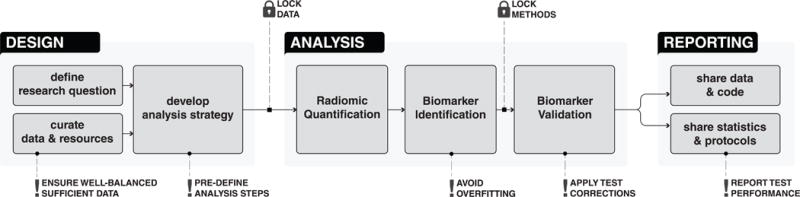
Design involves defining research scope and questions, curating the required data and resources and exploring and developing the analysis strategies. Analysis begins with radiomic quantification, followed by biomarker identification and validation. Data, code, and other details related to experiment are reported and shared during the Reporting stage.

Table 1. Recommendations for analyzing medical image data in radiology.

These recommendations cover different steps like Design, Analysis and Reporting.

Design: Define research question	-Define research questions -Review related literature and assess the scope of the research -Requirements gathering (required datasets, tools, etc.) -Feasibility assessment and timeline -Refine and finalize research questions and resource requirements
Design: Data and resource curation	-Gather and curate the required resources (data, tools) -Check the quality of imaging and clinical data and perform the appropriate selection
Design: Develop analysis strategy	-Based on available data, define the suitable analysis strategies - Explore and decide the suitable methods and computational approaches: - Feature quantification (engineered vs. deep learning) - Image preprocessing - Data normalization - Supervised vs. unsupervised - Dimensionality reduction - Statistical modeling -Define the analysis flow and timeline -Fix the hypotheses and their evaluation strategies -Fix the training and validation cohorts and ensure no data leakage -Fix the resources to be used
Design: Strive for balance	-Assure that different phenotypic groups are represented appropriately in the training data.
Design: Lock Data	-Lock training and validation cohorts to avoid information leakage. -Ensure that validation data remains locked(unused) until the exploratory analysis and biomarker identification is done on training cohorts.
Analysis: Preprocessing	-Perform the required image pre-processing. -Assess potential batch effects between cohorts and apply correction methods if needed.
Analysis: Radiomic quantification	-Explore and fix the the feature quantification methods. Radiologic characteristics can be quantified, for example, using engineered or deep learned features. -Accordingly fix the feature transformation and data normalization approaches.
Analysis: Biomarker identification	-Explore the feature selection/reduction and machine learning/deep learning modeling approaches using the cross-validation of training cohorts. -Explore different parameter settings and tuning strategies using cross-validation of training data.
Analysis: Lock Methods	-All methods and parameters should be locked (fixed) before applying them to validation data. -A report, testifying that validation data was not seen during the training and exploratory analysis stage, should be sent to the institutional review board (IRB) along with the list of locked methods that will be applied on the validation cohort.
Analysis: Biomarker validation	-Evaluate performance of previously fixed methods in the validation data. -Perform multiple test corrections if applicable -Statistically compare the performance of identified biomarker with conventional clinical markers. -Also, evaluate the complementary additive effect of the identified biomarker on conventional clinical markers and test if there is a significant increase in the performance.
Reporting: Statistics and protocols	-Report all relevant information and parameters related to each statistical test, such as the number of features tested, uncorrected and corrected p-values, effect size, and a rationale for the choice of a model or test. -Report acquisition protocols of the imaging data. Also, report segmentation protocols if these were performed. -List all the software and tools used. -If space is an issue then these details can be provided as a supplementary information to the article or report.
Reporting: Share Data & Methods	-Share the data and methods to the scientific community if feasible. This often brings more reproducibility in science and also increases the overall impact of a publication.

Design: research definition, data curation, and strategic decisions

Experimental design should be defined from the outset of a study. An experienced statistician should be consulted from the beginning of the study. By anticipating big picture challenges, the research question should be defined, required resources and data be identified and curated, and ultimately high-level decisions related to analysis strategies should be made. (see Figure 1, Table 1).

Define Research Question

To begin with, the overall scope of the research and the potential impact in the field should be assessed by reviewing relevant scientific literature and consulting domain experts. Subsequently, feasibility of the study should be assessed and a tentative timeline should be established. If possible, effect sizes should be anticipated to assess whether additional data and resources would be required. Finally, the research questions to be investigated and the corresponding resource requirements should be defined.

Curate Data and Resources

During this step, imaging and clinical data should be gathered and curated, and access to computational resources and methods should be established. Careful curation and annotation of the imaging and clinical data is important for quality control (QC) of the data and analysis. Validated open-source software tools should be prefered over their proprietary commercial counterparts to increase reproducibility and interpretability. Moreover, if multiple analysts are working on the analysis, standardized computational platforms and software versions should be used to increase consistency and reproducibility. Researchers should strive for balance to assure that different phenotypic groups are represented appropriately in the training and validation data sets. Here, balance refers to the balanced proportion of different classes of outcome or target variables. In cases where class imbalance is inevitable, appropriate strategies like augmentation or bootstrapping can be utilized.

Develop Analysis Strategy

Once the scope is defined and the required data and resources are curated, important decisions related to analysis strategies should be made. Different computational approaches should be reviewed to identify suitable methods for the analysis of radiographic data. For example, feature quantification strategies (i.e. engineered features or deep learning), image preprocessing methods, data normalization approaches, dimensionality reduction and feature selection methods, as well as different supervised and unsupervised modeling approaches should all be explored for the exploratory empirical analysis. Another important aspect in this step is to define and lock (fix) the training and validation cohorts. Within the analysis stage, the training cohort can be used for the exploratory empirical analysis to further select and lock the computation methods. However, the validation data should be kept locked and untouched, until all methods are fixed in the analysis phase (see Figure 1). Locked validation data will prevent information leakage from training to validation and limit the possibility of overfitting.

A commonly observed pitfall (see Table 2) that can be avoided at the design stage is when the number of samples is realistically too low to attain significance or to train a model. Insufficient training data could diminish the learning capability of a model, whereas insufficient validation data hinders the true evaluation of the underlying hypotheses. In this case, it might be best to gather more data samples, investigate only more conservative questions, or postpone the study until a later time. While seemingly undesirable, calling off a study at the design stage is preferable rather than investing time and effort in a study that is premature or underpowered to achieve statistical significance. Such a premature analysis can lead to overfitting as researchers scramble to find a combination of analysis choices that give “publishable” numbers.

Table 2. Commonly observed pitfalls.

A list of commonly observed pitfalls in data analysis of medical image data.

Pitfall 1: No predefined analysis protocol	-Not defining the analysis protocols beforehand could result in testing a large number of different design strategies to optimize the performance, which often does not generalize to other independent data sets.
Pitfall 2: Insufficient data for training and validation	-Insufficient training data could diminish the learning capability of a model. Insufficient validation data hinders the true evaluation of the underlying hypotheses.
Pitfall 3: No multiple test correction	-When a large number of features are statistically evaluated, often there is a chance of false “discovery”. Several statistical techniques, known as multiple testing corrections, are available to prevent that. No (or incorrect) multiple testing correction could induce erroneous statistical inferences and results.
Pitfall 4: No feature reduction	-Large number of features increase the chance of false “discovery”. Moreover, it could also induce the multicollinearity and overfitting. Therefore in order to avoid the curse of dimensionality, feature reduction or selection methods are required.
Pitfall 5: Overfitting	-While an overfitted model works extremely well in the initial training data set, its performance degrades substantially on other, independent data sets. Proper strategies should be applied to reduce the chance of overfitting on training data.
Pitfall 6: No locked data and Information leakage	-Often validation (parts of) data is used within training procedure. For example, features are selected based on the complete dataset, including validation data, and then these features are used for training a model in the training data. Validating this model in the validation cohort would be incorrect. As features are selected using the validation cohort, there is a possibility of information leakage and overfitting. Similarly, validation data can not be used for tuning the hyperparameters. Validation data should always be locked and untouched during training.
Pitfall 7: Not reporting appropriate performance metric	-Often using a single performance metric for the evaluation of a model is not sufficient. For example, accuracy of a classifier is sensitive to the event ratio (class distribution) of a population. Accurate evaluation can be achieved by reporting multiple performance metrics. For example, in classification studies, AUC, Sensitivity, Specificity, PPV, NPV etc. should be reported along with the accuracy of a classifier.
Pitfall 8: Training performance are incorrectly reported	-Often it has been observed that model performance on the training data is reported as results. Although this could provide information regarding the learning capability and convergence of a model, it does not give any information regarding the generalizability of a model and hence does not allow valid evaluation. Results should only emphasise the model performance in the independent validation cohorts.

Analysis: Preprocessing

In the second phase, the analysis is initiated with the goal of quantifying radiologic characteristics and ultimately establishing and validating imaging biomarkers (see Figure 2). When analyzing radiological cohorts, some preprocessing is required to reduce technical variability across images. Different sources of batch variability should be investigated, including difference in scanning instrumentations, signal drifts and other calibration-related issues as well as longitudinal effects and changes in imaging protocols. Statistical methods to correct for such batch effects should be applied. These steps ensure true assessment and validation of the underlying hypotheses.

Figure 2. Detailed analysis stage.

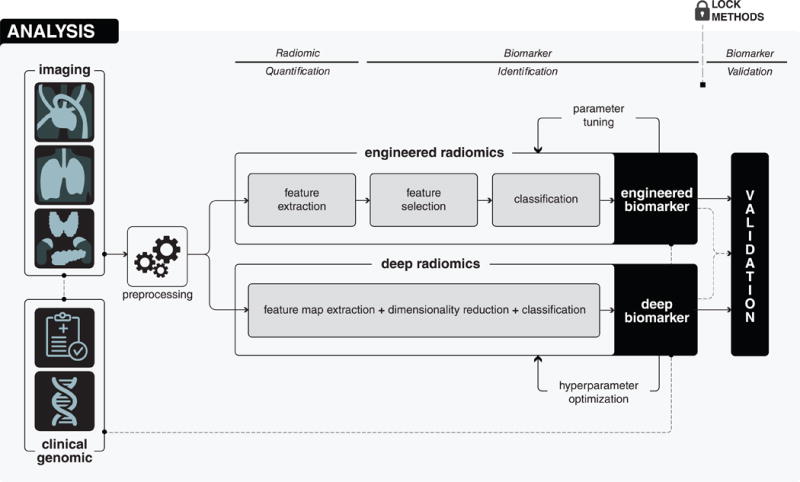
Analysis begins with the preprocessing of medical images in order to avoid different technical variability and batch effects. After that, in the radiomic quantification step, radiomic descriptors, capturing different phenotypic characteristics of diseased tissues are quantified. Radiomic quantification can either be done using engineered features or deep learning methods. According to the quantification method, in the biomarker identification step, appropriate analysis methods are explored and suitable methods are applied to develop biomarkers. Finally, in the biomarker validation step, the developed biomarker is validated in the locked and independent validation cohort.

Examples of image pre-processing prior to feature quantification include resampling of dimensions to isometric voxels to homogenize image resolutions. Images with isometric voxel dimensions can be either reconstructed from the raw DICOM data or interpolated from the image data. Moreover, some modalities such as MRI, require normalization of image intensity values. Sources of variability and image normalization steps are critical correction measures for imaging-related batch effects.

Analysis: Radiomic Quantification

Within radiology, AI methods can perform comprehensive quantifications of tissue characteristics (see Figure 2). These methods can convert 3D radiological images into high dimensional phenotype descriptors. This approach, called radiomics, uses engineered features and/or deep learning. Here, we will describe these two approaches independently.

Engineered Features

Engineered features are predefined and hard-coded algorithms designed to quantify specific radiographic characteristics of diseased tissues(7). Domain-specific expertise can be used to identify important phenotypic characteristics of diseased tissues, which could then be mathematically defined and programmatically extracted in an automated manner. For example, nodular ground glass opacity is considered as one of the vital factor for the management of pulmonary nodules(23,24). This domain specific knowledge has been used to define different statistical features (i.e. mean, median, variance, range etc.) from the intensity distributions of the nodules(7). It has been shown that the ground glass nodules have significantly lower median intensity values than partly solid or solid nodules(25). Similarly, it has been demonstrated that different radiomic features based on the shape, texture and regional heterogeneity of the diseased tissues, are associated with several clinical endpoints in oncology(4,10,11,13,25–32), and also in other domains such as cardiology(14).

Additional data normalization steps like feature transformation and standardization are needed for engineered features due to the intrinsic differences of range, scale and statistical distributions of these features. Untransformed features may have high levels of skewness which tend to result in artificially low p-values in downstream statistical tests for low sample size cohorts. Neglecting feature standardization may lead to individual features being over- or under-represented in statistical models and eventually introduce bias into the analysis. Methods like standardization and logarithmic transformations(33) can transform features into zero-centered distributions having identical variances and symmetric distributions.

Deep learning

Deep learning enables the extraction of multiple feature levels from data directly without explicit definition(8,34,35). It provides a higher level of feature abstraction and thus potentially providing better prediction performance. While deep learning has recently achieved impressive successes in practice, a strong theoretical backing is yet to be established(36). The lack of “rules of thumb” makes choosing an appropriate deep learning network architecture challenging. The problem at hand: classification, detection, segmentation, registration or reconstruction, in addition to the type and size of data, all hint at the appropriate architecture to utilize. Starting from published architectures that have proven successful in their respective tasks is common practice. Convolutional neural networks (CNNs) are the most prevalent deep learning architectures in medical imaging today(37). Transfer learning, or using pre-trained networks, is often an attractive option when dealing with scarce data(38). Data normalization is an essential data preprocessing step for deep learning. It ensures increased numerical stability and quicker and stable convergence. This could be achieved through sample-wise, feature-wise, or PCA whitening normalization depending on the data type. It is important to note, however, that even with inputs being normalized, their distributions are highly susceptible to change as they propagate through the network where parameters are constantly optimized during training - a problem referred to as “internal covariance shift”, and can be mitigated using batch normalization(39) or layer normalization(40). Normalization is hence made to be an integral part of the network architecture, as opposed to merely being a preprocessing step, and is performed on inputs to each layer, based on the distribution of the given batch of cases.

A few important points should be considered before choosing the quantification method. While deep learning is able to perform quantifications in an automated manner, it generally requires fairly large datasets. Often with quantitative imaging, it could be challenging to gather and curate large cohorts of patients with similar clinical, imaging and demographic characteristics. Engineered features are less sensitive to the cohort size but need to be defined manually by experts. Moreover, it also requires the segmentation of the diseased tissue. Recent efforts utilizing transfer learning have broadened the applicability of deep learning approaches to smaller cohorts(38,41). Hence, these points should be carefully considered prior to choosing a particular quantification method.

Analysis: Biomarker Identification

Quantitative analysis of medical image data involves mining large number of imaging features, with the goal of identifying highly predictive/prognostic biomarkers. Here, we discuss these concepts for engineered features and deep learning methods separately.

Engineered Features

A large number of engineered features are extracted from the medical image data, which might be highly redundant. The use of appropriate feature selection/reduction strategies can minimize the feature redundancies and mitigate the “curse of dimensionality”(42). Many unsupervised and supervised feature selection methods have been described in the literature(10). Unsupervised methods based on principal component analysis, independent component analysis, or correlation, can reduce the feature space without using a target outcome. Alternatively, supervised methods can be used to select features that are relevant to the particular target outcome(43,44). These supervised methods can be categorised into three categories: wrapper, embedded and filter methods. Computationally expensive wrapper and embedded methods use stricter model structure assumptions and are likely to have low generalizability, whereas model independent filter methods are relatively efficient and provide better generalizability(43,44).

Predictive and prognostic models with high accuracy, reliability, and efficiency are vital factors driving the success of quantitative imaging approaches(10). Myriad supervised and unsupervised methods exist in the machine learning literature derived using different statistical assumptions(42,45,46). Several investigations have compared these methods for quantitative image analyses(47–49),(10. These studies have demonstrated that the variability of prediction scores is highly influenced by method choice(10,42). Therefore, the choice of feature selection and machine learning modeling methods should be cautiously made.

One of the most commonly observed pitfalls during biomarker identification stage is overfitting. Researchers have a tendency to exhaustively search through different modeling methods and parameter configurations to obtain high and publishable performance, which can result in poor biomarker generalizability. To avoid this, use of standard settings for hyperparameters(50) or locked and independent validation data(51) is recommended.

Deep learning

In deep learning, dimensionality reduction and classification are performed alongside feature extraction in an integrated manner (see Figure 2). However, the quality and output of these cascaded layers depend on different hyperparameters such as the number of layers and feature maps, layer arrangement and architecture, size of the receptor field etc. Many different network architectures have been described using different sets of hyperparameters(52,53). Prediction performance could be influenced by the choice of these hyperparameters and architectures. As in the case of engineered features, optimizing the hyperparameters by exhaustively searching the parameter space, is a common pitfall in deep learning as well. The deep learning architecture should be selected based on the underlying scope and application of the research, the statistical properties of data in hand, and the effective data size.

Overfitting represents a major challenge in deep learning and can drastically affect a network’s ability to generalize to unseen data. Often, deep learning methods are treated as a “black box” and not enough attention is given to understanding the actual methods and technical concepts. This is particularly an issue when working with limited training data. Deeper and more complex networks trained on limited data could induce overfitting. The use of shallower networks could avoid overfitting but may result in insufficient learning, also known as underfitting. One solution could be data augmentation, where the training data is expanded by applying label-preserving image transformations(54) like cropping, reflections and rotations. Dropout or other regularization methods could also be used to reduce overfitting(55,56). Dropout makes the network less sensitive to individual weights and hence increases the robustness of a network. Other regularization methods allow penalizing large parametric weights to make the network more robust and generalizable. During training, the network performance should be evaluated and monitored using cross-validation. A cross validation-based early stopping(57) approach can also be utilized to avoid overfitting. These important factors should be considered during the biomarker identification stage.

After identifying biomarkers, a document should be created listing all the cross-validation and analysis steps taken during the exploratory analysis of training data, the final hypotheses to be validated, the training data used and corresponding inclusion criteria, as well as a list of identified and locked computational approaches. Furthermore, it should also be declared that the validation data was not used during the exploratory analysis or biomarker identification stage. The same document can later be used to incorporate validation results and reported alongside the study findings.

Analysis: Biomarker Validation

As described in the previous sections, avoiding overfitting and data leakage is essential when working with machine learning and deep learning models. It should be ensured that locked validation cohorts remain blinded during the training and hyperparameter tuning. Only after fixing the models, network architectures, computational methods, and corresponding hyperparameters, should the validation be carried out on the locked validation cohorts. These steps ensure the true evaluation of the underlying hypotheses.

Appropriate performance metrics should be used, especially, when dealing with highly unbalanced classes. For example, the accuracy of a classifier is potentially sensitive to the event ratio (class distribution) of a population resulting in deceivingly over-optimistic results. Accurate evaluation can be achieved by reporting multiple performance metrics like AUC, Sensitivity, Specificity, Positive Predictive Value, Negative Predictive Value etc. Moreover, robustness of the biomarkers with respect to data perturbation is also a vital aspect of biomarker validation(58). An essential and often overlooked step before choosing candidate biomarkers is performing multiple testing corrections. When testing hundreds of features, it is expected that some associations with clinical outcomes can be found entirely by chance. To avoid this, correction methods like Bonferroni(59) and Benjamini and Hochberg(60) should be applied.

In order to gage the true clinical impact, it is also essential to statistically compare the developed biomarkers to standard clinical markers during validation. Furthermore, the additive increase in performance should also be evaluated by combining the developed biomarkers and standard clinical markers in a computational model. Moreover, emphasis should be given to multiple external validation sets, which can ensure the robustness and generalizability of a biomarker. It is our view that studies demonstrating biomarker robustness through reproducibility should be looked upon favorably.

Sharing and Reporting

In the final phase, a detailed report should be made about the data, analysis methods, and results. Furthermore, enough emphasis should be given to sharing the analysis protocols, documented code, original as well as processed data, along with detailed descriptions.

Share data and code

There are several technical and privacy issues to be considered while sharing biomedical imaging data. Patient confidentiality must be protected throughout the entire process. A system similar to that of the database of Genotypes and Phenotypes(dbGaP) should be adopted, where raw imaging data can be archived and distributed in a manner that enables data sharing without compromising patient confidentiality. Publicly available online medical imaging repository, The Cancer Imaging Archive (TCIA) (http://www.cancerimagingarchive.net/), is a great place for sharing and archiving medical image data as it uses a standards-based approach to de-identification of DICOM images to insure that images are free of protected health information (PHI). For analysis, repositories like GitHub (http://github.com) allow for relative ease in sharing code. Furthermore, computational tools such as Jupyter notebooks and Sweave can make “executable documents”, which should be included as supplements to the scientific articles to promote reproducibility and generalizability. Experiments housed in software environment containers with locked versioning such as docker (www.docker.com) allow for swift reproducibility and portability.

Share statistics & protocols

As building imaging biomarkers from radiological data involves multiple analytical steps, sharing comprehensive descriptions of statistical methods are essential for reproducibility. We recommend reporting the number of samples and features tested, feature definitions, the statistical tests and algorithms used during the analysis, list of model and hyper parameters used, details regarding the optimization methods, nominal and corrected p-values, and effect size assessments, in the shared document. Once imaging data has gone through the quantification steps outlined above, the result is normally a matrix of features versus samples. As long as sample labels are properly de-identified, this feature matrix can usually be shared without any risk to patient confidentiality. Ideally, all code required to reproduce study findings from the feature matrix should also be shared, with the exception of sections that require the use of protected clinical metadata.

An effective strategy often adopted for data sharing is to group data, analysis reports, and runnable code blocks into a single object such as R data packages with vignettes. For studies that use deep learning approaches, the type of network architecture and hyper parameters should be shared. Additionally, sharing entire networks with trained weights can be highly beneficial for transfer-learning efforts. With an increasing number of deep learning libraries, sharing trained networks in universal formats such as ONNX (www.onnx.ai) can facilitate straightforward cross-platform compatibility. It is our experience that sharing methods and code in this manner also has the natural effect of raising the overall quality of data analyses, in addition to ensuring reproducibility.

Data science and big data are rapidly becoming major components of healthcare applications in both the industrial and academic settings. However, performing accurate and meaningful data analyses is challenging and potentially plagued with errors and incorrect conclusions. In this article, we addressed data analyses practices specific to radiographic medical images. We identified commonly observed pitfalls and recommended vital guidelines. Recommendations given here are not exclusive solutions nor do they guarantee completely error-free unbiased experimentation. However, they do act as guidelines for the management and handling of research-compromising pitfalls. Mindful implementation of these guidelines will enhance the quality of radiomic analyses as well as allow for better integration of imaging data with other patient-specific data for precision medicine efforts.

References

- 1.Wang W, Krishnan E. Big data and clinicians: a review on the state of the science. JMIR Med Inform ncbi.nlm.nih.gov. 2014;2:e1. doi: 10.2196/medinform.2913. [DOI] [PMC free article] [PubMed] [Google Scholar]
- 2.Luo J, Wu M, Gopukumar D, Zhao Y. Big Data Application in Biomedical Research and Health Care: A Literature Review. Biomed Inform Insights ncbi.nlm.nih.gov. 2016;8:1–10. doi: 10.4137/BII.S31559. [DOI] [PMC free article] [PubMed] [Google Scholar]
- 3.Aerts HJWL. The Potential of Radiomic-Based Phenotyping in Precision Medicine: A Review. JAMA Oncol [Internet] 2016 doi: 10.1001/jamaoncol.2016.2631. oncology.jamanetwork.com; Available from: [DOI] [PubMed]
- 4.Aerts HJWL, Velazquez ER, Leijenaar RTH, Parmar C, Grossmann P, Carvalho S, et al. Decoding tumour phenotype by noninvasive imaging using a quantitative radiomics approach. Nat Commun. 2014;5:4006. doi: 10.1038/ncomms5006. [DOI] [PMC free article] [PubMed] [Google Scholar]
- 5.Kumar V, Gu Y, Basu S, Berglund A, Eschrich SA, Schabath MB, et al. Radiomics: the process and the challenges. Magn Reson Imaging Elsevier. 2012;30:1234–48. doi: 10.1016/j.mri.2012.06.010. [DOI] [PMC free article] [PubMed] [Google Scholar]
- 6.Lambin P, Rios-Velazquez E, Leijenaar R, Carvalho S, van Stiphout RGPM, Granton P, et al. Radiomics: extracting more information from medical images using advanced feature analysis. Eur J Cancer. 2012;48:441–6. doi: 10.1016/j.ejca.2011.11.036. [DOI] [PMC free article] [PubMed] [Google Scholar]
- 7.van Griethuysen JJM, Fedorov A, Parmar C, Hosny A, Aucoin N, Narayan V, et al. Computational Radiomics System to Decode the Radiographic Phenotype. Cancer Res AACR. 2017;77:e104–7. doi: 10.1158/0008-5472.CAN-17-0339. [DOI] [PMC free article] [PubMed] [Google Scholar]
- 8.LeCun Y, Bengio Y, Hinton G. Deep learning. Nature nature.com. 2015;521:436–44. doi: 10.1038/nature14539. [DOI] [PubMed] [Google Scholar]
- 9.Rusk N. Deep learning. Nat Methods. 2015;13:35–35. [Google Scholar]
- 10.Parmar C, Grossmann P, Bussink J, Lambin P, Aerts HJWL. Machine Learning methods for Quantitative Radiomic Biomarkers. Sci Rep. 2015;5:13087. doi: 10.1038/srep13087. [DOI] [PMC free article] [PubMed] [Google Scholar]
- 11.Coroller TP, Grossmann P, Hou Y, Rios Velazquez E, Leijenaar RTH, Hermann G, et al. CT-based radiomic signature predicts distant metastasis in lung adenocarcinoma. Radiother Oncol Elsevier. 2015;114:345–50. doi: 10.1016/j.radonc.2015.02.015. [DOI] [PMC free article] [PubMed] [Google Scholar]
- 12.Wu W, Parmar C, Grossmann P, Quackenbush J, Lambin P, Bussink J, et al. Exploratory Study to Identify Radiomics Classifiers for Lung Cancer Histology. Front Onco ncbi.nlm.nih.gov. 2016;6:71. doi: 10.3389/fonc.2016.00071. [DOI] [PMC free article] [PubMed] [Google Scholar]
- 13.Huynh E, Coroller TP, Narayan V, Agrawal V, Romano J, Franco I, et al. Associations of Radiomic Data Extracted from Static and Respiratory-Gated CT Scans with Disease Recurrence in Lung Cancer Patients Treated with SBRT. PLoS One. 2017;12:e0169172. doi: 10.1371/journal.pone.0169172. [DOI] [PMC free article] [PubMed] [Google Scholar]
- 14.Kolossváry M, Kellermayer M, Merkely B, Maurovich-Horvat P. Cardiac Computed Tomography Radiomics: A Comprehensive Review on Radiomic Techniques. J Thorac Imaging [Internet] 2017 doi: 10.1097/RTI.0000000000000268. Available from: [DOI] [PubMed]
- 15.O’Connor JPB, Aboagye EO, Adams JE, Aerts HJWL, Barrington SF, Beer AJ, et al. Imaging biomarker roadmap for cancer studies. Nat Rev Clin Oncol. 2017;14:169–86. doi: 10.1038/nrclinonc.2016.162. [DOI] [PMC free article] [PubMed] [Google Scholar]
- 16.Quackenbush J. Microarray data normalization and transformation. Nat Genet. 2002;32:496–501. doi: 10.1038/ng1032. [DOI] [PubMed] [Google Scholar]
- 17.Leek JT, Scharpf RB, Bravo HC, Simcha D, Langmead B, Johnson WE, et al. Tackling the widespread and critical impact of batch effects in high-throughput data. Nat Rev Genet. 2010;11:733–9. doi: 10.1038/nrg2825. [DOI] [PMC free article] [PubMed] [Google Scholar]
- 18.Johnson WE, Li C, Rabinovic A. Adjusting batch effects in microarray expression data using empirical Bayes methods. Biostatistics. 2007;8:118–27. doi: 10.1093/biostatistics/kxj037. [DOI] [PubMed] [Google Scholar]
- 19.Lee ML, Kuo FC, Whitmore GA, Sklar J. Importance of replication in microarray gene expression studies: statistical methods and evidence from repetitive cDNA hybridizations. Proc Natl Acad Sci U S A. 2000;97:9834–9. doi: 10.1073/pnas.97.18.9834. [DOI] [PMC free article] [PubMed] [Google Scholar]
- 20.Neve RM, Chin K, Fridlyand J, Yeh J, Baehner FL, Fevr T, et al. A collection of breast cancer cell lines for the study of functionally distinct cancer subtypes. Cancer Cell. 2006;10:515–27. doi: 10.1016/j.ccr.2006.10.008. [DOI] [PMC free article] [PubMed] [Google Scholar]
- 21.Allison DB, Cui X, Page GP, Sabripour M. Microarray data analysis: from disarray to consolidation and consensus. Nat Rev Genet. 2006;7:55–65. doi: 10.1038/nrg1749. [DOI] [PubMed] [Google Scholar]
- 22.Aerts HJ. Clin Cancer Res [Internet] AACR; 2017. Data Science in Radiology: A Path Forward. Available from: [DOI] [PMC free article] [PubMed] [Google Scholar]
- 23.Lee C-T. What do we know about ground-glass opacity nodules in the lung? Transl Lung Cancer Res. 2015;4:656–9. doi: 10.3978/j.issn.2218-6751.2015.04.05. [DOI] [PMC free article] [PubMed] [Google Scholar]
- 24.de Hoop B, Gietema H, van de Vorst S, Murphy K, van Klaveren RJ, Prokop M. Pulmonary Ground-Glass Nodules: Increase in Mass as an Early Indicator of Growth. Radiology Radiological Society of North America. 2010;255:199–206. doi: 10.1148/radiol.09090571. [DOI] [PubMed] [Google Scholar]
- 25.Yip SSF, Liu Y, Parmar C, Li Q, Liu S, Qu F, et al. Associations between radiologist-defined semantic and automatically computed radiomic features in non-small cell lung cancer. Sci Rep nature.com. 2017;7:3519. doi: 10.1038/s41598-017-02425-5. [DOI] [PMC free article] [PubMed] [Google Scholar]
- 26.Nie K, Chen J-H, Yu HJ, Chu Y, Nalcioglu O, Su M-Y. Quantitative analysis of lesion morphology and texture features for diagnostic prediction in breast MRI. Acad Radiol. 2008;15:1513–25. doi: 10.1016/j.acra.2008.06.005. [DOI] [PMC free article] [PubMed] [Google Scholar]
- 27.Kalpathy-Cramer J, Mamomov A, Zhao B, Lu L, Cherezov D, Napel S, et al. Radiomics of Lung Nodules: A Multi-Institutional Study of Robustness and Agreement of Quantitative Imaging Features. Tomography. 2016;2:430–7. doi: 10.18383/j.tom.2016.00235. [DOI] [PMC free article] [PubMed] [Google Scholar]
- 28.Jain R, Poisson LM, Gutman D, Scarpace L, Hwang SN, Holder CA, et al. Outcome prediction in patients with glioblastoma by using imaging, clinical, and genomic biomarkers: focus on the nonenhancing component of the tumor. Radiology. 2014;272:484–93. doi: 10.1148/radiol.14131691. [DOI] [PMC free article] [PubMed] [Google Scholar]
- 29.Bae JM, Jeong JY, Lee HY, Sohn I, Kim HS, Son JY, et al. Pathologic stratification of operable lung adenocarcinoma using radiomics features extracted from dual energy CT images. Oncotarget. 2017;8:523–35. doi: 10.18632/oncotarget.13476. [DOI] [PMC free article] [PubMed] [Google Scholar]
- 30.Grossmann P, Stringfield O, El-Hachem N, Bui MM, Rios Velazquez E, Parmar C, et al. Defining the biological basis of radiomic phenotypes in lung cancer. Elife [Internet] 2017:6. doi: 10.7554/eLife.23421. Available from: [DOI] [PMC free article] [PubMed]
- 31.Rios Velazquez E, Parmar C, Liu Y, Coroller TP, Cruz G, Stringfield O, et al. Somatic mutations drive distinct imaging phenotypes in lung cancer. Cancer Res [Internet] 2017 doi: 10.1158/0008-5472.CAN-17-0122. Available from: [DOI] [PMC free article] [PubMed]
- 32.Parmar C, Leijenaar RTH, Grossmann P, Rios Velazquez E, Bussink J, Rietveld D, et al. Radiomic feature clusters and prognostic signatures specific for Lung and Head & Neck cancer. Sci Rep nature.com. 2015;5:11044. doi: 10.1038/srep11044. [DOI] [PMC free article] [PubMed] [Google Scholar]
- 33.Huber W, von Heydebreck A, Sültmann H, Poustka A, Vingron M. Variance stabilization applied to microarray data calibration and to the quantification of differential expression. Bioinformatics. 2002;18(Suppl 1):S96–104. doi: 10.1093/bioinformatics/18.suppl_1.s96. [DOI] [PubMed] [Google Scholar]
- 34.Miotto R, Wang F, Wang S, Jiang X, Dudley JT. Deep learning for healthcare: review, opportunities and challenges. Brief Bioinform [Internet] 2017 doi: 10.1093/bib/bbx044. Available from: [DOI] [PMC free article] [PubMed]
- 35.Kevin Zhou S, Greenspan H, Shen D. Deep Learning for Medical Image Analysis. Academic Press; 2017. [Google Scholar]
- 36.Wang G. A Perspective on Deep Imaging. IEEE Access. 2016;4:8914–24. [Google Scholar]
- 37.Litjens G, Kooi T, Bejnordi BE, Setio AAA, Ciompi F, Ghafoorian M, et al. A Survey on Deep Learning in Medical Image Analysis [Internet] arXiv [cs.CV] 2017 doi: 10.1016/j.media.2017.07.005. Available from: http://arxiv.org/abs/1702.05747. [DOI] [PubMed]
- 38.Shin H-C, Roth HR, Gao M, Lu L, Xu Z, Nogues I, et al. Deep Convolutional Neural Networks for Computer-Aided Detection: CNN Architectures, Dataset Characteristics and Transfer Learning. IEEE Trans Med Imaging. ieeexplore.ieee.org. 2016;35:1285–98. doi: 10.1109/TMI.2016.2528162. [DOI] [PMC free article] [PubMed] [Google Scholar]
- 39.Ioffe S, Szegedy C. Batch Normalization: Accelerating Deep Network Training by Reducing Internal Covariate Shift [Internet] arXiv [cs.LG] 2015 Available from: http://arxiv.org/abs/1502.03167.
- 40.Ba JL, Kiros JR, Hinton GE. Layer Normalization [Internet] arXiv [stat.ML] 2016 Available from: http://arxiv.org/abs/1607.06450.
- 41.Weiss K, Khoshgoftaar TM, Wang D. A survey of transfer learning. Journal of Big Data [Internet] 2016;3 doi: 10.1186/s40537-016-0043-6. Available from: [DOI] [Google Scholar]
- 42.Hastie T, Tibshirani R, Friedman J. The Elements of Statistical Learning: Data Mining, Inference, and Prediction. Springer Science & Business Media; 2013. [Google Scholar]
- 43.Guyon I, Elisseeff A. An Introduction to Variable and Feature Selection. J Mach Learn Res jmlr.org. 2003;3:1157–82. [Google Scholar]
- 44.Brown G, Pocock A, Zhao M-J, Luján M. Conditional Likelihood Maximisation: A Unifying Framework for Information Theoretic Feature Selection. J Mach Learn Res jmlr.org. 2012;13:27–66. [Google Scholar]
- 45.Mohri M, Rostamizadeh A, Talwalkar A. Foundations of Machine Learning. MIT Press; 2012. [Google Scholar]
- 46.Fernández-Delgado M, Cernadas E, Barro S. Do we need hundreds of classifiers to solve real world classification problems. J Mach Learn Res [Internet]. jmlr.org. 2014 Available from: http://www.jmlr.org/papers/volume15/delgado14a/source/delgado14a.pdf.
- 47.El Naqa I, Li R, Murphy MJ. Machine Learning in Radiation Oncology: Theory and Applications. Springer; 2015. [Google Scholar]
- 48.Wang J, Wu C-J, Bao M-L, Zhang J, Wang X-N, Zhang YD. Machine learning-based analysis of MR radiomics can help to improve the diagnostic performance of PI-RADS v2 in clinically relevant prostate cancer. Eur Radiol [Internet] 2017 doi: 10.1007/s00330-017-4800-5. Available from: [DOI] [PubMed]
- 49.Zhang B, He X, Ouyang F, Gu D, Dong Y, Zhang L, et al. Radiomic machine-learning classifiers for prognostic biomarkers of advanced nasopharyngeal carcinoma. Cancer Lett [Internet] 2017 doi: 10.1016/j.canlet.2017.06.004. Available from: [DOI] [PubMed]
- 50.Parmar C, Grossmann P, Rietveld D, Rietbergen MM, Lambin P, Aerts HJWL. Radiomic Machine-Learning Classifiers for Prognostic Biomarkers of Head and Neck Cancer. Front Oncol ncbi.nlm.nih.gov. 2015;5:272. doi: 10.3389/fonc.2015.00272. [DOI] [PMC free article] [PubMed] [Google Scholar]
- 51.Skocik M, Collins J, Callahan-Flintoft C, Bowman H, Wyble B. I TRIED A BUNCH OF THINGS THE DANGERS OF UNEXPECTED OVERFITTING IN CLASSIFICATION [Internet] 2016 doi: 10.1101/078816. Available from: [DOI] [PubMed]
- 52.Bengio Y, Courville A, Vincent P. Representation learning: a review and new perspectives. IEEE Trans Pattern Anal Mach Intell. 2013;35:1798–828. doi: 10.1109/TPAMI.2013.50. [DOI] [PubMed] [Google Scholar]
- 53.Schmidhuber J. Deep learning in neural networks: an overview. Neural Netw. 2015;61:85–117. doi: 10.1016/j.neunet.2014.09.003. [DOI] [PubMed] [Google Scholar]
- 54.Krizhevsky A, Sutskever I, Hinton GE. ImageNet Classification with Deep Convolutional Neural Networks. In: Pereira F, Burges CJC, Bottou L, Weinberger KQ, editors. Advances in Neural Information Processing Systems 25. Curran Associates, Inc; 2012. pp. 1097–105. [Google Scholar]
- 55.Bell RM, Koren Y. SIGKDD Explor Newsl. Vol. 9. New York, NY, USA: ACM; 2007. Lessons from the Netflix Prize Challenge; pp. 75–9. [Google Scholar]
- 56.Srivastava N, Hinton GE, Krizhevsky A, Sutskever I, Salakhutdinov R. Dropout: a simple way to prevent neural networks from overfitting. J Mach Learn Res. 2014;15:1929–58. [Google Scholar]
- 57.Prechelt L. Early Stopping - But When? In: Orr GB, Müller K-R, editors. Neural Networks: Tricks of the Trade. Springer Berlin Heidelberg; 1998. pp. 55–69. [Google Scholar]
- 58.Beck AH, Knoblauch NW, Hefti MM, Kaplan J, Schnitt SJ, Culhane AC, et al. Significance Analysis of Prognostic Signatures. PLoS Comput Biol. 2013;9:e1002875. doi: 10.1371/journal.pcbi.1002875. [DOI] [PMC free article] [PubMed] [Google Scholar]
- 59.Bonferroni CE. Teoria statistica delle classi e calcolo delle probabilità. 1936 [Google Scholar]
- 60.Benjamini Y, Hochberg Y. Controlling the False Discovery Rate: A Practical and Powerful Approach to Multiple Testing. J R Stat Soc Series B Stat Methodol. 1995;57:289–300. [Google Scholar]