Gradient‐echo EPI using a high‐degree shim insert coil at 7 T: Implications for BOLD fMRI

Abstract

Purpose

To quantitatively assess the effects of high degree and order (1^st–4^th+) relative to 1^st–2^nd degree B ₀ shimming at 7 Tesla (T) on gradient‐echo echo planar imaging (GE‐EPI) and blood‐oxygen‐level dependent (BOLD) activation.

Methods

Simulations and GE‐EPI were performed at (2mm)³ and (3mm)³ resolution, evaluating the temporal signal‐to‐noise ratio (tSNR), transverse relaxivity ( ${\mathrm{R}}_2^{*}$), BOLD % signal change and activated pixel counts in a breath‐hold task.

Results

Comparing the 1^st–4^th+ degree with 1^st–2^nd degree shimmed B ₀ maps generated spatially varying regions of $\Delta \left|B_0\right|=\left|B_0^{1-2}\right|-\left|B_0^{1-4+}\right|$. As binned in 10‐Hz intervals, the two center Δ|B ₀| (±10 Hz) bins maintained the B ₀ offset of 48.6% of gray‐matter pixels. In the positive Δ|B ₀| bins greater than 10 Hz, the 1^st–4^th+degree shimming improved the B ₀ offset in 41.1%; in negative Δ|B ₀| bins less than −10 Hz, the offset worsened in 10.2% of the pixels. In the positive Δ|B ₀| bins, we found variable but significant increases in BOLD sensitivity; the negative Δ|B ₀| bins showed significant decreases. In the breath‐hold studies, positive bins showed significantly increased activated pixel numbers (+5–29%), whereas negative bins showed −18 to 0% decline.

Conclusion

1^st–4^th+ degree shimming maintained B ₀ homogeneity over central brain regions while improving most of the other regions, including the inferior frontal lobe. Magn Reson Med 78:1734–1745, 2017. © 2016 The Authors Magnetic Resonance in Medicine published by Wiley Periodicals, Inc. on behalf of International Society for Magnetic Resonance in Medicine. This is an open access article under the terms of the Creative Commons Attribution NonCommercial License, which permits use, distribution and reproduction in any medium, provided the original work is properly cited and is not used for commercial purposes.

INTRODUCTION

Functional magnetic resonance imaging (fMRI) is commonly performed by gradient‐echo (GE) echo planar imaging (EPI) because of its high sensitivity to blood oxygenation level dependent (BOLD) signal changes. However, EPI acquisitions are also known (much more than structural imaging) to be sensitive to the macroscopic field inhomogeneity generated by the differences in magnetic susceptibility in areas of heterogeneous tissues (including gray, white matter, or cerebrospinal fluid (CSF)) or at the boundary of air and tissue. With such local susceptibility variation, it is not surprising that smaller target regions (eg, parietal or occipital lobe) are generally less problematic for B ₀ inhomogeneity in comparison to the entire brain. These B ₀ variations, whether local or global, also directly affect the EPI. Although local B ₀ inhomogeneity with ${\mathrm{T}}_2^{*}$ weighting results in intravoxel dephasing and signal loss, the frequency offset from the carrier with EPI encoding results in pixel shifting, causing both signal distortion and loss. The resulting inaccurate registration between EPI data and high‐resolution anatomical images can lead to misinterpretation of the results.

Given these issues, it is useful to consider the state of the art in postprocessing and acquisition to improve B ₀ homogeneity. The commonly used pixel shift correction is known to improve overall appearance; however, such corrections can change image intensity 1, 2. Thin slices and z‐shimming can improve image quality 3, 4, 5, 6, but they reduce temporal resolution. Tailored radiofrequency (RF) pulses that compensate for susceptibility‐induced phase distortions require lengthy pulse trains and also result in limited slice numbers 7, 8. More direct improvements of field homogeneity have also been proposed, including active and passive shimming 9, 10, 11, 12, dynamic updating 13, 14, 15, 16, 17, and most recently, the use of multiple local coils 18, 19, 20. Wilson used diamagnetic mouth inserts to reduce B ₀ inhomogeneity from the inferior frontal lobe 10. Although it is effective at reducing B ₀ inhomogeneity from this region, the presence of the mouth insert increased head motion and salivation, degrading activation from the insula 11. To better tailor the correction field, Koch used a matrix of diamagnetic and paramagnetic shims, providing both positive and negative fields, arranged about the head 12. However, optimal placement of the passive shims is done outside of the magnet and requires an existing B ₀ map of the subject, necessitating a minimum of two different magnet sessions.

As stated, shimming a restricted target region can achieve both greater global and local homogeneity in the target (commonly with degradation in other regions) in comparison to shimming a larger overall region. Taking advantage of this effect, several groups 13, 14, 15, 16 have developed dynamic updating of the B ₀ shims for individual slices, reporting significant gains. More recently, the dynamic updating approach has been further developed with local shim coils 18, 19, 20 in which the shim coils are placed within the diameter of the RF shield or integrated with the RF coil itself. Although early results from this work are promising for slice‐by‐slice homogeneity, there have been fewer data on its performance in simultaneous whole‐brain shimming. Given the importance of simultaneous multislice (SMS) EPI methods, with their advantages for acquisition speed, enhanced brain coverage and statistical power for fMRI 21, in this report we assess the performance of spherical harmonic shimming for simultaneous whole‐brain coverage. We perform a simulation analysis that evaluates the effects of high‐degree (up to 10th degree) spherical harmonic shimming for EPI data. We then experimentally assess this using a commercially available high‐degree shim insert coil (3rd, 4th, and two 5th‐degree shims, denoted as 1^st–4^th+ shims) and quantitatively evaluate the effect of improved B ₀ shimming on the EPI signal intensity and distortion at two spatial resolutions: (2mm)³ and (3mm)³. Finally, a breath‐hold BOLD activation study is performed to directly evaluate the effect of the high‐degree shimming.

The terminology of spherical harmonics varies among different disciplines. Our text uses the notation of Abramowitz and Stegun 22, Hillenbrand 23, and the NIST Digital Library of Mathematical Functions (http://dlmf.nist.gov), in which the radial power n is called the “degree,” and the periodicity in the azimuthal angle is termed “order.”

METHODS

Nine healthy subjects (ages 38.6 ± 12.7, 4 male) were studied using an 8‐channel parallel transmit 7 Tesla (T) Siemens system (Erlangen, Germany). Of these n = 9 subjects, 6 subjects participated in the low and high‐resolution EPI studies and 8 subjects participated in a breath‐hold study comparing 1^st–2^nd to 1^st–4^th+ degree shimming. Five subjects participated in both studies. All studies were approved according to the University of Pittsburgh Institutional Review Board.

Simulation

Simulations were performed to assess the effects of higher degree shims (Fig. 1). In this simulation, an anatomical mask (intensity 1.0 in all pixels) was used with an experimental B ₀ data set, acquired with 1^st–2^nd degree shims to provide a base map of B ₀ homogeneity at (2mm)³ resolution. This map was interpolated to (1mm)³ resolution with the remainder of the simulation performed at this resolution, assuming a homogeneous spin density, omitting intrinsic T₂ relaxation and coil effects. A (1mm)³ size is used, in which the B ₀ variation is taken to be linear (ie, its net phase precession is determined only by its mean B ₀ offset). Thus, for a pixel at location r, the complex transverse magnetization is given by

$${\mathrm{M}}_{+}^{\text{shim}\hspace{0.17em}\text{degree}}(\overrightarrow{r},\mathrm{t})=\text{exp}(-\text{iTE}{}^{*}\gamma \Delta B_0^{\text{shim}\hspace{0.17em}\text{degree}}(\overrightarrow{r}))\cdot {\mathrm{M}}_{\perp }(\overrightarrow{r},0),$$ (1)

Figure 1.

Simulations of the EPI signal with varying degree of spherical harmonic shimming. B ₀ maps and an anatomical mask of uniform signal intensity (1.0) was used to simulate signal dephasing and voxel shift for 2nd–10th degree while shimming a whole brain. (a) B ₀ maps from an inferior frontal lobe slice (identified by the line on the sagittal structural image), as shimmed with 2nd, 4th, 6th, and 10th degree shims. The numbers shown in (a) are the standard deviation of the field $\sigma B_0^{\text{Global}}$ at each shim degree. (b) Simulated signal dephasing performed at three voxel resolutions; xN indicates the n number of x1 voxels, x1, x8 or x27, showing the greater intravoxel dephasing in the larger voxel simulations. (c) Voxel shifting performed on the dephased images is largest in the x1 resolution image, generating both decreased and increased pixel intensity. The dynamic range of data is [0,3] but is displayed at [0,2] for clarity. At x8 and x27, the images in (c) show signal loss as a result of a combined effect from the dephasing and shifting, which decrease with higher degree shimming. In (d and e) data are parcellated into 12 gray‐matter anatomical groups. (d) Covariance of the signal in each parcel as a function of shim degree gives an estimate of the signal heterogeneity that arises from complex signal summation (without any dephasing and shifting, the ideal covariance is 0.0). (e) Direct assessment of shifting, showing the fraction of pixels that shift out of its parcel. In some parcels, more than 50% of the pixels shift out. Twelve regions of brain are parcellated, with greater signal dropout observed in the amygdala, hippocampus, orbitofrontal, and inferior temporal regions.

Pixels are then shifted (Δp) according to their (shimmed) B ₀ offset and a fixed echo spacing of 750 μs, Δp = ΔB ₀*Np*echo spacing, summing the complex intensities that move to a common spatial position. By using a fixed echo spacing, the overall millimeter shifts are matched among different spatial resolutions (although the absolute numbers of pixels shifted are not), making the effects of intravoxel dephasing and shift‐linked summation more readily identified. To accommodate submillimeter pixel shifts in the distorted images, the pixel intensity was linearly interpolated across two adjacent pixels. This simulation, performed at 1‐mm base voxel size, may underestimate the absolute signal loss. However, this analysis is not intended as an absolute signal match; rather, it is designed to assess the behavior of the higher‐degree shims on the echo planar image. The effects of 2nd through 10th degree shimming were simulated by applying the residual B ₀ map in Equation [1] (B ₀ maps calculated without limitations on the applied current).

At (1mm)³ resolution, the shifted complex signal gives rise to possible destructive or constructive interference, creating “collision” or “expansion”‐based signal distortion. With the larger voxel sizes, 8 and 27 1‐mm voxels are summed ( ${\sum }^8{e}^{-i\left(\stackrel{\rightharpoonup }{r},t\right)}$ and ${\sum }^{27}{e}^{-i\left(\stackrel{\rightharpoonup }{r},t\right)}$), calculating the magnitude signal as $\sqrt{Re{\left(M_{+}\right)}^2+Im{\left(M_{+}\right)}^2}$ and normalizing by the number of voxels (either 8 or 27), performed for each degree of B ₀ map. With the summation over the larger voxel sizes, destructive and constructive interference also occurs, generating a smoother (albeit distorted) average value. Finally, to assess how the individual regions lose or gain signal intensity through the collision process, the anatomical MPRAGE image was parcellated by FreeSurfer (image analysis suite (which is documented and freely available for download online, http://surfer.nmr.mgh.harvard.edu/)) to generate 12 different brain regions (separated into gray and white matter) and the resulting parcels analyzed for signal dropout and voxel shift.

B ₀ Shim Insert, Field Map, and Shimming

An 18‐channel shim insert coil with 38‐cm ID, 43cm OD, and 70‐cm length, 18.5 cm from patient end to magnetic center, consisting of 3rd, 4th, and two 5th‐degree shims (ZC4 and ZS4) with 10A shim supplies (Resonance Research, Billerica, MA USA) was used for high‐degree shimming, denoted as 1^st–4^th+ shimming. The B ₀ field was mapped using the B ₀ loop encoded readout (Bolero) method 24, 25. In brief, the Bolero B ₀ maps are calculated from a multislice gradient echo acquisition performed with five incremental B ₀‐encoding durations of 1, 2, 4, and 8 ms (one echo time (TE) per excitation to minimize eddy current effects). The calculated B ₀ maps have a bandwidth of ±500 Hz at approximately 0.3 Hz/degree. Shimming was performed by optimizing the shim current values using a least‐squares algorithm based on a calibrated spherical harmonic model 24 to minimize the standard deviation of the B ₀ field $\sigma B_0^{\text{Global}}$ over the user‐determined target region of interest (ROI), taken here as extending from the most inferior plane of the temporal lobes to the vertex of the brain (Fig. 2). The shimming achieved the predicted B ₀ map within one pass (ie, the measured and predicted $\sigma B_0^{\text{Global}}$ differed by less than 1 Hz). Bolero maps were acquired with field of view = 19.2 × 19.2 cm², matrix size = 96 × 96, slice thickness = 2 mm (no gap), repetition time (TR) = 669 ms, TE = 4, 5, 6, 8, and 12 ms. For the breath‐hold study, (3mm)³ isotropic resolution B ₀ maps were acquired to determine pixel distortions using TR = 460 ms and TE = 4, 5, 6, 8, and 12 ms. For the 1^st–2^nd and the 1^st–4^th+ degree shimming, the same starting B ₀ map was used (no current on any of the high‐degree shim insert channels); thus there was no bias effect from the experimental order (although the order of the experimental shimming was still alternated with subjects to decrease any subject‐based dependence).

Figure 2.

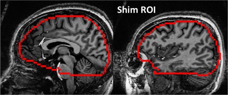
Typical ROI used for B ₀ shimming, shown in two sagittal planes. The ROI encompassed the temporal lobes and covered a longitudinal span of 96 or 99 mm (for (2mm)³ or (3mm)³ isotropic coverage, respectively).

RF Coil and B₁ Shimming

An 8 × 2 (2 rows, 8 coils/row) inductively decoupled elliptical transceiver array was used in parallel transmit mode 26. Each of the eight 1‐kW transmit channels available on this system were split and phase shifted 45°, driving two adjacent within‐row coil pairs. This generated a circularly polarized mode‐like phase distribution, which was optimized by adjusting the amplitude and phase for pairs of coils within different rows. Using a multislice B ₁ mapping acquisition available on the vendor platform, RF shimming was performed as previously described 27. The applied phase for each coil pair was calculated to be constructive over a 60 × 60 mm diameter central ROI spanning seven 3‐mm slices spaced by 12 mm. Using these calculated phases, a least‐squares optimization was performed over the intracranial volume to achieve the target $B_1^{+}$, thus determining the amplitudes for each pair of coils. The achieved $B_1^{+}$ was 460 ± 51 Hz over the entire head at 1140 ± 113 W total applied power.

T₁‐Weighted Anatomical Image

MP2RAGE images 28 were used for anatomical registration using (0.75 mm)³ resolution with TR = 6 s, TE = 3.1 ms, T_I = 0.8/2.7 s, and GRAPPA 3.

(3mm)³ and (2mm)³ Resolution EPI

Single‐shot GE‐EPI were acquired at two spatial resolutions: 3‐mm isotropic (3mm)³: 33 slices, matrix size = 64 × 64, bandwidth per pixel = 20.83 Hz; and 2‐mm isotropic (2mm)³: 48 slices, matrix size = 96 × 96, bandwidth per pixel = 13.88 Hz in n = 6 volunteers. These parameters were selected to keep a fixed echo spacing of 750 μs, thus maintaining equivalent millimeter shifts for the two spatial resolutions.

Other imaging parameters were identical for the two data sets with field of view = 19.2 × 19.2 cm², TR = 3.5 s, TE = 24 ms, phase partial Fourier = 6/8, flip angle = 60°, and 80 repetitions. For ${\mathrm{R}}_2^{*}$ (transverse relaxivity) mapping, multi‐echo gradient‐recalled echo images were acquired using identical dimensions to the GE‐EPI data sets with TR = 3.1 s and TE = 6, 10.39, 16, 21.71, 26.28, 30.85, 35.42, 39.99, 45, and 50 ms for (3mm)³ resolution and TE = 8, 12.57, 17.14, 21.71, 26.28, 30.85, 35.42, 39.99, 50, and 60 ms for (2mm)³ resolution.

Temporal signal‐to‐noise (tSNR) maps were calculated with the exclusion of first five points before reaching a steady state. The BOLD sensitivity was calculated as [echo time] × [signal intensity] 29.

BOLD Breath‐Hold Studies with (2mm)³ Voxel Size

The improvement in GE‐EPI data as a result of higher‐degree shimming was evaluated with functional breath‐hold tests in n = 8 volunteers. For the whole‐brain BOLD signal response, a 21‐s breath‐hold protocol was performed 5 times using a block‐design paradigm (140 s − [21 s (breath hold) – 35 s] × 5). Subjects were asked to exhale before breath‐holding to preclude a biphasic change 30. Each run was acquired with 1^st–2^nd and 1^st–4^th+ degree shimming and signal averaged in randomized order.

The BOLD data were processed using AFNI (http://afni.nimh.nih.gov/afni/), FSL (http://fsl.fmrib.ox.ac.uk/fsl/fslwiki/), and SPM (http://www.fil.ion.ucl.ac.uk/spm/) programs combined with in‐house programs in MATLAB R2013b (MathWorks, Natick, MA USA). Routine image processing included slice‐timing correction, skull stripping, and translational motion correction using FSL and AFNI. The Bolero B ₀ map was used to calculate inhomogeneity‐induced voxel displacements. Following normalization by the mean signal intensity at each voxel, BOLD maps were estimated by linear regression using AFNI (3dDeconvolve), which also included motion parameters. The significance of activation was determined on a pixel‐by‐pixel basis (P < 0.05).

Significance Testing

Significance testing on the change in B ₀ field homogeneity between 1^st–2^nd and 1^st–4^th+ degree shimming was performed in two ways: (i) a paired t‐test was applied to the $\sigma B_0^{\text{Global}}$ measured from each subject (n = 8, Table 1); and (ii) a paired t‐test was used to evaluate the change in the |B ₀| per pixel (including all gray matter, white matter, and CSF pixels.

Table 1.

Comparison of B ₀ Field Homogeneity

Volunteer	${\sigma B}_0^{Global}$		% Difference
	1st–2nd	1st–4th
1	27.66	20.76	24.95
2	31.77	24.09	24.17
3	30.81	24.52	20.42
4	37.37	28.96	22.50
5	29.37	22.18	24.48
6	31.25	23.28	25.50
7	23.98	16.43	31.48
8	25.69	18.79	26.86
Mean	29.74*	22.38*	25.05
SD	4.14	3.83	3.25

*Significantly different, P < 0.01. SD, standard deviation

Significance testing on the echo‐planar images and BOLD data was performed on gray matter pixels binned together according to the difference in their (magnitude) B ₀ offsets achieved with 1^st–2^nd degree shims versus 1^st–4^th+ degree shims (ie, $\Delta \left|B_0\right|=\left|B_0^{1-2}\right|-\left|B_0^{1-4+}\right|$). This binning process generates specific ROIs or parcels that define where the high‐degree shimming achieves its effects (see Fig. 4 for typical distribution of the Δ|B ₀| bins). As binned in 10‐Hz increments, the 10‐Hz bin size corresponds to an approximate 1.5‐mm shift (half of the width of the 3‐mm isotropic image), which is considered to have minimal effect. The magnitude Δ|B ₀| bin of less than −100 Hz represents a large deterioration of field homogeneity with 1^st–4^th+ degree shims, whereas the bin of greater than +100 Hz represents a large improvement. As there is a wide range of Δ|B ₀| values seen at 7 T (although with very few pixels at the greatest extremes), the bin definition for the Δ|B ₀| (either positive or negative) started at a 1% integrated threshold of total pixel numbers. Statistically, for each type of data (BOLD sensitivity, tSNR, or ${\mathrm{R}}_2^{*}$), all pixels from all subjects with a given Δ|B ₀| bin was compared using a paired t‐test between the 1^st–2^nd and 1^st–4^th+ shimming. Each Δ|B ₀| bin was warped into EPI domain using the Bolero‐calculated B ₀ maps to mask the EPI data and generate the binned pixel values of signal intensity and tSNR.

Figure 4.

(a) From n = 8 subjects, the regions of $\Delta \left|B_0\right|=\left|B_0^{1-2}\right|-\left|B_0^{1-4+}\right|$ bins (ie, showing the regions of change in B ₀ shimming) are co‐registered in Talairach space and overlaid on the T₁‐weighted image. As binned in 10‐Hz increments, the positive Δ|B ₀| bins (top) and negative Δ|B ₀| bins (bottom) show regions where 1^st–4^th+ is better or worse than 1^st–2^nd degree shim, respectively. Color bars indicate the 10Hz |B ₀| bins. The volume of positive bins is much larger than negative bins (with most pixels in the negative bins between −10 and −50 Hz). The white line in the sagittal negative bin panel indicates the approximate position of the displayed axial plane. (b) Histogram of gray‐matter pixel numbers over the negative and positive Δ|B ₀| bins (all subjects, calculated in native space), with a magnified view between 0 and 1% of pixel count (bottom).

Similarly, to assess the breath‐hold studies as a function of 1^st–4^th+ versus 1^st–2^nd degree shimming, the BOLD percent change and the number of activated pixels were averaged from all pixels (all subjects) within each ± 10‐Hz Δ|B ₀| bin.

RESULTS

Simulation

Figure 1 shows the B ₀ maps and the simulated signal intensities starting from an anatomical mask, evaluating the ${\mathrm{T}}_2^{*}$ dephasing and pixel shift for 2nd, 4th, 6th, and 10th‐degree whole‐brain shimming. xN indicates the image resolution (ie, summation of N voxels, x1, x8 or x27 representing (1mm)³, (2mm)³, or (3mm)³ sizes. Data from an inferior frontal lobe slice are shown (the red line in upper right in Fig. 1a). As is typical, the $\sigma B_0^{\text{Global}}$ homogeneity improved with increasing degree of applied shimming with 20% improvement between 1^st–2^nd to 1^st–4^th, and 40% with 1^st–6^th. Figure 1b displays magnitude images of the ${\mathrm{T}}_2^{*}$ dephased images at x1, x8 and x27 resolution, with the x8 and x27 images generated by complex summation of the x1 data (by definition there is no signal loss in the x1 images). Figure 1c shows the effect of including pixel shifting. The pixel shifting is greatest in the x1 images and reflects the complex summation of shifted pixels at high resolution, generating decreased and increased pixel intensities, shown here with a dynamic range of 0‐ to 2‐fold in intensity (truncated for better visualization at 2.0; the maximum pixel intensity is approximately 3.0). As shown in Figure 1c, the orbito‐frontal pixels (with positive B ₀ offset, red in the B ₀ map of Fig. 1a) shift posteriorly (thereby decreasing orbito‐frontal signal) to overlap with other pixels over the cavernous sinus. A similar but more subtle effect is seen in the region over the auditory canals, which can generate higher intensity pixels as a result of constructive summation of “collided” pixels caused by anterior and posterior shifts from pixels with B ₀ offsets of opposite sign. At the x8 and x27 resolution, the dephased and shifted images show signal distortion in a combined manner that improves with higher‐degree shimming (right columns of Fig. 1c). At x27, there is a mottled anatomic appearance to the images (bottom panels, Fig. 1b), showing the anatomically linked dephasing effect as a result of the intrinsic susceptibility differences (eg, white‐gray matter) causing a small loss in signal. At all three resolutions, pixel shifting superimposed on complex dephased signal generates both signal gain and loss with the largest x27 pixel size generating lower magnitude signal, with x8 being intermediate to x1 and x27.

Using masks of various brain gray matter parcels (determined by FreeSurfer), the covariance of the signal in each parcel is shown as a function of shim degree (Fig. 1d). As a measure of the signal heterogeneity, the covariance should be 0.0 without any shifting, whereas the complex summation of shifted pixels will result in large covariances (∼1.0). Figure 1e shows the fraction of pixels that move out of its parcel due solely to shifting. In difficult brain regions, more than 50% of pixels do not stay in their original anatomically defined parcel. Although this effect may seem large, it should be recognized that in this simulation, even a small shift (eg, from gray matter into an adjacent white matter or CSF) is counted as a loss (an example of this is shown in the http://onlinelibrary.wiley.com/store/10.1002/mrm.26563/asset/supinfo/mrm26563-sup-0001-suppinfofs1.pdf?v=1&s=96ec8a538e02dfca6e7f84d599434a5a6013b897). In this regard, parcels that have heavily interlaced gray and white matter components may show larger signal loss. Overall, Figures 1d and 1e show that regions with greater susceptibility differences generally experience greater pixel heterogeneity and loss.

Shimming

Over n = 8 subjects, evaluating all intracerebral pixels (extending from the inferior plane of the temporal lobes to the vertex of the brain; see Fig. 2), the use of the high‐degree shims significantly improved the $\sigma B_0^{\text{Global}}$ by 25 ± 3% over the group (P < 0.01; Table 1). To visualize the shimmed B ₀ maps over the n = 8 group, the maps (1^st–2^nd and 1^st–4^th+) were co‐registered into Talairach common brain space, enabling a calculation of the mean and standard deviation maps as shown in Figs. 3a and 3b. However, it should be recognized that the B ₀ distribution will vary depending on both the position and angle of the head within the magnet (in addition to head size and shape); thus, this visual demonstration in Talairach space is solely intended as an approximation (the statistical analysis of all data in this paper is performed in native space). To show B ₀ field detail, the scale of Figure 3a is truncated at ±80 Hz; over n = 8 subjects, the dynamic range in B ₀ values is 423 ± 47 Hz and 390 ± 54 Hz for 1^st–2^nd and 1^st–4^th+ shimming, respectively. Nonetheless, the greatest improvements are in the frontal and temporal lobes.

Figure 3.

Performance of B ₀ shimming. (a) The mean and standard deviation of the B ₀ maps for 1^st–2^nd and 1^st–4^th+ degree shims are displayed in Talairach space (n = 8 subjects). The scale is truncated at ±80 Hz to show detail (note that the dynamic ranges for 1^st–2^nd and 1^st–4^th+ degree shimming are 423 ± 47 Hz and 390 ± 54 Hz, respectively). (b) Histogram analysis for the distribution of B ₀ values for whole brain and gray‐matter area (left: whole brain, right: gray matter) averaged from n = 8 subjects and truncated for display at ±90 Hz with 1^st–4^th+ degree shimming, the center of B ₀ distribution (excluding the 0‐Hz peak) is closer to carrier frequency and narrower than with 1^st–2^nd degree shimming. The peak of 1^st–2^nd degree shimming at the 0‐Hz carrier is marked with blue symbols for visualization from the overlapped peak. It should be noted that the histogram analysis was directly obtained from each subject without transformation into Talairach space.

A histogram analysis of the B ₀ values (Fig. 3c) shows that for both the 1^st–2^nd and 1^st–4^th+ degree shimming there is a large group of pixels at the carrier 0 Hz, although the latter distribution is narrower and closer to the carrier. For both shimming conditions there is also an off‐resonance distribution, with the full width at half maximum (FWHM) and mean offsets being 23.9 ± 4.3 versus 10.6 ± 1.7 Hz (FWHM) and 12.3 ± 4.1 versus 5.8 ± 1.4 Hz (offsets) for the 1^st–2^nd and 1^st–4^th+ degree shimming, respectively. If only gray matter is considered, the FWHM and mean offsets are 28.5 ± 4.4 versus 12.1 ± 1.8 Hz (FWHM) and 11.9 ± 4.4 versus 6.5 ± 1.9 Hz (offsets), respectively, representing 2.4‐ and 1.8‐fold reductions in FWHM and offset.

Figure 4a shows the typical regions of field improvement or deterioration in color‐coded 10‐Hz Δ|B ₀| bins in Talairach space. For each subject, these 10‐Hz bins (each bin separated into gray and white matter pixels) are used in the quantitative analysis throughout the remainder of this report. Considering only gray‐matter pixels, a histogram analysis of each Δ|B ₀| bin (Fig. 4b) shows that 48.6% of pixels are in the center ±10 Hz Δ|B ₀| bins. Excluding these two center bins and integrating over the positive side of the histogram shows that 41.1% of all gray‐matter pixels have decreased frequency offsets (ie, they improved with 1^st–4^th+ degree shimming. Integrating over the negative side shows that 10.2% worsened. Not surprisingly, consistent with the change in $\sigma B_0^{\text{Global}}$ given in Table 1, significance testing on a per‐pixel basis (388,257 gray‐matter pixels, from n = 8 subjects) showed that the reduction in B ₀ offset is highly significant (paired t‐test, P < 10^‐9).

EPI Signal Intensity, tSNR, and ${\mathrm{R}}_2^{*}$

Figure 5 shows (2mm)³ resolution data from a single subject, with representative axial and sagittal slices of the B ₀ maps, original T₁‐weighted image, forward warped T₁‐weighted images (based on the simulation described previously), and raw EPIs. The red contour lines indicate the surface mask (from the original T₁‐weighted images), whereas the blue contour lines indicate the surface mask of the warped T₁‐weighted images. As seen in both the axial and sagittal planes, the forward warped T₁‐weighted images show less destructive interference and signal distortion with 1^st–4^th+ in comparison with 1^st–2^nd shimming. The raw EPIs are similar, showing greater signal intensity in the anterior frontal and inferior orbital regions.

Figure 5.

High‐degree shim effects on EPI data. Axial (left) and sagittal (right) data are shown with matching B ₀ map, T₁‐weighted structural and EPI images. For both axial and sagittal data: (a) the original T₁‐weighted structural image with a red contour line showing the brain edge; (b) the 1^st–2^nd shimmed B ₀ map, forward‐warped T₁‐weighted image with original red edge contour and blue contour showing the edge of the warped T₁ image (using the displayed B ₀ map), and the original (2mm)³ EPI data with superimposed contour lines; (c) the 1^st–4^th+ shimmed B ₀ map, forward‐warped T₁‐weighted image with original red edge contour and blue contour showing the edge of the 1^st–4^th+ warped T₁ image, and the (2mm)³ EPI data with superimposed contour lines. The unevenness of the blue contour edge reflects the high variability of the shifted pixels, particularly seen in the inferior frontal and occipital region.

Figure 6 shows the (2mm)³ and (3mm)³ tSNR and ${\mathrm{R}}_2^{*}$ maps from the same subject as Figure 5. To show the pertinent signal variation, both sets of images are scaled to a truncated range as indicated. The tSNR at (3mm)³ is 24% larger than the (2mm)³. Both the tSNR and ${\mathrm{R}}_2^{*}$ show small but consistent differences between the 1^st–2^nd and 1^st–4^th+ shimmed data, with the greatest differences seen in high‐susceptibility regions.

Figure 6.

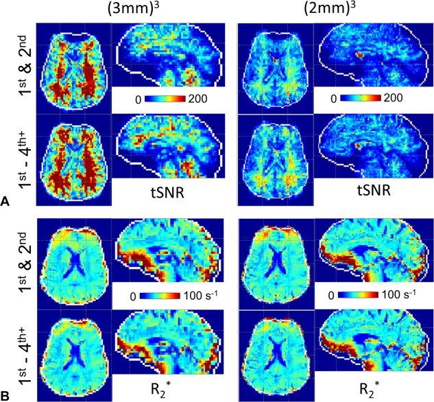
High‐degree shim effects on tSNR and ${\mathrm{R}}_2^{*}$ from a single subject. (a) Higher tSNR is observed with (3mm)³ as compared with (2mm)³ resolution as expected, and shows increases with 1^st–4^th +degree shimming. (b) The ${\mathrm{R}}_2^{*}$ values are slightly improved with 1^st–4^th +degree shimming. Color bars indicate tSNR and ${\mathrm{R}}_2^{*}$ values.

The gray‐matter statistics from several performance metrics, BOLD sensitivity, ${\mathrm{R}}_2^{*}$, and tSNR from (2mm)³ studies (n = 6) are assessed as a function of Δ|B ₀| in Figure 7. For statistical analysis, the highest (either positive or negative) Δ|B ₀| bin integrates all of the higher Δ|B ₀| bins to achieve at least a 1% threshold pixel count. Because the high‐degree shim insert generally improved the B ₀ offset, the 1% threshold results in the most positive bin starting at +100 Hz, whereas the most negative bin starts at $-$ 70 Hz. With significance testing (paired t‐tests, P < 0.05) performed on a per‐pixel basis in each bin, the changes in BOLD sensitivity (red circles) and ${\mathrm{R}}_2^{*}$ (green squares) were significant over many of both the positive and negative bins. Although the ${\mathrm{R}}_2^{*}$ values in the highest positive Δ|B ₀| bins (>80 Hz) appear to worsen, it is likely that the TEs used in this study were not short enough to accurately measure very high ${\mathrm{R}}_2^{*}$ values (>100 s^‐1), which combined with the small number of pixels, compromises the accuracy of these ${\mathrm{R}}_2^{*}$ measurements. Notably, however, the percentage change in tSNR is relatively constant across the Δ|B ₀| bins. This likely reflects a combined effect of shift‐induced complex signal interference (constructive or destructive) and local B ₀ inhomogeneity–induced dephasing. White‐matter pixels (characterized by higher tSNR) that shift over gray‐matter pixels can increase tSNR, thereby appearing to improve tSNR in negative Δ|B ₀| bins in spite of increased dephasing losses. In comparison, in the positive Δ|B ₀| bins, the improved tSNR argues that the improved dephasing contributes more than the decrease of white‐matter overlap. Thus, for evaluation of B ₀ homogeneity, tSNR can be complicated, reflecting $\overline{SI}/\sigma \left(SI\right)$.

Figure 7.

Evaluation of EPI signal metrics in (2mm)³ gray‐matter EPI pixels over $\Delta \left|B_0\right| =\left|B_0^{1-2}\right|-\left|B_0^{1-4+}\right|$ bins for n = 6 subjects combined. The highest (either positive or negative) Δ|B ₀| bin integrates all of the higher Δ|B ₀| bins so as to start with a 1% threshold pixel count. The BOLD sensitivity, tSNR, and ${\mathrm{R}}_2^{*}$ increased in the positive Δ|B ₀| bins, whereas they decreased in the negative Δ|B ₀| bins. Because most of the bins were significantly different (P < 0.05) between the 1^st–2^nd and 1^st–4^th+ shims, the “x” indicates the nonsignificant bins.

BOLD Study with (2mm)³ Voxel Size

Finally, it is important to establish whether the improvements in B ₀ ultimately result in improved BOLD activation. Grouped data from n = 8 breath‐hold studies are shown in Figure 8a as a function of Δ|B ₀| bin. Similar to Figure 7, the bins are analyzed on a per‐pixel basis using paired t‐tests. Over many of both the positive and negative bins, the BOLD percentage signal change is significant, increasing in the positive bins and decreasing in the negative bins. More commonly seen across both positive and negative bins, however, is the change in numbers of activated pixels. Over the n = 8 volunteers, Figure 8a shows that the high‐degree shimming significantly increased the number of activated pixels in the positive Δ|B ₀| bins, whereas they decreased in the negative bins (note that for the activated pixel numbers (green symbols), all bins were significantly different between 1^st–2^nd and 1^st–4^th+ shimming). Regionally, as shown in Talairach space, Figure 8b shows the locations and fractional change in activated pixels. For example, in the Δ|B ₀| bins of + 70 Hz (2625 total gray‐matter pixels) and +60 Hz (4631 total gray‐matter pixels), there is an increase of 24 and 29%, respectively, in the number of activated pixels, whereas there is a significant decline in activated pixels in the negative Δ|B ₀| bins (eg, in the −70 Hz (610 total gray‐matter pixels) and −60 Hz (1071 total gray‐matter pixels) bins there is a decrease of −32 and −14%, respectively). The importance in pixel numbers between the positive and negative bins becomes more evident when considering the ratio of gained (activated pixel counts summed over positive bins: 1^st–4^th+ minus 1^st–2^nd) to lost (activated pixel counts summed over negative bins, 1^st–2^nd minus 1^st–4^th+). When excluding the center two Δ|B ₀| bins, this ratio is 7.9 (ie, for every 1 pixel lost, there are 7.9 pixels gained). Averaging over the entire head, given that most pixels stay in the center Δ|B ₀| bins, the high‐degree shim results in a 4.3% increase in activated pixel numbers. Finally, as an example, Figure 9 displays the activation maps from a single subject.

Figure 8.

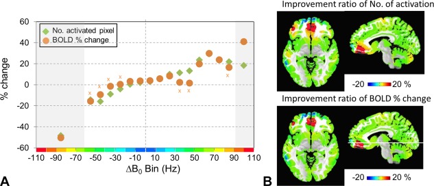
Evaluation of functional activation over the Δ|B ₀| bins (see Fig. 4 for definition of bins). (a) The number of activated pixels and BOLD percentage change increased in the positive Δ|B ₀| bins, particularly above + 40 Hz. From the negative Δ|B ₀| bins, the number of activated pixels and BOLD percentage change decreased. For all bins, the activated pixel numbers (green) were significantly different between 1^st–2^nd and 1^st–4^th+ shims. For most of the bins, the BOLD percentage signal change (orange) was significantly different (P < 0.05) between the 1^st–2^nd and 1^st–4^th +shims; the bins that were nonsignificant (BOLD percentage signal change) are marked by “x.” (b) The regional location of each Δ|B ₀| bin (corresponding to that shown in Fig. 3) is shown in color according to the fractional change in either activated pixel number or BOLD percentage signal change as defined from (a).

Figure 9.

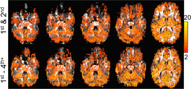
BOLD activation maps are shown from a single subject: maps from 1^st–2^nd (top) and 1^st–4^th+ shimming (bottom) are overlaid on the forward‐warped T₁‐weighted images (using the Bolero B ₀ maps). The t‐value is shown in the color scale.

DISCUSSION

Improved B ₀ Field Homogeneity: In Simulation

For 7T EPI, we simulated the pixel‐shifting effect in EPI to determine the final location of pixels located in regions with high B ₀ inhomogeneity. It should be noted (as stated in the “Methods” section) that the signal intensities seen in Figure 1 should not be regarded as a strict match to the EPI acquisition. Nonetheless, the shift simulation shows that there is good agreement between the resulting maps and the EPI with 1^st–2^nd and 1^st–4^th+ degree shims (Fig. 5), indicating the accuracy of the B ₀ field maps. As shown in Figure 1, the shifting of complex signal results in constructive and destructive interference. It should be noted that although Figure 1c shows an apparent maximum signal intensity of 3.0 in high “collision” areas, the actual number of overlapping pixels is much higher (eg, in the location of the apparent 3.0 signal intensity, 14 pixels are overlapped). Furthermore, as identified in Figure 1e, many pixels may be shifting in and out of the anatomical parcel of interest, resulting in a large apparent loss of pixels in any given parcel. As shown in http://onlinelibrary.wiley.com/store/10.1002/mrm.26563/asset/supinfo/mrm26563-sup-0001-suppinfofs1.pdf?v=1&s=96ec8a538e02dfca6e7f84d599434a5a6013b897, the amount of shift that causes this does not have to be large, given the exclusion of pixels after they have moved into adjacent white‐matter regions. In addition, simple backward warping of these overlapped pixels does not restore the proper signal, given the complex interference occurring in all pixels.

Improved B ₀ Field Homogeneity: Experimental

Experimentally, high‐degree shimming improves the overall B ₀ field homogeneity by generally reducing the inhomogeneity of poorly shimmed high‐susceptibility regions while retaining the homogeneity of well‐shimmed regions. As shown in Figure 3, 1^st–4^th+ shimming increases the number pixels at the center of the B ₀ distribution (0 Hz) while narrowing the distribution of the remainder. As a function of the Δ|B ₀| bin, 48.6% of all gray‐matter pixels are retained within the central two Δ|B ₀| bins, while 41.1% showed improvement, ΔB ₀ > 10 Hz, and 10.2% worsened (Fig. 4b). When including white‐matter pixels, 50.7% were maintained, 40.6% improved, whereas 8.7% worsened.

The ability to improve the homogeneity from high‐susceptibility regions while retaining most of the existing regions is enabled by the shim insert's greater spatial complexity of B ₀ relative to 1^st–2^nd degree shims. However, it should be noted that the large target shim volume includes regions where the spatial inhomogeneities exceed 4^th+ degree and cannot be completely compensated for simultaneously. In these regions, the homogeneity can be further optimized with restricted regional shimming and theoretically by use of even higher degree shim terms (eg, up to 7th degree 25).

Simultaneous Whole‐Brain B ₀ Homogeneity for EPI and BOLD Activation

The wide‐spread use of SMS EPI methods makes simultaneous whole‐brain shimming an important target. Most reports on this are based on spherical harmonic shimming (given that 1^st–2^nd degree spherical harmonic shims are the most common hardware on human MRI systems), although there has been variability in the results. At 3 T, Wilson 31 reported $\sigma B_0^{\text{Global}}$ with 1^st–2^nd degree shims at 24 Hz (0.20 ppm), whereas Stockmann 19 reported 31.8 Hz. At 7 T, these values would scale to 58 and 77 Hz, respectively. However, at 7 T, Juchem 17 reported a $\sigma B_0^{\text{Global}}$ of 32.3 ± 5.5 Hz using 1^st–3^rd degree shimming. The present experimental data (similar to Kim 32) reports 29.7 ± 4.1 Hz and 22.4 ± 3.8 Hz for 1^st–2^nd and 1^st–4^th+, respectively (Table 1). Overall, it is possible that the observed variability is the result of subject variation (eg, head tilt and shape), user‐defined regions for shimming, or other methodological differences.

Nonetheless, demonstration of increased BOLD activation is clearly a target for all of these methods. For example, Hsu and Glover 9 used a direct‐current mouth insert to gain 26% in activated pixels in the inferior frontal lobe at 1.5 T (3.75 × 3.75 × 5 mm³ pixel size, spiral trajectory). This improvement is similar to the present data with a 24 to 29% increase in the inferior frontal region where the Δ|B ₀| bins show a large improvement (bins > +50 Hz, Figs. 4a and 9). In regions of Δ|B ₀| deterioration found in the frontal pole and a portion of the lateral temporal lobe, the fractional decline in activated pixels is similar, $-$32.2 to −16%, although the number of pixels in these negative bins (−50 to −70 Hz) is 4.6‐fold smaller than the equivalent positive bins. Summing over the entire brain, the large number of relatively unchanged pixels dominates, resulting in a 4.3% increase in total activated pixels.

CONCLUSIONS

The work of Speck 33 finding the highest BOLD sensitivity at 1.4 to 2‐mm isotropic resolution, together with the enhanced SNR at 7 T makes high‐resolution BOLD imaging a key target. However, with limited gradient performance, the higher resolution requires longer single‐shot encoding times, which is already restricted because of the relatively short optimal TE at 7 T ( ${\mathrm{T}}_2^{*}$ of gray matter being ∼25 ms 34). Although parallel imaging techniques such as GRAPPA can increase spatial resolution without causing distortion, this also reduces SNR. Alternatively, multi‐echo EPI can also be considered to improve BOLD studies 35, 36, although at a cost of lower spatial resolution or increased TRs to accommodate the multiple echo measurements. As an independent means of improving field homogeneity, high‐degree shimming does not interact with other imaging parameters and is compatible with whole‐brain coverage necessary for simultaneous multislice methods. Comparing 1^st–2^nd and 1^st–4^th+ shimming, the Δ|B ₀| changes vary spatially over the brain with most of the brain either maintaining or increasing signal intensity and activation. Focusing on the pixels that substantially change (either improved or worsened, outside of the two center Δ|B ₀| bins) with the 1^st–4^th+ shimming, for each activated pixel that is lost, there are 7.9 activated pixels gained. The largest regions of activation increase are seen in the inferior frontal region, whereas the largest regions of activation decrease are in the middle temporal lobe. Overall, there is a 4.3% increase in total activated pixels.

Supporting information

Fig. S1. Simulation of pixel shift caused by B ₀ inhomogeneity. (Left) The B ₀ map is overlaid on the segmented white‐matter mask. (Middle) The gray matter orbitofrontal region is shown as a red ROI superimposed on the white matter mask. (Right) With shifting, gray‐matter orbitofrontal pixels (red) move into adjacent white matter, gray matter, and CSF regions.

REFERENCES

- 1. Hutton C, Bork A, Josephs O, Deichmann R, Ashburner J, Turner R. Image distortion correction in fMRI: a quantitative evaluation. NeuroImage 2002;16:217–240. [DOI] [PubMed] [Google Scholar]
- 2. Jezzard P, Balaban RS. Correction for geometric distortion in echo planar images from B0 field variations. Magn Reson Med 1995;34:65–73. [DOI] [PubMed] [Google Scholar]
- 3. Constable RT, Spencer DD. Composite image formation in z‐shimmed functional MR imaging. Magn Reson Med 1999;42:110–117. [DOI] [PubMed] [Google Scholar]
- 4. Frahm J, Merboldt KD, Hanicke W. Direct FLASH MR imaging of magnetic field inhomogeneities by gradient compensation. Magn Reson Med 1988;6:474–480. [DOI] [PubMed] [Google Scholar]
- 5. Glover GH. 3D z‐shim method for reduction of susceptibility effects in BOLD fMRI. Magn Reson Med 1999;42:290–299. [DOI] [PubMed] [Google Scholar]
- 6. Young IR, Cox IJ, Bryant DJ, Bydder GM. The benefits of increasing spatial resolution as a means of reducing artifacts due to field inhomogeneities. Magn Reson Imaging 1988;6:585–590. [DOI] [PubMed] [Google Scholar]
- 7. Cho ZH, Ro YM. Reduction of susceptibility artifact in gradient‐echo imaging. Magn Reson Med 1992;23:193–200. [DOI] [PubMed] [Google Scholar]
- 8. Stenger VA, Boada FE, Noll DC. Three‐dimensional tailored RF pulses for the reduction of susceptibility artifacts in T2* weighted functional MRI. Magn Reson Med 2000;44:525–531. [DOI] [PMC free article] [PubMed] [Google Scholar]
- 9. Hsu JJ, Glover GH. Mitigation of susceptibility‐induced signal loss in neuroimaging using localized shim coils. Magn Reson Med 2005;53:243–248. [DOI] [PubMed] [Google Scholar]
- 10. Wilson JL, Jezzard P. Utilization of an intra‐oral diamagnetic passive shim in functional MRI of the inferior frontal cortex. Magn Reson Med 2003;50:1089–1094. [DOI] [PubMed] [Google Scholar]
- 11. Osterbauer RA, Wilson JL, Calvert GA, Jezzard P. Physical and physiological consequences of passive intra‐oral shimming. NeuroImage 2006;29:245–253. [DOI] [PubMed] [Google Scholar]
- 12. Koch KM, Rothman DL, de Graaf RA. Optimization of static magnetic field homogeneity in the human and animal brain in vivo. Prog Nucl Magn Reson Spectrosc 2009;54:69–96. [DOI] [PMC free article] [PubMed] [Google Scholar]
- 13. Sengupta S, Welch EB, Zhao Y, Foxall D, Starewicz P, Anderson AW, Gore JC, Avison MJ. Dynamic B0 shimming at 7 T. Magn Reson Imaging 2011;29:483–496. [DOI] [PMC free article] [PubMed] [Google Scholar]
- 14. Morrell G, Spielman D. Dynamic shimming for multi‐slice magnetic resonance imaging. Magn Reson Med 1997;38:477–483. [DOI] [PubMed] [Google Scholar]
- 15. Blamire AM, Rothman DL, Nixon T. Dynamic shim updating: a new approach towards optimized whole brain shimming. Magn Reson Med 1996;36:159–165. [DOI] [PubMed] [Google Scholar]
- 16. de Graaf RA, Brown PB, McIntyre S, Rothman DL, Nixon TW. Dynamic shim updating (DSU) for multislice signal acquisition. Magn Reson Med 2003;49:409–416. [DOI] [PubMed] [Google Scholar]
- 17. Juchem C, Nixon TW, Diduch P, Rothman DL, Starewicz P, de Graaf RA. Dynamic shimming of the human brain at 7 Tesla. Conc Magn Reson B Magn Reson Eng 2010;37B:116–128. [DOI] [PMC free article] [PubMed] [Google Scholar]
- 18. Han H, Song AW, Truong TK. Integrated parallel reception, excitation, and shimming (iPRES). Magn Reson Med 2013;70:241–247. [DOI] [PMC free article] [PubMed] [Google Scholar]
- 19. Stockmann JP, Witzel T, Keil B, Polimeni JR, Mareyam A, LaPierre C, Setsompop K, Wald LL. A 32‐channel combined RF and B0 shim array for 3T brain imaging. Magn Reson Med 2016;75:441–451. [DOI] [PMC free article] [PubMed] [Google Scholar]
- 20. Juchem C, Umesh Rudrapatna S, Nixon TW, de Graaf RA. Dynamic multi‐coil technique (DYNAMITE) shimming for echo‐planar imaging of the human brain at 7 Tesla. NeuroImage 2015;105:462–472. [DOI] [PMC free article] [PubMed] [Google Scholar]
- 21. Moeller S, Yacoub E, Olman CA, Auerbach E, Strupp J, Harel N, Ugurbil K. Multiband multislice GE‐EPI at 7 tesla, with 16‐fold acceleration using partial parallel imaging with application to high spatial and temporal whole‐brain fMRI. Magn Reson Med 2010;63:1144–1153. [DOI] [PMC free article] [PubMed] [Google Scholar]
- 22. Abramowitz M, Stegun I. Handbook of Mathematical Functions. Mineola, NY: Dover Publications; 1965. p 1046. [Google Scholar]
- 23. Hillenbrand D, Lo K, Punchard W, Reese T, Starewicz P. High order MR shimming: a simulation study of the effectiveness of competing methods, using an established susceptibility model of the human head. Appl Magn Reson 2005:29:39–64. [Google Scholar]
- 24. Hetherington HP, Chu WJ, Gonen O, Pan JW. Robust fully automated shimming of the human brain for high‐field 1H spectroscopic imaging. Magn Reson Med 2006;56:26–33. [DOI] [PubMed] [Google Scholar]
- 25. Pan JW, Lo KM, Hetherington HP. Role of very high order and degree B0 shimming for spectroscopic imaging of the human brain at 7 tesla. Magn Reson Med 2012;68:1007–1017. [DOI] [PMC free article] [PubMed] [Google Scholar]
- 26. Avdievich NI. Transceiver‐phased arrays for human brain studies at 7 T. Appl Magn Reson 2011;41:483–506. [DOI] [PMC free article] [PubMed] [Google Scholar]
- 27. Hetherington HP, Avdievich NI, Kuznetsov AM, Pan JW. RF shimming for spectroscopic localization in the human brain at 7 T. Magn Reson Med 2010;63:9–19. [DOI] [PMC free article] [PubMed] [Google Scholar]
- 28. Marques JP, Kober T, Krueger G, van der Zwaag W, Van de Moortele PF, Gruetter R. MP2RAGE, a self bias‐field corrected sequence for improved segmentation and T1‐mapping at high field. NeuroImage 2010;49:1271–1281. [DOI] [PubMed] [Google Scholar]
- 29. Deichmann R, Josephs O, Hutton C, Corfield DR, Turner R. Compensation of susceptibility‐induced BOLD sensitivity losses in echo‐planar fMRI imaging. NeuroImage 2002;15:120–135. [DOI] [PubMed] [Google Scholar]
- 30. Li TQ, Kastrup A, Takahashi AM, Moseley ME. Functional MRI of human brain during breath holding by BOLD and FAIR techniques. NeuroImage 1999;9:243–249. [DOI] [PubMed] [Google Scholar]
- 31. Wilson JL, Jenkinson M, Jezzard P. Optimization of static field homogeneity in human brain using diamagnetic passive shims. Magn Reson Med 2002;48:906–914. [DOI] [PubMed] [Google Scholar]
- 32. Kim T, Lee Y, Zhao T, Starewicz P, Hetherington H, Pan J. Reducing susceptibility‐induced signal loss in echo planar imaging using a shim insert coil at 7T: implication for BOLD fMRI. In Proceedings of the 22nd Annual Meeting of ISMRM, Milan, Italy; 2014. p. 863.
- 33. Speck O, Stadler J, Zaitsev M. High resolution single‐shot EPI at 7T. Magma 2008;21:73–86. [DOI] [PubMed] [Google Scholar]
- 34. Yacoub E, Shmuel A, Pfeuffer J, Van De Moortele PF, Adriany G, Andersen P, Vaughan JT, Merkle H, Ugurbil K, Hu X. Imaging brain function in humans at 7 Tesla. Magn Reson Med 2001;45:588–594. [DOI] [PubMed] [Google Scholar]
- 35. Poser BA, Versluis MJ, Hoogduin JM, Norris DG. BOLD contrast sensitivity enhancement and artifact reduction with multiecho EPI: parallel‐acquired inhomogeneity‐desensitized fMRI. Magn Reson Med 2006;55:1227–1235. [DOI] [PubMed] [Google Scholar]
- 36. Posse S, Wiese S, Gembris D, Mathiak K, Kessler C, Grosse‐Ruyken ML, Elghahwagi B, Richards T, Dager SR, Kiselev VG. Enhancement of BOLD‐contrast sensitivity by single‐shot multi‐echo functional MR imaging. Magn Reson Med 1999;42:87–97. [DOI] [PubMed] [Google Scholar]
Associated Data
This section collects any data citations, data availability statements, or supplementary materials included in this article.
Supplementary Materials
Fig. S1. Simulation of pixel shift caused by B 0 inhomogeneity. (Left) The B 0 map is overlaid on the segmented white‐matter mask. (Middle) The gray matter orbitofrontal region is shown as a red ROI superimposed on the white matter mask. (Right) With shifting, gray‐matter orbitofrontal pixels (red) move into adjacent white matter, gray matter, and CSF regions.