A spatial frequency spectral peakedness model predicts discrimination performance of regularity in dot patterns

Abstract

Subjective assessments of spatial regularity are common in everyday life and also in science, for example in developmental biology. It has recently been shown that regularity is an adaptable visual dimension. It was proposed that regularity is coded via the peakedness of the distribution of neural responses across receptive field size. Here, we test this proposal for jittered square lattices of dots. We examine whether discriminability correlates with a simple peakedness measure across different presentation conditions (dot number, size, and average spacing). Using a filter-rectify-filter model, we determined responses across scale. Consistently, two peaks are present: a lower frequency peak corresponding to the dot spacing of the regular pattern and a higher frequency peak corresponding to the pattern element (dot). We define the “peakedness” of a particular presentation condition as the relative heights of these two peaks for a perfectly regular pattern constructed using the corresponding dot size, number and spacing. We conducted two psychophysical experiments in which observers judged relative regularity in a 2-alternative forced-choice task. In the first experiment we used a single reference pattern of intermediate regularity and, in the second, Thurstonian scaling of patterns covering the entire range of regularity. In both experiments discriminability was highly correlated with peakedness for a wide range of presentation conditions. This supports the hypothesis that regularity is coded via peakedness of the distribution of responses across scale.

1 Introduction

Regular spatial patterns appear in natural and artificial systems at a wide range of scales. Although not always defined, regularity can be regarded as a simple law that governs the appearance of an image. There exist distinct types of regularity and these may depend on the specific features of the image. For example, we frequently encounter patterns with repeating elements placed at equal spacings. This type of pattern is defined by the set of element locations (called the point pattern), and the form of the individual elements placed at each point (e.g., dots, as used here). Such an arrangement can be described by a straightforward law of periodicity according to which, neglecting edge effects, an image, I, appears identical to itself, when it is translated by an integer number, m, of a quantized step, d⃗, in one or more directions (i.e., I(x⃗ + md⃗) = I(x⃗)). Similar invariance laws can also describe reflection or rotational symmetries and are well studied (Miller, 1972; O’Keeffe & Hyde, 1996; Griffin, 2009). Vision strongly engages with regularity even when the underlying law is not identified or cognitively accessible as, for example, in Glass patterns (Glass, 1969) or in patterns with self-similarity at multiple scales. Specific types of symmetry have been appreciated and used historically in architecture and arts long before their explicit mathematical formulation was derived.

Regularities may interact synergistically (Wagemans, Wichmann & Op de Beeck, 2005) and in a generally unpredictable fashion. For example, when the horizontal distance between dots in a square lattice decreases, this can give rise to a new percept: the appearance of notional vertical lines (Wagemans, Eycken, Claessens & Kubovy, 1999). Regularity can cause pop-out effects and can be considered a type of Gestalt (Koffka, 1935; Ouhnana, Bell, Solomon & Kingdom, 2013). Attneave (1954) considered the ability of the visual system to detect regularity as a mechanism of the perceptual machinery to reduce redundancy by compressing information and thus increase coding efficiency. In nature, perfect regularity is rare. The visual system most often deals with partial regularity, i.e., some amount of departure from perfect regularity. In textures, the degree of regularity is a cue for texture discrimination and segmentation (Bonneh, Reisfeld & Yeshurun, 1994; Vancleef, Putzeys, Gheorghiu, Sassi, Machilsen & Wagemans, 2013). Regularity also interacts with other perceptual dimensions, e.g., numerosity (Whalen, Gallistel & Gelman, 1999) and needs to be controlled in psychophysical experiments (Allïk & Tuulmets, 1991; Bertamini, Zito, Scott-Samuel & Hulleman, 2016; Burgess & Barlow, 1983; Cousins & Ginsburg, 1983; Ginsburg, 1976, 1980; Ginsburg & Goldstein, 1987). Similarly, in contour-integration tasks, stimuli of intermediate regularity must be used to avoid density cues (Demeyer & Machilsen, 2012; Machilsen, Wagemans & Demeyer, 2015).

Perception of partial regularity is useful for scientific analysis. Researchers very often rely on vision to assess the degree of organization in patterns encountered in the study of evolving systems. Partial regularity is essential in natural sciences. In biological organisms, high regularity is advantageous as it affects efficiency (e.g., in the eye it allows for a high density of receptors at the fovea), while lack of regularity manifests as disease (e.g., cancer) and compromised homeostasis. In some processes, however, what is crucial is the balance between perfect and partial regularity. For example, during development, dynamic noise keeps tissue in a state of intermediate regularity, protecting cell proliferation by maintaining a dynamic equilibrium between newly generated cells with division processes and cell death. In this way, biological functions are able to adjust to changes and so exhibit robustness across different developmental conditions (Cohen, Baum & Miodownik, 2011; Cohen, Georgiou, Stevenson, Miodownik & Baum, 2010; Marinari, Mehonic, Curran, Gale, Duke & Baum, 2012). Interestingly, despite its importance, there is no unified framework for estimation of the degree of regularity. Rather, there are a variety of isolated approaches (e.g., Cliffe & Goodwin, 2013; Dunleavy, Wiesner & Royall, 2012; Jiao, Lau, Hatzikirou, Meyer-Hermann, Corbo & Torquato, 2014; Sausset & Levine, 2011; Steinhardt, Nelson & Ronchetti, 1983; Truskett, Torquato & Debenedetti, 2000). Occasionally, researchers are hesitant to trust measures they use, as they report an obvious disagreement between the measure and what they perceive visually when examining the organization of a system (Cook, 2004). Humans are particularly consistent in their judgments of regularity even for diverse sets of stimuli (Protonotarios, Baum, Johnston, Hunter & Griffin, 2014; Protonotarios, Johnston & Griffin, 2016), and since these judgments have an interval-scale structure (Stevens, 1946), they can be used as a basis for quantification. By analyzing the process of pattern formation in the developing Drosophila epithelium, it has been demonstrated that an objective surrogate of perceived regularity can be used for scientific analysis (Protonotarios, Baum, Johnston, Hunter & Griffin, 2014).

Regularity is thus an important aspect of stimuli for the visual system. However, little is known about how it is encoded in the brain. Ouhnana et al. (2013) showed that regularity is an adaptable visual dimension, and proposed that it is coded via the peakedness of the distribution of neural responses across receptive-field size. They used patterns consisting of luminance-defined (Gaussian blobs), and contrast-defined (difference of Gaussians and random binary patterns) elements arranged on a square grid, and they varied the degree of regularity by randomly jittering their position. It was found that a test pattern appears less regular after adaptation to a pattern of similar or higher degree of regularity. The strength of this uni-directional aftereffect was dependent on the degree of regularity of the adapting pattern, with higher regularity causing a stronger effect. Based on the observation that the amplitude of the Fourier transformation of a regular pattern is also regular, they suggested that regularity information is carried mainly by the amplitude spectrum and not the phase. They proposed that regularity is coded via the pattern of response amplitudes of visual filters of varying receptive-field size and that adaptation alters this pattern of responses.

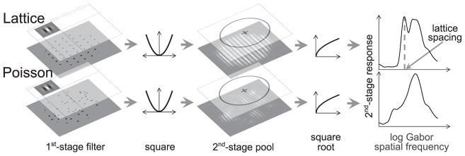
To illustrate the point, they simulated a simple filter-rectify-filter model of neural responses (Graham, 2011) and examined the distribution of responses across scale for a perfectly regular and a random-dot pattern. The sequence of processing stages is illustrated in Figure 1. First, a bank of bandpass filters of varying size is applied to the image. Here, the receptive fields are vertical Gabors:

$$F(x,y)=\mathit{exp}\left(-\frac{x^2+y^2}{2{\sigma }^2}\right)\mathit{cos}(2\pi fx),$$ (1)

with the standard deviation of the Gaussian envelope, σ, varying to cover a range of spatial scales. σ covaried with spatial frequency, f, according to:

$$\sigma =\frac{1}{\pi f}\sqrt{\frac{ln2}{2}}\frac{2^b+1}{2^b-1}$$ (2)

to maintain a constant full-width, half-height spatial frequency bandwidth, b (in octaves). The Gabor filter is normalized by a factor of σ² to keep energy sensitivity constant across scale. The responses of the first-stage filter are then rectified by squaring and a second-stage low-pass filter sums the output over a large region and takes the square root. Figure 1 illustrates the output of the filter-rectify-filter cascade across scale for a regular and an irregular dot pattern. In the spectrum of the regular pattern two predominant peaks can be seen. The first appears at lower spatial frequency and coincides with the lattice spacing, while a second broader peak at higher frequency corresponds to the pattern element (dot) size. The first peak is absent in the irregular pattern. Although this analysis is applied to patterns of luminance-defined elements, it can be easily generalized to contrast-defined elements by the introduction of an additional intermediate stage of bandpass filters and non-linearity (Ouhnana et al., 2013). Ouhnana and colleagues (2013) suggested that regularity is coded via some measure of peakedness of this distribution.

Figure 1.

Demonstration of the filter-rectify-filter process for two dot patterns. The top row demonstrates the process for a perfectly regular pattern and the bottom row for a Poisson pattern. The dot pattern was convolved with a series of Gabor filters of varying spatial scale. The outputs were squared and pooled across a fixed circular area and then a final square root nonlinearity was applied. Comparing the two spectra, one can see the narrow peak that corresponds to the lattice spacing in the upper-right graph; this peak is absent for the Poisson pattern.

We can use data from previous work to verify that this is a reasonable assumption. We examined the perception of regularity for dot patterns that were based on a square lattice (Protonotarios et al., 2016). Regularity was varied using positional jitter. We used patterns that covered the whole range of regularity, from a perfect lattice to total randomness (a Poisson pattern). Figure 2 shows five example patterns. We used the more general term order to describe the degree of organization of the dot patterns. However, for this simple class of stimuli based on a reference pattern (a square grid), with deviation from regularity controlled by a single variable, we consider the terms order and regularity to be synonymous. We used Thurstonian scaling (Thurstone, 1927) on judgments of relative regularity between pairs of patterns and showed that humans can distinguish up to 16.5 just-noticeable-difference (JND) levels between total randomness and perfect regularity.

Figure 2.

Dot patterns exhibiting different levels of regularity. All patterns were based on the same square lattice of points and regularity was controlled by the amount of positional jitter.

Using the derived perceptual regularity values from the scaling procedure we can test whether these are in agreement with the height of the peak that corresponds to the lattice spacing in the spectrum of responses across scale. Figure 3 shows that peak height correlates exceptionally well with fitted regularity value (Pearson correlation coefficient ρ = 0.99). Although this appears to be a very strong validation of the hypothesis that regularity is coded via this simple measure of peakedness, an examination of alternative quantifications gave comparable correlation values. For example, geometrical measures based on the coordinates of the centers of the dots such as, for example, the square root of the variance of the nearest-neighbor distances, also correlates well with the fitted regularity values (ρ = −0.98). Even a simplistic measure—the single shortest pairwise distance between any points in the pattern — correlates highly (ρ = 0.96), even though it is clear that this measure cannot possibly estimate overall regularity in general. Since a variety of quantifications based on point coordinates or Gabor filter responses all correlate comparably well with perceived regularity for such a simple class of stimuli, it is important to examine a broader class of stimuli.

Figure 3.

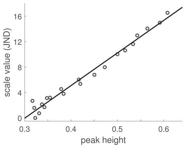
Discrimination scale values from Thurstonian scaling vs. height of the peak at the spatial frequency corresponding to the lattice periodicity in the distribution of responses across scale. Data from Protonotarios and colleagues (2016).

Here, rather than using a more diverse stimulus set, which could introduce additional complexity, we consider an alternative approach for testing the hypothesis about regularity coding suggested by Ouhnana and colleagues (2013). The idea is illustrated in Figure 4. Although point patterns are abstract mathematical entities, concrete choices have to be made about how they are displayed for human observers. A finite number of points have to be depicted in a limited area with the use of small visual elements that carry little information over and above their location. We chose to use dots for the depiction of point patterns as these are the simplest elements with circular symmetry and dot patterns are commonly used for analysis in a variety of scientific fields where subjective assessments of regularity are employed. However, even for a dot pattern based on the same set of xy coordinates, distinct presentation conditions can be chosen by varying dot size and average dot spacing. These give rise to unequal distributions of responses across scale. Figure 4 shows response distributions for a perfect lattice and a random Poisson dot arrangement for two presentation conditions differing in dot size. The curves have been scaled so that the broad peak at high spatial frequency that corresponds to the dot has a y-value of 1. Considering the distribution of responses of the perfect lattice, we define the peakedness associated with a presentation condition as the height on this rescaled spectrum of the narrow peak that corresponds to the spacing of the regular grid. If we assume a single neural read-out mechanism for the peak value common for all conditions, and consider the fact that the peak is absent for the random arrangement of dots and maximum for the regular grid, we predict that the conditions associated with higher peakedness values will result in better discrimination performance. Because we use relative responses for this measure, this implies that performance should be independent of contrast (as long as the signal-to-noise ratio is sufficiently high) and dot number. The latter prediction assumes that the second stage of the filter process pools over a sufficiently large area, so that dot number should not affect discrimination performance. We predict that a condition with larger peakedness (by which we mean the range from fully random to fully regular) will result in better discrimination performance between different amounts of jitter and a larger number of JNDs across the full range of regularity. We test these predictions in the two experiments reported below.

Figure 4.

Definition of peakedness and comparison of corresponding values for patterns that differ in dot size. For the same average dot spacing, the peakedness value that corresponds to the pattern with a larger dot size is higher.

We present two experiments that test the hypothesis that regularity is coded via the peakedness of the distribution of responses across scale. We examine whether peakedness predicts discrimination performance across a range of stimulus parameters (dot number, size, and average spacing). In the first experiment, observers judged relative regularity for seven presentation conditions in a 2-alternative, forced-choice (2AFC) task with a reference pattern of intermediate regularity. In this experiment we quantified discriminability using the SD of a cumulative Gaussian function fit to the discrimination data (a low value of SD corresponds to high discriminability). In the second experiment, a Thurstonian scaling approach was used on patterns covering the entire range of regularity. We quantified discriminability as the number of JNDs from the most to the least regular pattern.

2 Experiment 1

2.1 Methods

2.1.1 Observers

Four observers (age: 27–43; three females) participated in the experiment. Observers had normal or corrected-to-normal visual acuity. All volunteered and were not compensated for their participation. One observer is the first author, while the other three were researchers in the Department of Psychology at New York University and naïve to the purpose of the research. The study was approved by the New York University Committee on Activities Involving Human Subjects. Participants gave informed consent prior to the experiment. All procedures were carried out in accordance with the Code of Ethics of the World Medical Association (Declaration of Helsinki).

2.1.2 Apparatus

Stimuli were presented on a 17.6-inch SONY CPD-G400 monitor in a darkened room. The resolution was 1280×1024 and the refresh rate was 85 Hz. Observers could adjust the position and height of their seat and rested their head on fixed chin and forehead rests, which provided a constant viewing distance of 58 cm to the center of the display. At this distance one pixel (0.27 mm) corresponded to a visual angle of 0.027 deg. The luminance of mean gray was 57.6 cd/m². The presentation of the stimuli and the collection of responses were controlled by an iMac desktop computer running MATLAB with the Psychophysics Toolbox package (Brainard, 1997).

2.1.3 Stimuli

Stimuli were point patterns using solid black dots as the elements, displayed on a mean gray background within a circular aperture. Dot size and spacing varied across conditions. Pattern radius varied accordingly to achieve an approximately constant number of dots (on average 150) for all patterns in a condition and across conditions. The centers of the dots on the display were defined by a set of xy-coordinates; these corresponded to a square lattice of points. Dots were drawn with anti-aliasing to allow for precise placing. Different levels of regularity were achieved by displacing each point independently in both the vertical and horizontal directions. The displacements were randomly sampled from a Gaussian distribution with zero mean and standard deviation expressed as a fraction of the lattice constant (the shortest distance between points of the square lattice). The SD of the Gaussian noise controlled the amount of jitter of the points and thus the perceived regularity, which could vary from perfect (SD = 0, no jitter, i.e., a square lattice) to total randomness (SD = ∞, i.e., a Poisson pattern). In practice, patterns of extreme irregularity can be generated by sampling the coordinates of the points from a uniform distribution. To prevent dots of different patterns appearing around the same notional locations within the aperture, a random overall positional shift was applied before the selection of the circular area.

Perceived regularity was controlled monotonically by the amount of jitter (Protonotarios et al., 2016), but non-linearly. We employed the a-scale algorithm we developed in previous work (Protonotarios et al., 2014) to estimate perceived regularity for our stimuli before the collection of data. Although the scale was designed and tested on a diverse set of point patterns to study interactions of multiple forms of regularity (which we term order), it has been shown that it provides a good estimate of perceived regularity for this simpler set of stimuli (Protonotarios et al., 2016). The algorithm assesses the variability of the spaces between points based on a Delaunay triangulation (Delaunay, 1934) of their locations. The a-scale values are a monotonic function of the sum of the entropies of the smoothed distributions of the Delaunay triangles’ area and shape. A triangle’s shape is defined as the normalized lengths of the shortest and median edges, $\left(\frac{L_{\text{shortest}\text{edge}}}{L_{\text{longest}\text{edge}}},\frac{L_{\text{median}\text{edge}}}{L_{\text{longest}\text{edge}}}\right)$. A Delaunay triangulation is the partitioning of the plane in triangles in such a way that no circumcircle of any triangle contains a point of the pattern. By design, the algorithm’s maximum value, 10, is mapped to the perfect lattice, and value zero is mapped on average to the totally random Poisson point pattern. For our stimuli a unit on this scale varies depending on the presentation condition, but roughly corresponds to 1.6 JNDs (Protonotarios et al., 2016).

Figure 5, shows the output of the algorithm for patterns of 180 points and a range of jitter levels (100 patterns per jitter level). Two observations are worth mentioning. First, the relationship between predicted perceived regularity and jitter is not linear. Considering the perfect lattice as starting point, a small amount of jitter does not cause considerable deviation from perfect regularity initially, but as jitter increases the slope becomes steeper, i.e., small changes in jitter cause larger changes in perceived regularity. This agrees qualitatively with the results of a previous study (Morgan, Mareschal, Chubb & Solomon, 2012): discrimination judgments of regularity near the regular end of the scale are facilitated by a pedestal amount of jitter. Beyond a jitter level of 0.3, the slope gradually flattens. Therefore, we can roughly identify three regimes for the dependence of perceived regularity on jitter. The second observation is that as jitter increases, the variability of the estimated perceived regularity increases as well. This means that patterns generated with the same jitter may differ in how regular they appear, and this affects irregular patterns to a greater extent.

Figure 5.

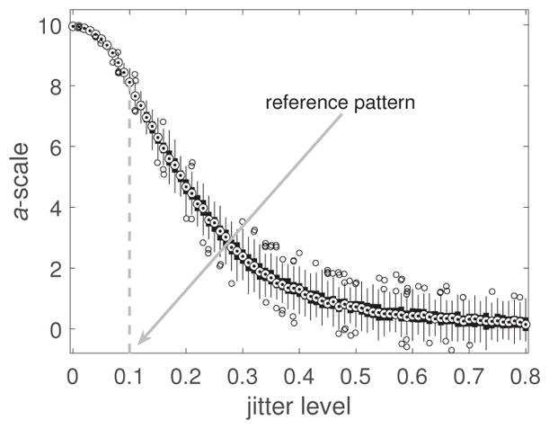
Boxplot of a-scale estimates of perceived regularity for point patterns of 180 points as a function of jitter level. Jitter level is expressed in units of SD of the Gaussian jitter as a fraction of dot spacing.

The above considerations have been taken into account in the pattern-selection process. Since we are interested in discrimination performance and a large amount of data per observer is required, we had to restrict our analysis to a narrow range of the regularity spectrum. We thus decided to use a single reference pattern. The corresponding jitter level was selected as 0.1 as this value lies on the linear section of the curve (Figure 5). Moreover, the slope has its maximum value allowing us to use a small range of jitter values to estimate discrimination performance. This reference pattern is closer to the regular end of the scale, which results in reduced pattern variability. The linearity and the narrow range in jitter allow us to fit a cumulative Gaussian psychometric function to the data. Additionally, judgments between more regular patterns are easier for observers.

In pilot studies, even at this low level of jitter, pattern variability was considerable. We decided to further reduce this variability by pre-selecting patterns. We pregenerated 1,000 patterns for each jitter level (spacing of 5× 10⁻⁴). Since it appears in all trials, for the reference pattern we generated a larger number (10,000). We selected patterns from these sets that differ from the mean of the group by less than 0.1 units on the a-scale. If this selection using the a-scale biases perceived regularity, it should do so similarly for all conditions at a given jitter level, and hence comparisons across conditions should remain valid.

As jitter increases, a larger number of dots will be displaced out of the selected subregion of the pattern, but a larger number of dots will be displaced into the subregion as well. Given the finite size of our patterns, we examined whether this stochastic fluctuation resulted in a significant bias of dot number across jitter levels. We found that there was a slight increase of average dot number as jitter increased. The average numbers of dots and corresponding 95% confidence intervals were 150±4 for the reference pattern and 148±3 and 151±4 for the two extreme jitter values of the test patterns (0.05 and 0.15), respectively. These variations are quite small, thus we do not expect that regularity judgments are confounded with variations in the number of dots, particularly given that the most relevant data for the computation of sensitivity were located much closer to the reference pattern than the two extremes. Additionally, as mentioned above, a common urn of xy-coordinates was employed to depict (appropriately scaled) patterns across conditions. Thus, judgments cannot be biased due to pattern specifics across conditions. Note also that the estimation of peakedness of a condition is based on the range of our measure from a perfect lattice to a Poisson pattern, neither of which was included in the stimulus set. The estimation of peakedness is robust both with respect to the pattern dot number and the size of the second-stage summation filter. This is because the response curves are rescaled to match at the peak that corresponds to the individual dots.

2.1.4 Conditions

There were 7 conditions in the experiment, corresponding to different values of dot size and spacing (Table 1). Dot size values were multiples of d = 3.24 arcmin (2 pixels) and dot spacing values were multiples of D = 32.4 arcmin (20 pixels). Pattern radius was proportional to dot spacing (where R = 3.77 deg) to maintain a constant number of dots. With these limitations we generated a number of conditions and selected ones that spanned the range of peakedness. The last row in Table 1 shows the peakedness value computed as described in the Introduction. In our analysis we varied spatial frequency f over a broad range, setting the bandwidth b of the filter to one octave, consistent with values found in the literature (Blakemore & Campbell, 1969; Stromeyer & Klein, 1974; De Valois, Albrecht & Thorell, 1982; Foster, Gaska, Nagler & Pollen, 1985). One octave is narrow enough to allow the identification of clear peaks in the spectrum of responses across scale for our stimuli. However, our results are robust with respect to the bandwidth setting.

Table 1.

Conditions for experiment 1 (d = 3.24 arcmin, D = 32.4 arcmin, R = 3.77 deg)

Condition	1	2	3	4	5	6	7
Dot size	d	d	d	2d	2d	4d	4d
Dot size (mm)	0.54	0.54	0.54	1.08	1.08	2.16	2.16
Dot spacing	D	23/4D	2D	D	2D	23/4D	2D
Dot spacing (mm)	5.4	9.1	10.8	5.4	10.8	9.1	10.8
Pattern radius	R	23/4R	2R	R	2R	23/4R	2R
Peakedness	0.70	0.44	0.38	1.04	0.56	1.10	0.94

2.1.5 Procedure

Observers were presented with two dot patterns, centered 8.6 deg to the left and right of the display center (Figure 6). One was a reference pattern (jitter = 0.1) and one was a comparison pattern. They selected by keypress the pattern that appeared to be more regular (2AFC). A small black fixation cross was presented before each trial at the center of the screen, and test and reference patterns were randomly positioned to the left or right. To avoid learning of the patterns, images were displayed rotated by 0, 90, 180 or 270 deg, chosen randomly. The duration of presentation was 1500 ms. Observers had unlimited time to register a response after the end of the presentation. Auditory feedback was provided after each trial. The next trial was initiated 500 ms after the response.

Figure 6.

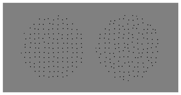
Experiment 1: Sample stimulus display.

The jitter level of the comparison stimulus was controlled by four interleaved staircases (Levitt, 1971). Two were 1-up/2-down (converging on 71%) and two were 2-up/1-down (converging on 29%). The initial step was 16 times the smallest step size (5 × 10⁻⁴). Step size was halved at every reversal of each staircase until it reached the minimum. The starting values of jitter for the staircases were 0.05 for the 2-up-1-down and 0.15 for the 1-up-2-down staircases. During each session, 5 easy trials with extreme values (0.05 and 0.15) were included on randomly chosen trials to remind the observer of the nature of the task and also to stabilize estimates of the lapse rate to avoid biased estimates of the slope of the fitted psychometric curve (Prins, 2012).

Each session consisted of 7 blocks of trials (one per condition), run in random order. Each block consisted of 150 trials (35 trials per staircase plus 5 easy trials each at the low and high ends of the tested jitter range). Observers 1, 2, and 4 completed six sessions, while observer 3 completed four.

2.2 Results

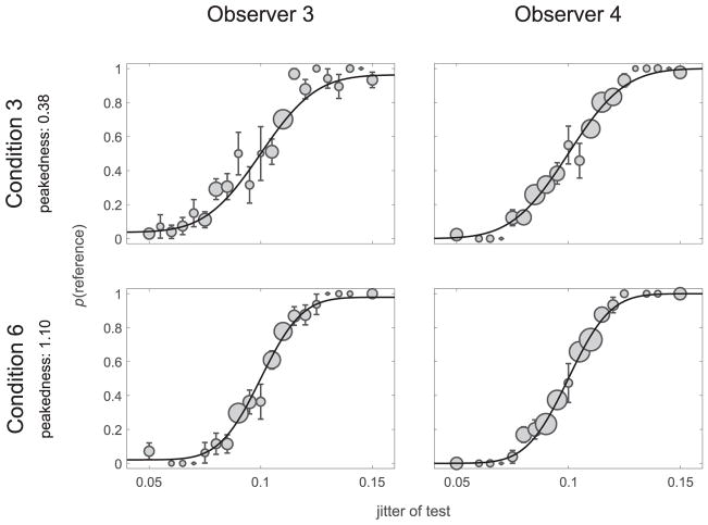
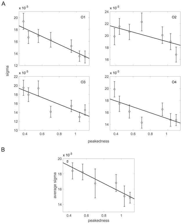
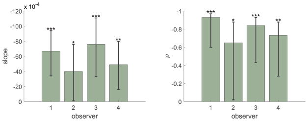
Cumulative Gaussian psychometric functions were fit by maximum likelihood to the probability of selecting the reference stimulus as a function of the comparison stimulus’ jitter value. We included a lapse parameter to minimize estimation bias (Wichmann & Hill, 2001a; Prins, 2012). Each individual and condition was fit separately. Figure 7 shows examples of fitted psychometric curves for conditions 3 and 6, which have the lowest and highest peakedness values, respectively. Data are binned for ease of plotting. The SD (σ) value of the cumulative Gaussian function is an estimate of discrimination performance; lower values of σ correspond to higher sensitivity. Figure 8 shows σ as a function of the peakedness measure for individual observers. Error bars were computed using a parametric bootstrap (1,000 repetitions) (Efron, 1979; Wichmann & Hill, 2001b). The number of simulated trials at each jitter level was identical to the number run by the observer at that level. Figure 9 summarizes linear regression fits to the individual data (slopes and correlation coefficients), confirming the observation that sensitivity increases with peakedness. Confidence intervals of the slopes and correlation coefficients were computed based on 100,000 bootstrapped estimates from the previously bootstrapped values of σ.

Figure 7.

Experiment 1 results. Psychometric curves and data for observers 3 and 4 in conditions 3 (top) and 6 (bottom). The condition with higher peakedness (condition 6) also has steeper slope (i.e., higher sensitivity). Dot area is proportional to the number of trials per datapoint. Error bars: ±1 standard error.

Figure 8.

Experiment 1 results. (A) σ vs. peakedness for the four observers (O1–O4). Error bars: ±1 standard error. (B) Average σ across observers as a function of peakedness. Solid lines: linear regression fits to the data. Error bars: ±1 standard error of the mean across observers.

Figure 9.

Experiment 1 results. Slope and correlation coefficient, ρ, for the four observers. Error bars: 95% confidence intervals. (*: p < 0.05; **: p < 0.01; * * *: p < 0.001)

Considering the data jointly across observers, we performed a linear-mixed effects analysis of the relationship between discriminability and peakedness. We used the lme4 package (Bates, Mächler, Bolker & Walker, 2015) in the R environment (R Core Team, 2015). We treated peakedness as a fixed effect and intercepts and slopes by observer as random effects. We included the maximal random-effects structure as, in general, this approach is more conservative and results in lower Type I error rate than fixed slopes (Barr, Levy, Scheepers & Tily, 2013). The estimated slope is (−58±10)×10⁻⁴. The p-value obtained by a likelihood ratio test of the full model with the peakedness effect included and a null model without the effect is p = 0.002. The Pearson correlation coefficient between peakedness and σ averaged across observers (Figure 8) is ρ = −0.95 (p = 8×10⁻⁴). These results strongly confirm our hypothesis that larger peakedness values result in greater sensitivity to regularity across a set of stimuli.

3 Experiment 2

While the results of Experiment 1 provide support for the hypothesis that regularity is coded via the peakedness of the distribution of responses across scale, we have only examined discrimination performance relative to a single reference point of regularity. To examine whether the dependence of discriminability on peakedness is not specific to this small range of regularity, we conducted Experiment 2 to analyze discrimination performance across the entire range of regularity.

3.1 Methods

In our previous work (Protonotarios et al., 2016), patterns consisted of 180 dots of diameter 3.44 min, which were displayed within a circle of radius 4.58 deg. For these presentation conditions, we showed that humans can distinguish up to 16.5 JNDs of regularity across the entire range. Here, we are interested in whether this JND range increases with increasing peakedness. We describe scaling experiments, ten in total, for different presentation conditions, attempting to achieve reasonable variation in discriminability. All were based on the same 2AFC task as in Experiment 1. Only patterns with the same presentation parameters were compared with each other.

3.1.1 Observers

Ten observers (age: 19–41, four females) participated in the experiment. One was the first author, and the rest were undergraduate or graduate students at the University of London and naïve to the purpose of the experiment. Six completed both stages of the experiment while two reinvited participants of the first stage (Groups A and B) were not available and were replaced. All reinvited participants carried out the second part of the experiment within less than six days of the first. All reported normal or corrected-to-normal vision. Ethical approval for the study was obtained from the UCL Experimental Psychology Departmental Ethics Committee (CPB/2010/003). Participants gave informed consent prior to the experiment. All procedures were carried out in accordance with the Code of Ethics of the World Medical Association (Declaration of Helsinki).

3.1.2 Apparatus

Stimuli for all conditions were presented on a 40 cm diagonal LCD laptop screen (Lenovo ThinkPad W520) under comfortable room illumination. The screen resolution was 1920 × 1080 pixels and the viewing distance was approximately 50 cm. At this distance one pixel (0.18 mm) corresponds to visual angle of 0.021 deg. Each pattern was rendered using solid black dots on a white circular disk (206.0 cd/m²). As in experiment 1, dots were drawn with anti-aliasing. Patterns were displayed in pairs on a grey background (40.4 cd/m²) with their centers at the same height separated horizontally by 19.6 deg (Figure 10). Presentation of stimuli and recording of responses were controlled using the MATLAB Psychtoolbox software (Brainard, 1997).

Figure 10.

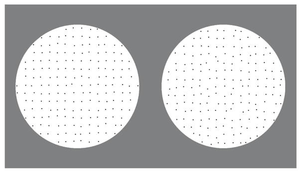
Experiment 2: Sample stimulus display.

3.1.3 Conditions

Conditions were organized into three groups (A, B, and C; Table 2). In Groups A and B (conditions 1 to 7), we varied peakedness by manipulating dot size while keeping dot spacing fixed. In Group A dot size varied, while dot number remained constant (180); in Group B dot number varied while dot size and spacing remained constant, resulting in a fixed peakedness value. The very small variation in peakedness is due to border effects. After analyzing the derived discrimination scales for these 7 conditions, we implemented three additional conditions (Group C, conditions 8–10). We used dot size and number values from conditions 1 to 7, and varied dot spacing to control peakedness. We manipulated the dot spacing for the large dot sizes (0.8 and 1 mm) with high peakedness values and the smallest dot size (0.6 mm), which had low peakedness. Due to limited display size, for the larger dot spacings (conditions 8, 9) the number of dots had to be reduced (to 125). We used the largest dot spacing possible to generate low values of peakedness for the two conditions that previously were associated with high peakedness. The largest dot size (1.2 mm) required even larger dot spacing to achieve a low peakedness value so this size was not used. Conversely, for condition 10, we shrank the pattern for the smallest dot size (0.6 mm) to increase its peakedness and kept the dot number the same as the other two additional conditions (125). For all conditions, the radius of the pattern area was adjusted in accordance with the dot number. The white background was larger than the radius of the pattern by an amount equal to the maximum dot size (1.2 mm or 8.3 min) to ensure that dots were not too close to the border.

Table 2.

Presentation parameters and peakedness values for conditions of Experiment 2. d = 6.90 arcmin, D = 1.09 deg, R = 8.24 deg.

Condition	1	2	3	4	5	6	7	8	9	10
Group	A	A	A, B	A	B	B, C	B	C	C	C
dot size	0.6d	0.8d	d	1.2d	d	d	d	0.8d	d	0.6d
dot size (mm)	0.6	0.8	1.0	1.2	1.0	1.0	1.0	0.8	1.0	0.6
dot spacing	D	D	D	D	D	D	D	1.4D	1.3D	0.6D
dot spacing (mm)	9.5	9.5	9.5	9.5	9.5	9.5	9.5	13.3	12.4	5.7
pattern radius	R	R	R	R	4/6R	5/6R	7/6R	1.17R	1.09R	0.52R
dot number	180	180	180	180	80	125	245	125	125	125
peakedness	0.38	0.45	0.53	0.62	0.52	0.52	0.53	0.32	0.40	0.59

Conditions 1 to 7 were run in random order. The four conditions containing patterns of the default number of dots (180) were interleaved with the three conditions containing patterns with 80, 125, and 245 dots. We excluded orders of conditions that contained sub-sequences with monotonic change in either dot size or dot number to avoid a systematic effect on discrimination performance due to learning or fatigue. Thus, conditions in Group A were not allowed to appear in dot-size order (1, 2, 3, 4, or the reverse, independent of intrusions by the other Group B conditions), and likewise those of Group B were not allowed to occur in dot-number order (5, 6, 3, 7, or the reverse). Conditions 8 to 10 were completed afterward, also in random order.

3.1.4 Stimulus Generation

The stimuli were generated with a method similar to Expt. 1. Patterns were again created using a square lattice and varying amounts of Gaussian positional jitter. The final step of this process was a random selection of a circular window containing the exact specified number of points for the condition. In this experiment patterns of considerable jitter amount were included. Thus, the issue of pattern variability for a given jitter value is particularly important. To reduce variability of perceived regularity within each condition, we again used the a-scale algorithm. In this experiment, we generated a Thurstonian scale based on 2AFC discriminations of regularity among the stimuli in each condition. To do this successfully requires partial overlap of perceived regularity for neighboring stimuli on the scale. We generated a large number of point patterns (1,000) for each of a large number of jitter levels. Each pattern was a circular patch containing exactly 245 points. After computing the corresponding a-scale values, we determined 31 jitter levels that, on average, were uniformly spaced on the a-scale. The uniform spacing of the patterns on the discrimination scale was used to achieve maximum overlap of perceptual regularity estimates on the discrimination scale. For the highest jitter level we generated Poisson point patterns.

Although we are interested in comparing the scales across conditions, we refrained from using a common set of stimuli for all. Extensive exposure to them would induce learning and so judgments would not be independent. Therefore, we pre-selected 10 patterns that had a-scale values close to the mean for each level of jitter. The 10 pre-selected patterns for each jitter level were randomly allocated, one to each of the ten conditions. The 31 patterns for each condition were numbered from ‘1’ to ‘31’ in increasing jitter. We excluded patterns that contained points that would overlap when displayed as dots. To avoid a per-condition bias in this process, we applied the same criteria for all conditions; that is, we checked for overlap assuming the maximum parameter value for dot size and the minimum for dot spacing. For the conditions that required fewer than 245 points, we placed a correspondingly smaller circle on the pattern in random locations until the correct number of points (e.g., 180) fell within the circle, and that sub-pattern was then used in that combination of condition and jitter level.

We cannot predict beforehand the discrimination performance for each presentation condition, so we chose a large number of patterns to ensure sufficient perceptual overlap. Given the high number of patterns and the ten conditions we aimed to examine, to minimize the per-observer number of trials, we excluded uninformative judgments, i.e., those between pairs of large difference in regularity. The resulting design matrix is shown in Figure 11.

Figure 11.

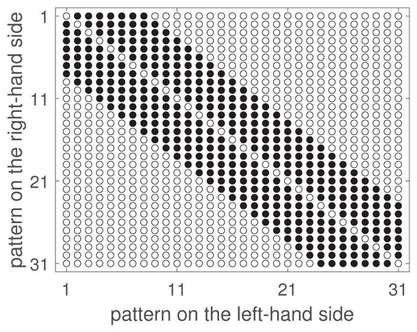
Experimental design matrix for Expt. 2. Patterns are numbered from ‘1’ to ‘31’ in increasing a-jitter amount. Filled disks: pairs included in the experiment (n_pairs = 189). Non-filled disks: excluded pairs.

3.1.5 Task

Written instructions were presented on the display at the beginning of each block. Participants performed a small number of test trials (5–10) before they started the actual experiment. In each trial, two stimuli were displayed until the observer’s response. Observers again selected the more regular pattern by keypress (2AFC). A tone confirmed registration of the response and the next trial started automatically. In contrast to Expt. 1, feedback was not provided. Observers were able to return to previous trials for correction of keystroke errors and were free to control the pace of the experiment. Each of the 189 pairs was presented in random order in two blocks, resulting in 378 comparisons per participant for each condition. For each pair the patterns were randomly allocated to the left or right in the first block, and then in the opposite way in the second block. As in Expt. 1, patterns were randomly rotated by an integer multiple of 90°. Randomization aimed to minimize learning of the patterns and to reduce bias and effects of adaptation (Ouhnana et al., 2013). Across participants, the duration of the two blocks of a given condition ranged from 7 to 21 min.

3.1.6 Thurstonian scaling

We used Thurstonian scaling to estimate a perceptual scale of regularity for the 31 patterns, separately for each condition. Thurstonian scaling provides a convenient way for studying discrimination across a large range of a perceptual attribute. It uses the results of pairwise judgments to place the stimuli on an interval scale. According to this approach, each stimulus S_i has a true value M_i on a numerical scale, and each separate perception of it at trial t, ψ_i,t, is a noisy realization of the true value (M_i + ε_i,t). When two stimuli S_i, S_j are compared, the observer considers the sign of the difference (M_i + ε_i,t) − (M_j + ε_j,t) to report the one that contains a higher amount of the attribute in question. In our case, the perceptual attribute is regularity and the observer reports the more regular stimulus. Assuming that noise is identically distributed and independent, there exists a monotonic preference function P : ℜ → [0, 1] that maps the signed difference between the true values, ΔM = M_i − M_j, to the probability that the one will be preferred to the other. When the noise distributions of the pairs have sufficient overlap, then the preference rates will not all be 0 or 1 and fitting this model to the preference rates may be used to estimate the M_i values. In the case of unit-variance Gaussian noise (Thurstone Case V), the preference function has the form of a cumulative Gaussian distribution (Thurstone, 1927). Other cases have also been suggested, such as Gumbel-distributed noise (the Bradley–Terry Model), resulting in a logistic preference function (Bradley & Terry, 1952; David, 1988). Here, we use the Gaussian model. However, this method of scaling is relatively robust to distributional assumptions (Stern, 1992).

We fit models to data pooled across observers using a maximum-likelihood criterion. Similarly to the psychometric functions of Expt. 1, we rescaled the preference function to incorporate lapses and thus avoid estimation bias due to lapses (Harvey, 1986; Wichmann & Hill, 2001a). The model is parameterized by the unknown true values of perceived regularity of each pattern and the lapse-rate parameter. Thurstonian scales are expressed in steps of the SD of the internal noise. Since they lie on an interval scale, they are invariant under linear transformation. Therefore, we can choose the unit distance to match one just noticeable difference (JND), which we define as the distance between two stimuli that results in a 75% probability of correct ranking (Torgerson, 1958). This definition is equivalent to assuming the standard deviation of ε is 1.048. Only differences in fitted values, not absolute values, are used to predict preference rates. Therefore, without loss of generality we fix the least regular pattern (the Poisson pattern) to have a scale value zero.

3.2 Results

3.2.1 Agreement Rates

We computed two measures of response variability, the intra- and inter - observer agreement rates. The intra-agreement rate expresses the probability that a participant will repeat the same judgment when faced twice with the same pair of stimuli. The inter -agreement rate expresses the probability that two observers’ judgments will agree for the same pair (i.e., the probability that a randomly chosen response from one observer for one trial of a pair agrees with a randomly chosen trial’s response for another observer for the same pair). These rates are shown in Table 3. Agreement rates differ by at most 8% across conditions; they range between 71% and 79%. The intra- and inter - rates do not differ by more than 2%. Thus, there is little variation between participants over and above individual response variability.

Table 3.

Agreement rates.

Condition	1	2	3	4	5	6	7	8	9	10
intra (%)	71	78	73	76	74	76	79	71	72	74
inter (%)	71	76	73	76	74	75	78	71	72	74

3.2.2 Discrimination Scales

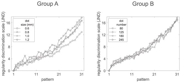
For each condition, we use Thurstonian scaling to learn about the range of discriminability across the entire regularity range, i.e., the difference of the fitted scale values of the two extremes. This difference (in JND units) is our estimate of discrimination performance. In all experiments, pattern ‘1’ has a scale value of zero. Thus, the overall discriminability estimate is simply the highest fitted regularity value. Figure 12 shows the estimated scales for Groups A and B. For Group A, overall discriminability ranges from 12.9 to 17.7 JNDs. The lowest value corresponds to the smallest dot size (0.6 mm), while the highest value corresponds to the largest (1.2 mm). For Group B, overall discriminability differs only slightly between conditions, ranging from 16.7 to 17.8 JNDs.

Figure 12.

Expt. 2: Discrimination scales for the conditions in Groups A (dot spacing: 9.5 mm, dot number: 180) and B (dot spacing: 9.5 mm, dot size: 1.0 mm).

Similarly to previous data shown in Figure 3, for each condition, fitted regularity scale values for patterns ‘1’ to ‘31’ correlate very well with the height of the peak in the distribution of responses at the position associated with the spatial period of the pattern. For conditions 1 and 4 (the conditions with the lowest and highest discriminability over Groups A and B), the Pearson correlation coefficients were 0.98 and 0.97, respectively.

Across conditions (Groups A and B), the correlation between peakedness and discriminability is 0.83 (p = 0.02, Figure 14). However, this value relies mostly on the datapoint of condition 1; discriminability for this condition is considerably lower than in the other conditions. To establish with higher confidence whether a positive correlation exists, we included the additional conditions of Group C.

Figure 14.

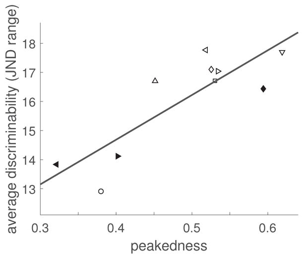
Expt. 2: Linear fit to discrimination performance as a function of peakedness. Non-filled symbols: Conditions of Groups A and B. Filled symbols: Group C-only conditions. Circle: Condition 1. (Symbol correspondence to conditions is consistent with Figures 12 and 13.)

Figure 13 shows the estimated scales for Group C. In comparison to the previous, the performance associated with 0.8 and 1 mm dot sizes is worse (from 16.7 JNDs to 13.8 and 14.1 JNDs respectively). Conversely, performance for the 0.6 mm dot size has improved (from 12.9 to 16.4 JNDs). The signs of these changes are consistent with the peakedness changes for the same dot size. Table 4 shows the average discriminability for all 10 conditions.

Figure 13.

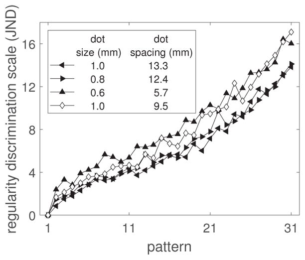
Expt. 2: Discrimination scales for the conditions in Group C. Dot number for all conditions: 125.

Table 4.

Expt. 2: Discrimination performance and peakedness values.

Condition	1	2	3	4	5	6	7	8	9	10
Discriminability (jnd)	12.9	16.7	16.7	17.7	17.8	17.1	17.0	13.8	14.1	16.4
Peakedness	0.38	0.45	0.53	0.62	0.52	0.52	0.53	0.32	0.40	0.59

Neglecting range variation, the discrimination scales look similar for all experimental conditions (Figures 12 and 13) and exhibit an almost linear increase with respect to pattern number as predicted by our a-scale. For this parameter range, discrimination performance is relatively stable. This is interesting given the two-fold change in dot size and three-fold change in dot number.

Across all 10 conditions, the Pearson correlation coefficient between peakedness and discriminability is 0.85 (p = 0.002), i.e., the linear relationship describes a substantial fraction of the variance. Figure 14 shows discrimination performance values against peakedness and the linear fit.

In the first experiment we showed that discriminability and peakedness are highly correlated. However, a single reference value of regularity was used. To generalize our results we conducted Thurstonian scaling extending across the entire range of regularity using perfect regularity and total randomness as anchor points. This allowed us to compare the scales for different conditions. The latter comparison (Figure 14), however, depends on the average discrimination performance across different levels of regularity and does not depend on how that discriminability is distributed across the scale. Next, we examine whether peakedness differences affect discriminability in a uniform way across regularity. Non-uniformity might result from observers using a different strategy or mechanism for judging regularity for patterns that are highly regular (i.e., lattice-like) as compared to those that are nearly random.

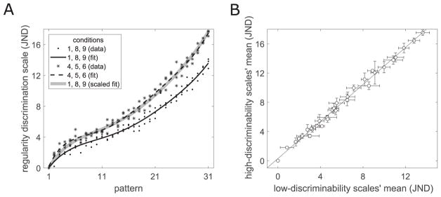
To test for a non-uniform effect of the parameters on discrimination performance, we compared the data from the conditions exhibiting strong discriminability to the data for conditions with poor discriminability. To improve the power of this comparison, we combined the data from three high-discriminability conditions (conditions: 4, 5, 6) and from three low-discriminability conditions (conditions: 1, 8, 9). We ask whether the scale values for one group are proportional to those in the other group. We fit a 6^th-order polynomial to each group of conditions by least squares (Figure 15A). Rescaling the low-discriminability curve results in almost perfect coincidence with the high-discriminability curve. This implies a uniform increase in discrimination sensitivity across the entire regularity range. A scatterplot of the low- vs. high-discriminability scales (one point for each of the 31 jitter levels) confirms this result (Figure 15B).

Figure 15.

Comparison of the disciminability scales for strong- and poor-performance conditions across the entire range of regularity. (A) Combined discrimination scales and polynomial fits for conditions of low (1, 8, 9) and high (4, 5, 6) discriminability. A rescaled polynomial fit of the low-discriminability conditions coincides almost perfectly with the polynomial fit to the high-discriminability conditions. (B) Scatterplot and linear fit of the means of the low- vs. high-discriminability scale values (error bars show standard deviation for the three values for each pattern number).

Note that observers were free to control the pace of their judgments. To confirm that differences in discrimination performance across conditions were not the result of variation in trial duration, we estimated the correlation of trial duration with discriminability across conditions. This correlation is negative, but not significantly different from 0 (Pearson correlation coefficient ρ = −0.26, 95% CI: [−0.77, 0.47]). On average, observers did not spend more time on the conditions yielding strong discrimination performance, and thus, better disciminability cannot be attributed to longer viewing times.

4 Discussion

We have shown that a simple measure of peakedness of the distribution of neural responses across scale correlates with regularity discriminability across different presentation conditions. Our experiments test the peakedness model of regularity coding, and our results are consistent with it.

The analysis, as in Ouhnana et al. (2013), has been based on one dimension considering only vertically oriented Gabors of varying scale since the patterns have an obvious overall orientation and rotational symmetry of 90°. We did not need to consider the responses of neurons tuned to oblique orientations, which may be taken into account by the visual system for patterns of high irregularity.

The suggested measure of peakedness is a straightforward characterization of the distribution of responses across scale. These distributions have at most two peaks, so the relative peak height is a sufficient measure for this class of stimuli. Although convenient and simple, we are not suggesting that this is the actual computation that the visual system utilizes. Its inadequacy becomes obvious by considering more complex stimuli, e.g., textures, which have a greater diversity of response distributions and yet we can nonetheless make judgments of relative regularity for such images. In previous work we compared the discrimination (Thurstone, 1927) and appearance-difference (Maloney & Yang, 2003) scales of regularity for the same class of patterns examined here. We found that if a single mechanism is employed for appearance and discrimination tasks, this would require a source of internal noise that increases for patterns with greater irregularity (Protonotarios, Johnston & Griffin, 2016). This is equivalent to a nonlinear relationship between interval scales based on discrimination vs. appearance judgments. To develop a more general model of the perception of regularity will require consideration of the form of internal noise present in the encoding and read-out mechanisms to model discrimination performance across different levels of regularity.

We have considered a simple class of stimuli based on a perfectly periodic grid and a one-dimensional manipulation of regularity (jitter). This manipulation leaves long-distance correlations intact, retaining phase coherence across the entire pattern. There are many ways to distort perfect symmetry resulting in pattern subregions with varying statistical properties. As such, a successful model of regularity should take into account both local and global features, providing a balance between integration and segmentation. For our uniform patterns, the second-stage filter can encompass the entire pattern, yielding a more stable estimate of regularity. For non-uniform patterns, the degree of pooling over space and orientation will be important. Efficient discrimination may require a mechanism that can adjust the spatial extent of pooling (e.g., that takes into account the inter-element spacing), similar to that proposed by Dakin (1997). This idea is consistent with the good agreement with human performance of our geometric algorithm that relies on a Delaunay triangulation for a diverse set of point patterns as compared to an autocorrelation model (Protonotarios et al., 2014).

Dot size and spacing affect the heights and positions of the two peaks in the response distribution. An increase in the average dot spacing results in a leftward shift and reduced amplitude of the peak of the response distribution that corresponds to the duty cycle of the pattern. Conversely, as dot spacing decreases, that peak rises and shifts rightward toward the peak corresponding to the individual dot size. When dot spacing and dot size are comparable, the two peaks merge, and the simple read-out mechanism based on peak heights becomes ill-defined. This problem can be ameliorated by reducing the bandwidth of the first-stage filters, but we have used biologically realistic values for first-stage bandwidth. Use of considerably larger elements would be required to test whether discriminability is reduced as the peaks in the response distribution overlap. Our model is based on relative peak height and so another prediction of the model that should be tested is whether perceived regularity is contrast-invariant.

Ouhnana et al. (2013) found that the aftereffect of perceived regularity is uni-directional. That is, a test pattern always appears to be less regular after adaptation to a pattern of similar regularity. Based on this, it was suggested that this results from a norm-based adaptation mechanism (Webster, 2011) where irregularity is the norm. In support of this view, their results show that the strength of the aftereffect depends on the regularity level of the adaptor. In particular, as the adaptor regularity decreases, so does the strength of the aftereffect. However, the decrease is linear, and does not appear like it would reach zero for a maximally irregular adapter. They did not test highly irregular adapters and thus did not check whether such adapters change the direction of the aftereffect. We generated 1000 point patterns with the method of Ouhnana et al. (2013) (i.e., with element jitter that was drawn from a rectangular distribution) for the most irregular adapter they considered. The mean a-scale value was 3.62±0.02. Recall that the a-scale ranges from 0 (Poisson, maximally irregular) to 10 (perfect regularity). Thus, more irregular patterns could have been tested, leaving open the question of whether the aftereffect is always uni-directional. In their study, the effect of the adaptor at this level of regularity seemed minimal (near zero). We next ask whether this pattern bears some special significance. It is closer to the irregular end of the a-scale, which is a discrimination-based scale. However, there is a non-linear mapping between the appearance and discrimination scales (Protonotarios et al., 2016), and this pattern lies approximately in the middle of the perceptual appearance scale, i.e., at equal distance between perfect regularity and total randomness. Thus, perhaps the norm is not irregularity, but rather it is at the middle of the scale of perceived regularity.

Contrary to Ouhnana et al. (2013), Yamada et al. (2013), using dot patterns and the same type of positional jittering, found that the regularity aftereffect is bi-directional. That is, adaptation to a regular pattern can make a test pattern appear less regular, and adaptation to an irregular pattern can make a pattern of medium regularity appear more regular. The authors did not provide any explanation for this difference in results apart from pointing out that the two studies used different numbers of elements [16×16 in Yamada et al. (2013) vs. 7×7 in Ouhnana et al. (2013)]. However, it seems clear that a larger number of elements should not affect the distribution of responses since the patterns are uniform and the final filter stage can only pool across more elements for the larger pattern. We next ask whether this discrepancy can be attributed to the use of a more irregular adaptor by Yamada et al. (2013). We generated 1000 patterns with the same method as before and found that the most irregular adaptor used by Yamada et al. (2013) was of the same level of regularity (3.63±0.02 on the a-scale) as the one used by Ouhnana et al. (2013). This is puzzling, since in the first study this pattern causes test stimuli to appear more irregular, while in the second study they appear more regular. We next provide an explanation that is consistent with both studies and consider its testable predictions for future research.

When adaptation occurs for a high-level stimulus attribute, this need not imply that sensitivity was reduced at a high level of the visual stream where that feature is encoded. Sensitivity modulation in response to adaptation may occur at one or several lower levels of processing (Webster, 2011). The site of adaptation can be tested experimentally. For example, Yamada et al. (2013) tested whether adaptation to a pattern rotated by 22.5° led to a regularity aftereffect, and found that it did not. They concluded that regularity is not coded by the relative position of the pattern elements, as in geometric measures of regularity based on point coordinates. However, the absence of adaptation in response to the rotated adaptor suggests that the aftereffects in the two studies rely on changes in earlier orientation-selective stages of vision. Identifying the norm for adaptation based on a high-level attribute is misleading if the site of adaptation is at an earlier stage of processing. Ouhnana et al. (2013) suggested that the regularity aftereffect was a consequence of contrast normalization (Carandini & Heeger, 2011) that aims to equate responses across orientation and scale. Note, however, that a common normalization factor for the whole population of neurons would only scale the responses without altering the shape of the distribution. Further, they assumed that the flattest response distribution corresponds to the most irregular pattern. Thus, they identified irregularity as the norm. This is not true in general: the shape of the response distribution depends on the level of regularity, which controls the duty-cycle peak height, but also on the relative sizes of the element and element spacing. This is crucial for explaining the discrepancy between the two studies; these parameters were different, with much larger element-spacing relative to element size in the study of Yamada et al. (2013).

Figure 16 displays the peaks of the distribution of neural responses for patterns with two different element spacings and three different levels of regularity. Adaptation can be thought of as a homeostatic mechanism that pushes responses in the direction of a standard, unadapted state (Benucci, Saleem & Carandini, 2013). Also plotted in the figure is a putative flat distribution that might be used as the asymptotic distribution or “goal” of adaptation. For large spacing (the left-most region of spatial frequencies), all response-distribution peaks are below the flat distribution. Thus, for such a spacing, adaptation should push peaks upward, and hence lead to a uni-directional effect that makes all patterns appear more regular. For the small element spacing (middle region in the figure), all peaks lie above the flat distribution, and hence adaptation would push peaks downward, resulting in a uni-directional adaptation aftereffect making all patterns appear more irregular. For an intermediate spacing, this same logic would predict a bi-directional effect: Irregular patterns would appear more regular and vice versa, as reported by Yamada et al. (2013). Thus, this view reconciles the contradictory results reported by the two studies and makes testable predictions about the direction and strength of aftereffects.

Figure 16.

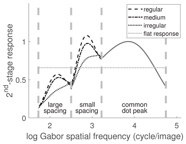
Neural-response peaks associated with the pattern for two element spacings and three levels of regularity. The flat line represents the global average response. If adaptation tries to push responses toward this global average, it predicts opposite effects for patterns with small vs. large element spacings.

Point patterns appear in scientific research in the analysis of evolving systems. They are commonly visually examined for assessment of regularity. Our results suggest that using a larger dot size will yield higher peakedness values and therefore should facilitate regularity comparisons.

5 Conclusion

In this work we examined whether a peakedness model for regularity coding, originally proposed by Ouhnana and colleagues (2013), is consistent with regularity discriminability for dot patterns across varying presentation conditions. We focused on a class of point patterns with a simple type of translational symmetry and varied the degree of regularity by introducing different levels of positional jitter. We used two different methods. The first used a single reference jitter level and examined discriminability near that reference level. The second method extended the analysis to the full spectrum of regularity from perfect regularity to total randomness, and employed Thurstonian scaling. The results of both experiments were consistent with the model: higher peakedness, as quantified using our simple proposed peakedness measure, results in higher discrimination performance. This finding has a practical application: for visual assessment of regularity in dot patterns, the use of larger dots will enhance discrimination.

References

- Allïk J, Tuulmets T. Occupancy model of perceived numerosity. Perception & Psychophysics. 1991;49:303–314. doi: 10.3758/bf03205986. [DOI] [PubMed] [Google Scholar]
- Attneave F. Some informational aspects of visual perception. Psychological Review. 1954;61:183–193. doi: 10.1037/h0054663. [DOI] [PubMed] [Google Scholar]
- Barr DJ, Levy R, Scheepers C, Tily HJ. Random effects structure for confirmatory hypothesis testing: Keep it maximal. Journal of Memory and Language. 2013;68 doi: 10.1016/j.jml.2012.11.001. [DOI] [PMC free article] [PubMed] [Google Scholar]
- Bates D, Mächler M, Bolker B, Walker S. Fitting linear mixed-effects models using lme4. Journal of Statistical Software. 2015;67:1–48. [Google Scholar]
- Benucci A, Saleem AB, Carandini M. Adaptation maintains population homeostasis in primary visual cortex. Nature Neuroscience. 2013;16(6):724–729. doi: 10.1038/nn.3382. [DOI] [PMC free article] [PubMed] [Google Scholar]
- Bertamini M, Zito M, Scott-Samuel NE, Hulleman J. Spatial clustering and its effect on perceived clustering, numerosity, and dispersion. Attention, Perception, & Psychophysics. 2016;78:1460–1471. doi: 10.3758/s13414-016-1100-0. [DOI] [PMC free article] [PubMed] [Google Scholar]
- Blakemore C, Campbell FW. On the existence of neurones in the human visual system selectively sensitive to the orientation and size of retinal images. The Journal of Physiology. 1969;203:237–260. doi: 10.1113/jphysiol.1969.sp008862. [DOI] [PMC free article] [PubMed] [Google Scholar]
- Bonneh Y, Reisfeld D, Yeshurun Y. Quantification of local symmetry: application to texture discrimination. Spatial Vision. 1994;8:515–530. doi: 10.1163/156856894x00152. [DOI] [PubMed] [Google Scholar]
- Bradley RA, Terry ME. Rank analysis of incomplete block designs: I. The method of paired comparisons. Biometrika. 1952;39:324–345. [Google Scholar]
- Brainard DH. The psychophysics toolbox. Spatial Vision. 1997;10:433–436. [PubMed] [Google Scholar]
- Burgess A, Barlow HB. The precision of numerosity discrimination in arrays of random dots. Vision Research. 1983;23:811–820. doi: 10.1016/0042-6989(83)90204-3. [DOI] [PubMed] [Google Scholar]
- Carandini M, Heeger DJ. Normalization as a canonical neural computation. Nature reviews Neuroscience. 2011;13:51–62. doi: 10.1038/nrn3136. [DOI] [PMC free article] [PubMed] [Google Scholar]
- Cliffe MJ, Goodwin AL. Quantification of local geometry and local symmetry in models of disordered materials. Physica Status Solidi (b) 2013;250:949–956. [Google Scholar]
- Cohen M, Baum B, Miodownik M. The importance of structured noise in the generation of self-organizing tissue patterns through contactmediated cell-cell signalling. Journal of the Royal Society Interface. 2011;8:787–798. doi: 10.1098/rsif.2010.0488. [DOI] [PMC free article] [PubMed] [Google Scholar]
- Cohen M, Georgiou M, Stevenson NL, Miodownik M, Baum B. Dynamic filopodia transmit intermittent delta-notch signaling to drive pattern refinement during lateral inhibition. Developmental Cell. 2010;19:78–89. doi: 10.1016/j.devcel.2010.06.006. [DOI] [PubMed] [Google Scholar]
- Cook JE. Spatial regularity among retinal neurons. In: Chalupa LM, Werner JS, editors. The Visual Neurosciences. Cambridge, Mass: MIT Press; 2004. pp. 463–477. [Google Scholar]
- Cousins JB, Ginsburg N. Subjective correlation and the regular-random numerosity illusion. The Journal of General Psychology. 1983;108:3–10. doi: 10.1080/00221309.1983.9711472. [DOI] [PubMed] [Google Scholar]
- Dakin SC. The detection of structure in glass patterns: Psychophysics and computational models. Vision Research. 1997;37:2227–2246. doi: 10.1016/s0042-6989(97)00038-2. [DOI] [PubMed] [Google Scholar]
- David HA. The Method of Paired Comparisons. New York: Oxford University Press; 1988. [Google Scholar]
- De Valois RL, Albrecht DG, Thorell LG. Spatial frequency selectivity of cells in macaque visual cortex. Vision Research. 1982;22:545–559. doi: 10.1016/0042-6989(82)90113-4. [DOI] [PubMed] [Google Scholar]
- Delaunay B. Sur la sphère vide. Izvestia Akademii Nauk SSSR, Otdelenie Matematicheskikh i Estestvennykh Nauk. 1934;7:793–800. [Google Scholar]
- Demeyer M, Machilsen B. The construction of perceptual grouping displays using GERT. Behavior Research Methods. 2012;44:439–446. doi: 10.3758/s13428-011-0167-8. [DOI] [PubMed] [Google Scholar]
- Dunleavy AJ, Wiesner K, Royall CP. Using mutual information to measure order in model glass-formers. 2012 doi: 10.1103/PhysRevE.86.041505. arXiv:1205.0187. [DOI] [PubMed] [Google Scholar]
- Efron B. Bootstrap methods: Another look at the jackknife. The Annals of Statistics. 1979;7:1–26. [Google Scholar]
- Foster KH, Gaska JP, Nagler M, Pollen DA. Spatial and temporal frequency selectivity of neurones in visual cortical areas V1 and V2 of the macaque monkey. The Journal of Physiology. 1985;365:331–363. doi: 10.1113/jphysiol.1985.sp015776. [DOI] [PMC free article] [PubMed] [Google Scholar]
- Ginsburg N. Effect of item arrangement on perceived numerosity: Randomness vs regularity. Perceptual and Motor Skills. 1976;43:663–668. doi: 10.2466/pms.1976.43.2.663. [DOI] [PubMed] [Google Scholar]
- Ginsburg N. The regular-random numerosity illusion: rectangular patterns. The Journal of General Psychology. 1980;103:211–216. doi: 10.1080/00221309.1980.9921000. [DOI] [PubMed] [Google Scholar]
- Ginsburg N, Goldstein SR. Measurement of visual cluster. The American Journal of Psychology. 1987;100:193–203. [PubMed] [Google Scholar]
- Glass L. Moire effect from random dots. Nature. 1969;223:578–580. doi: 10.1038/223578a0. [DOI] [PubMed] [Google Scholar]
- Graham NV. Beyond multiple pattern analyzers modeled as linear filters (as classical V1 simple cells): Useful additions of the last 25 years. Vision Research. 2011;51:1397–1430. doi: 10.1016/j.visres.2011.02.007. [DOI] [PubMed] [Google Scholar]
- Griffin LD. Symmetries of 2-D images: Cases without periodic translations. J Math Imaging Vis. 2009;34:259–269. [Google Scholar]
- Harvey LO. Efficient estimation of sensory thresholds. Behavior Research Methods, Instruments, & Computers. 1986;18:623–632. [Google Scholar]
- Jiao Y, Lau T, Hatzikirou H, Meyer-Hermann M, Corbo JC, Torquato S. Avian photoreceptor patterns represent a disordered hyperuniform solution to a multiscale packing problem. Physical Review. E, Statistical, Nonlinear, and Soft Matter Physics. 2014;89(2):022721. doi: 10.1103/PhysRevE.89.022721. [DOI] [PMC free article] [PubMed] [Google Scholar]
- Koffka K. Principles of Gestalt Psychology. New York: Routledge; 1935. [Google Scholar]
- Levitt H. Transformed up-down methods in psychacoustics. Journal of the Acoustical Society of America. 1971;49:467–477. [PubMed] [Google Scholar]
- Machilsen B, Wagemans J, Demeyer M. Quantifying density cues in grouping displays. Vision Research. 2015;126:207–219. doi: 10.1016/j.visres.2015.06.004. [DOI] [PubMed] [Google Scholar]
- Maloney LT, Yang JN. Maximum likelihood difference scaling. Journal of Vision. 2003;3:573–585. doi: 10.1167/3.8.5. [DOI] [PubMed] [Google Scholar]
- Marinari E, Mehonic A, Curran S, Gale J, Duke T, Baum B. Live-cell delamination counterbalances epithelial growth to limit tissue overcrowding. Nature. 2012;484:542–545. doi: 10.1038/nature10984. [DOI] [PubMed] [Google Scholar]
- Miller W. Symmetry Groups and Their Applications. New York: Academic Press; 1972. [Google Scholar]
- Morgan MJ, Mareschal I, Chubb C, Solomon JA. Perceived pattern regularity computed as a summary statistic: implications for camouflage. Proceedings of the Royal Society B-Biological Sciences. 2012;279:2754–2760. doi: 10.1098/rspb.2011.2645. [DOI] [PMC free article] [PubMed] [Google Scholar]
- O’Keeffe M, Hyde BG. Crystal Structures I. Patterns and Symmetry. 1. Washington, D.C: Mineralogical Society of America; 1996. [Google Scholar]
- Ouhnana M, Bell J, Solomon JA, Kingdom FAA. After-effect of perceived regularity. Journal of Vision. 2013;13(8):18. doi: 10.1167/13.8.18. [DOI] [PubMed] [Google Scholar]
- Prins N. The psychometric function: the lapse rate revisited. Journal of Vision. 2012;12(6):25. doi: 10.1167/12.6.25. [DOI] [PubMed] [Google Scholar]
- Protonotarios ED, Baum B, Johnston A, Hunter GL, Griffin LD. An absolute interval scale of order for point patterns. Journal of the Royal Society: Interface. 2014;11:20140342. doi: 10.1098/rsif.2014.0342. [DOI] [PMC free article] [PubMed] [Google Scholar]
- Protonotarios ED, Johnston A, Griffin LD. Difference magnitude is not measured by discrimination steps for order of point patterns. Journal of Vision. 2016;16(9):2. doi: 10.1167/16.9.2. [DOI] [PubMed] [Google Scholar]
- R Core Team. R: A Language and Environment for Statistical Computing. Vienna, Austria: R Foundation for Statistical Computing; 2015. [Google Scholar]
- Sausset F, Levine D. Characterizing order in amorphous systems. Physical Review Letters. 2011;107:045501. doi: 10.1103/PhysRevLett.107.045501. [DOI] [PubMed] [Google Scholar]
- Steinhardt PJ, Nelson DR, Ronchetti M. Bond-orientational order in liquids and glasses. Physical Review B. 1983;28:784–805. [Google Scholar]
- Stern H. Are all linear paired comparison models empirically equivalent. Mathematical Social Sciences. 1992;23:103–117. [Google Scholar]
- Stevens S. On the theory of scales of measurement. Science. 1946;103:677–680. doi: 10.1126/science.103.2684.677. [DOI] [PubMed] [Google Scholar]
- Stromeyer CF, Klein S. Spatial frequency channels in human vision as asymmetric (edge) mechanisms. Vision Research. 1974;14:1409–1420. doi: 10.1016/0042-6989(74)90016-9. [DOI] [PubMed] [Google Scholar]
- Thurstone LL. A law of comparative judgment. Psychological Review. 1927;34:273–286. [Google Scholar]
- Torgerson WS. Theory and Methods of Scaling. New York: Wiley; 1958. [Google Scholar]
- Truskett TM, Torquato S, Debenedetti PG. Towards a quantification of disorder in materials: Distinguishing equilibrium and glassy sphere packings. Physical Review E. 2000;62:993–1001. doi: 10.1103/physreve.62.993. [DOI] [PubMed] [Google Scholar]
- Vancleef K, Putzeys T, Gheorghiu E, Sassi M, Machilsen B, Wagemans J. Spatial arrangement in texture discrimination and texture segregation. i-Perception. 2013;4(1):36–52. doi: 10.1068/i0515. [DOI] [PMC free article] [PubMed] [Google Scholar]
- Wagemans J, Eycken A, Claessens P, Kubovy M. Interactions between grouping principles in Gabor lattices: Proximity and orientation alignment. Investigative Ophthalmology & Visual Science. 1999;40:S358–S358. [Google Scholar]
- Wagemans J, Wichmann F, Op de Beeck H. Visual perception I: Basic principles. In: Lamberts K, Goldstone R, editors. Handbook of Cognition. London: Sage; 2005. pp. 3–47. [Google Scholar]
- Webster MA. Adaptation and visual coding. Journal of vision. 2011;11(5):3. doi: 10.1167/11.5.3. [DOI] [PMC free article] [PubMed] [Google Scholar]
- Whalen J, Gallistel C, Gelman R. Nonverbal counting in humans: The psychophysics of number representation. Psychological Science. 1999;10:130–137. [Google Scholar]
- Wichmann FA, Hill NJ. The psychometric function: I. Fitting, sampling, and goodness of fit. Perception & Psychophysics. 2001a;63:1293–1313. doi: 10.3758/bf03194544. [DOI] [PubMed] [Google Scholar]
- Wichmann FA, Hill NJ. The psychometric function: II. Bootstrap-based confidence intervals and sampling. Perception & Psychophysics. 2001b;63:1314–1329. doi: 10.3758/bf03194545. [DOI] [PubMed] [Google Scholar]
- Yamada Y, Kawabe T, Miyazaki M. Pattern randomness after-effect. Scientific Reports. 2013;3:2906. doi: 10.1038/srep02906. [DOI] [PMC free article] [PubMed] [Google Scholar]