Stacked Generalization: An Introduction to Super Learning

Abstract

Stacked generalization is an ensemble method that allows researchers to combine several different prediction algorithms into one. Since its introduction in the early 1990s, the method has evolved several times into a host of methods among which is the “Super Learner”. Super Learner uses V -fold cross-validation to build the optimal weighted combination of predictions from a library of candidate algorithms. Optimality is defined by a user-specified objective function, such as minimizing mean squared error or maximizing the area under the receiver operating characteristic curve. Although relatively simple in nature, use of Super Learner by epidemiologists has been hampered by limitations in understanding conceptual and technical details. We work step-by-step through two examples to illustrate concepts and address common concerns.

Predicting health-related outcomes is a topic of major interest in clinical and public health settings. Despite numerous advances in methodology in the past two decades, clinical and population health research scientists continue to rely heavily on parametric (e.g., logistic) regression models for prediction. Often, only a single model is specified to generate predictions.

In the early 1990s, Wolpert developed an approach to combine several “lower-level” predictive algorithms into a “higher-level” model with the goal of increasing predictive accuracy.¹ He termed the approach “stacked generalization”, which later became known as “stacking”. Later, Breiman demonstrated how stacking can be used to improve the predictive accuracy in a regression context, and showed that imposing certain constraints on the higher-level model improved predictive performance.² More recently, van der Laan and colleagues proved that, in large samples, the algorithm will perform at least as well as the best individual predictor included in the ensemble.^3–5 Therefore, choosing a large library of diverse algorithms will enhance performance, while creating the best weighted combination of candidate algorithms will further improve performance. Here, best is defined in terms of a bounded loss function, which allows us to define and quantify how well a given algorithm (e.g., regression, machine learning) performs at predicting or explaining the data. Over-fitting is avoided with V -fold cross-validation. In this context, the term “Super Learner” was coined.

Super Learner has tremendous potential for improving the quality of predictions in applied health sciences, and minimizing the extent to which empirical findings rely on parametric modeling assumptions. While the number of simulation studies and applications of Super Learner are growing,^6–14 wider use may be hampered by comparatively few pedagogic examples. Here, we add to prior work by providing step-by-step implementation in the context of two simple settings. We emphasize our goal here is not to showcase the potential gain in predictive power from Super Learner over alternative methods;^6–14 instead, we demonstrate implementation with an aim to confer some intuition on how and why the Super Learner works. Our examples are motivated by common challenges to estimate a dose-response curve, and to build a classifier for a binary outcome. We also link Super Learner to prior work on stacking, provide guidelines on fitting Super Learner to empirical data, and discuss common concerns. Full R code¹⁵ is publicly available at GitHub.

Example 1: Dose-Response Curve

For 1,000 observations, we generate a continuous exposure X by drawing from a uniform distribution with a minimum of zero and a maximum of eight and then generate a continuous outcome Y as

$$Y=5+4\times \sqrt{9X}\times \mathbb{I}(X<2)+\mathbb{I}(X<2)\times ({\left|X-6\right|}^2)+\epsilon ,$$ (1)

where $\mathbb{I}$() denotes the indicator function evaluating to 1 if the argument is true (zero otherwise), and ε was drawn from a doubly-exponential distribution with mean zero and scale parameter one. The true dose-response curve is depicted by the black line in Figure 1. We now manually demonstrate how Super Learner can be used to flexibly model this relation without making parametric assumptions.

Figure 1.

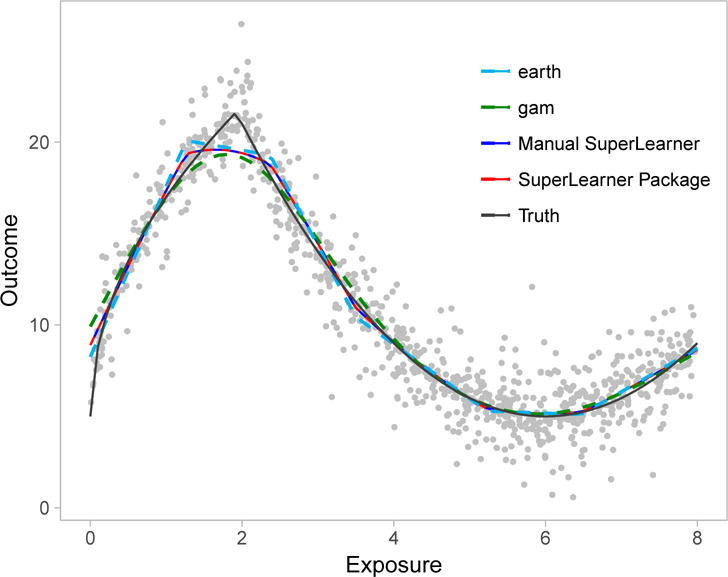
Dose-response curves for the relation between our simulated continuous exposure and continuous outcome in Example 1. The black line represents the true curve, while the red and blue lines represent curves estimated with the programmed Super Learner package in R, and the manually coded Super Learner. Light blue and green curves show the fits from the level-zero algorithms, earth and gam respectively. Gray dots represent observed data-points.

To simplify our illustration, we consider only two “level-zero” algorithms as candidates to the Super Learner library: generalized additive models with 5-knot natural cubic splines ( gam)¹⁶ and multivariate adaptive regression splines implemented via the earth package.²² In practice, a large and diverse library of candidate estimators is recommended. Our specific interest is in quantifying the mean of Y as a (flexible) function of X. To measure the performance of candidate algorithms and to construct the weighted combination of algorithms, we select the L-2 squared error loss function (Y − Ŷ)² where Ŷ denotes our predictions. Minimizing the expectation of the L-2 loss function is equivalent to minimizing mean squared error, which is the same objective function used in ordinary least squares regression.^{17(section 2.4)} To estimate this expected loss, called the “risk”, we use V -fold cross-validation with V = 5 folds. Cross-validation is a sample splitting technique to assess estimator performance using data drawn from the same distribution. As detailed below, each candidate estimator is fit on a portion of the data and used to predict the outcomes for observations that were not used in the training process. As a result, cross-validation helps us avoid poor out-of-sample predictions and gives us a more honest measure of performance. Without this crucial step, we risk generating a predictive algorithm that performs flawlessly for the data at hand, but poorly for another sample. To implement Super Learner, we:

Step 1

Split the observed “level-zero” data into 5 mutually exclusive and exhaustive groups of n/V = 1000/5 = 200 observations. These groups are called “folds”.

Step 2

For each fold v = {1,…,5},

1. Define the observations in fold v as the validation set, and all remaining observations (80% of the data) as the training set.

2. Fit each algorithm on the training set.

3. For each algorithm, use its estimated fit to predict the outcome for each observation in the validation set. Recall the observations in the validation set are not used train each candidate algorithm.

4. For each algorithm, estimate the risk. For the L-2 loss, we average the squared difference between the outcome Y and its prediction Ŷ for all observations in the validation set v. In other words, we calculate the mean squared error (MSE) between the observed outcomes in the validation set and the predicted outcomes based on the algorithms fit on the training set.

Step 3

Average the estimated risks across the folds to obtain one measure of performance for each algorithm. In our simple example, the cross-validated estimates of the squared prediction error are 2.58 for gam and 2.48 for earth.

At this point, we could simply select the algorithm with smallest cross-validated risk estimate (here, earth). This approach is sometimes called the Discrete Super Learner.⁶ Instead, we combine the cross-validated predictions, which are referred to as the “level-one” data, to improve performance and build the “level-one” learner.

Step 4

Let Ŷ_gam-cv and Ŷ_earth-cv denote the cross-validated predicted outcomes from gam and earth, respectively. Recall the observed outcome is denoted Y. To calculate the contribution of each candidate algorithm to the final Super Learner prediction, we use non-negative least squares to regress the actual outcome against the predictions, while suppressing the intercept and constraining the coefficients to be non-negative and sum to 1:

$$\mathbb{E}\left(Y|{\widehat{Y}}_{\text{gam-cv}},{\widehat{Y}}_{\text{earth-cv}}\right)={\alpha }_1{\widehat{Y}}_{\text{gam-cv}}+{\alpha }_2{\widehat{Y}}_{\text{earth-cv}},$$ (2)

such that α₁ ≥ 0; α₂ ≥ 0, and ${\displaystyle {\sum }_{k=1}^2{\alpha }_k=1}$. Combining the Ŷ_gam-cv and Ŷ_earth-cv under these constraints (non-negative estimates that sum to 1) is referred to as a “convex combination,” and is motivated by both theoretical results and improved stability in practice.^2,5 Non-negative least squares corresponds to minimizing the mean squared error, which is our chosen loss function (and thus, fulfills our objective). We then normalize the coefficients from this regression to sum to 1. In our simple example, the normalized coefficient values are ${\widehat{\alpha }}_1=0.387$ for gam and ${\widehat{\alpha }}_2=0.613$ for earth. Therefore, both generalized additive models and regression splines each contribute approximately 40% and 60% of the weight in the optimal predictor.

Step 5

The final step is to use the above weights to generate the Super Learner, which can then be applied to new data (X) to predict the continuous outcome. To do so, re-fit gam and earth on the entire sample and denote the predicted outcomes as Ŷ_gam and Ŷ_earth, respectively. Then combine these predictions with the estimated weights from Step 4:

$${\widehat{Y}}_{\text{SL}}=0.387{\widehat{Y}}_{\text{gam}}+0.613{\widehat{Y}}_{\text{earth}}$$ (3)

where Ŷ_SL denotes our final Super Learner predicted outcome. The resulting predictions are shown in blue in Figure 1. For comparison, the predictions from the R package SuperLearner-v2.0-23-9000 are shown in red,¹⁸ while the predictions from gam and earth are shown in light blue and green, respectively.

Example 2: Binary Classification

Our second example is predicting the occurrence of a binary outcome with goal of maximizing the area under the receiver operating characteristic (ROC) curve, which shows the balance between sensitivity and specificity for varying discrimination thresholds. For 10,000 observations, we generate five covariates X = {X₁,…, X₅} by drawing from a multivariate normal distribution and then generate the outcome Y by drawing from a Bernoulli distribution with probability

$$\mathrm{\mathbb{P}}\left(Y=1|\mathbf{X}\right)=1-\text{expit}\left\{{\beta }_0+{\beta }_1{X}_1+{\beta }_2{X}_2+{\beta }_3{X}_3+{\beta }_4{X}_4+{\beta }_5{X}_5+{\mathit{\beta }}_1\left(X_1:X_5\right)+{\mathit{\beta }}_2{\left(X_1:X_5\right)}_2\right\},$$

where expit(•) = (1 + exp[−•])⁻¹; and (X₁: X₅)₁ and (X₁: X₅)₂ denote all first and second order interactions between X₁,…, X₅, respectively; and β₁ and β₂ denote a set of parameters, one for each interaction. In total, there were 25 terms plus the intercept in this model. The intercept was set to β₀ = 2, while all other parameters were drawn from a uniform distribution bounded by 0 and 1.

Our library of candidate algorithms consists of Bayesian GLMs ( bayesglm), implemented via the arm package (v 1.9-3),²⁰ and multivariate polynomial adaptive regression splines ( polymars) via the polspline package.²¹ Our objective is to generate an algorithm that correctly classifies individuals given covariates. Correct classification is a function of both sensitivity and specificity. Thus, to measure the performance of these level-zero algorithms and build the meta-learner, we use the rank loss function. Instead of minimizing mean squared error, the rank loss function aims to maximize the area under the ROC curve (a function of both sensitivity and specificity), thus optimizing the algorithms ability to correctly classify observations.²³ We again use 5-fold cross-validation to obtain an honest measure of performance and avoid over-fitting.

Steps 1–3

Implementation of Steps 1-3 are analogous to the previous example. In place of gam and earth, we use bayesglm, and polymars. In place of the L-2 loss function, we use the rank loss. Specifically, for each validation set and each algorithm, we estimate the sensitivity, specificity, and then compute the area under the ROC curve (AUC). The expected loss (i.e., “risk”) can then be computed as 1-AUC. Averaging the estimated risks across the folds yields one measure of performance for each algorithm. In our simple example, the cross-validated risk estimates are 0.122 for bayesglm and 0.114 for polymars.

As before, we could simply select the model with lowest cross-validated risk estimate (here, polymars). Instead in Steps 4-5, we combine the resulting cross-validated predictions to generate the level-one learner.

Step 4

Let Ŷ_bglm-cv and Ŷ_pm-cv denote the cross-validated predictions frombayesglm and polymars, respectively. To calculate the contribution of each candidate algorithm to the final Super Learner prediction, use the rank loss function to define “optimal” as the convex combination that maximizes the AUC. Then estimate the α parameters in the following constrained regression

$$\mathrm{\mathbb{P}}(Y=1|{\widehat{Y}}_{\text{bglm-cv}},{\widehat{Y}}_{\text{pm-cv}})={\alpha }_1{\widehat{Y}}_{\text{bglm-cv}}+{\alpha }_2{\widehat{Y}}_{\text{pm-cv}},\text{where}{\alpha }_1\ge 0;{\alpha }_2\ge 0;\text{and}{\displaystyle \sum _{k=1}^2{\alpha }_k=1}$$ (4)

such that (1 − AUC) is minimized when comparing Super Learner predicted probabilities to the observed outcomes. These parameters can be estimated with a tailored optimization function, such as optim in R or proc nlmixed in SAS. In our simple example, the coefficient values are ${\widehat{\alpha }}_1=0.223$ for bayesglm and ${\widehat{\alpha }}_2=0.776$ for polymars.

Step 5

As before, the final step is to use the above coefficients to generate the Super Learner. To do so, refit bayesglm and polymars on the entire sample and denote the predicted outcomes as Ŷ_bglm and Ŷ_pm Then combine these predictions with the estimated weights:

$$\mathrm{\mathbb{P}}\left(Y=1|{\widehat{Y}}_{\text{bglm}},{\widehat{Y}}_{\text{pm}}\right)=0.223{\widehat{Y}}_{\text{bglm}}+0.776{\widehat{Y}}_{\text{pm}}$$ (5)

These predictions can then be used to compute the ROC curve displayed in blue in Figure 2. For comparison the predictions from the R package SuperLearner are shown in red.

Figure 2.

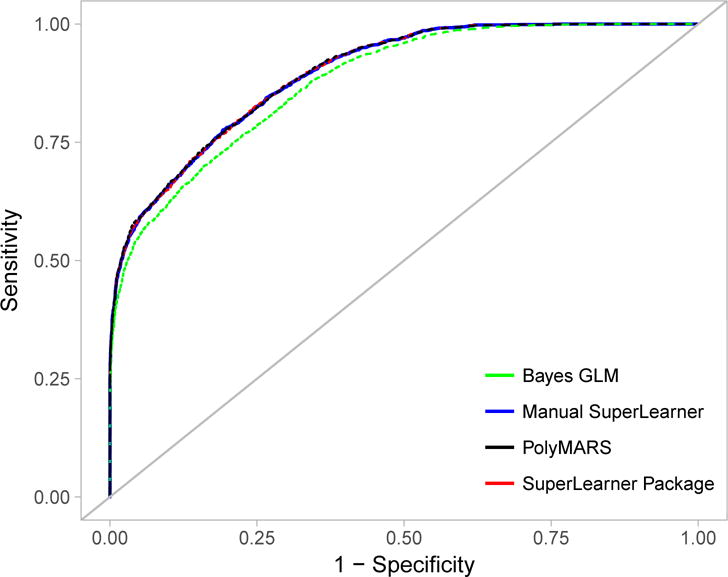
Receiver operating characteristic curves displaying the ability of 5 simulated exposures to predict the simulated outcome in Example 2. Blue line represents the curve obtained from the Super Learner package. Red dotted line represents curve obtained from manually coded Super Learner. The green line represents the curve from level-zero Bayes GLM algorithm, and the black line represents the curve from PolyMARS.

Discussion

Stacked generalizations, notably Super Learner, are fast becoming an important part of the epidemiologic toolkit. There are several challenges in understanding precisely what stacking is, and how it is implemented. These challenges include the use of complex machine learning algorithms as candidate algorithms, and the actual process by which the resulting predictions are combined into the meta-learner. Here, we sought to clarify the latter aspect, namely, implementation of the Super Learner algorithm.

Several considerations (including strengths and limitations) merit attention. First, any number of loss functions could be chosen determine the optimal combination of algorithm-specific predictions. The choice should be based on the objective of the analysis. The target parameter depends on the loss function choice, but various loss functions can identify the same target parameter as minimizer of its risk. Our examples demonstrated the use of the L-2 loss to minimize prediction error when estimating a dose-response curve, and the rank loss to maximize AUC when developing a binary classifier. Other loss functions could be entertained. For example, Zheng et al. recently aimed to simultaneously maximize sensitivity and minimize rate of false positive predictions with application to identify high-risk individuals for pre-exposure prophylaxis.¹⁰

Second, a wide array of candidate algorithms can be included in the Super Learner library. We recommend including standard parametric modeling approaches (e.g., generalized linear models, simple mean, simple median) and more complex data-adaptive methods (e.g., penalized regression, and tree- or kernel-based methods). Often, the performance of data-adaptive methods depends on how tuning parameters are specified. Indeed, tuning a machine learning algorithm is a critical step in optimizing performance, and is straightforward with Super Learner. One need only include the same algorithm in the Super Learner library multiple times, with different tuning parameter values for each candidate entry (e.g., extreme gradient boosting with varying shrinkage rates). We refer the readers to Polley et al.¹⁸ and Kennedy¹⁹ for practical demonstrations of how to deal with tuning parameters.

Third, a critically important part of Super Learning is the use of V -fold cross-validation. However, the optimal choice of V is not always clear. At one end of the extreme, leave-one-out cross validation chooses V = N, but is subject to potentially high variance and low bias. On the other end, 2-fold cross validation is subject to potentially low variance and high bias. A general rule of thumb is to use V = 10.²⁴ Though common, this number will not optimize performance in all settings.²⁵ In general, we recommend increasing the number of folds (V) as sample size n decreases. We also note that other cross-validation schemes (beyond V -fold) are available, even in settings with dependent data.

While Super Learner with a rich set of candidates represents a versatile tool, important limitations should be noted. First, no algorithm (Super Learner or any other machine learning method) should be used to replace careful thinking of the underlying causal structure. Super Learner cannot distinguish between confounders, instrumental variables, mediators, colliders, and the exposure. Instead, the goal of Super Learner is to do the best (as specified through the loss function) possible job predicting the outcome (or exposure) given the inputted variables. Super Learner can, however, minimize assumptions regarding the nature of the relation between the covariates, the exposure, and the outcome. These assumptions are often present in the form of selected link functions, the absence of interactions, and the shape of particular dose-response relations (e.g., linear, polynomial). Nonetheless, if such functional form information is available, this knowledge can readily be included in Super Learner. For example, physicians might prescribe treatments according to a specific algorithm, and this knowledge can be included as a candidate algorithm (e.g. a parametric regression) in Super Learner’s library.

Secondly, Super Learner is a“black box” algorithm; so the exact contribution of each covariate to prediction is unclear. These contributions can be revealed by estimating variable importance measures, which quantify the marginal association between each predictor and the outcome after adjusting for the others. Nevertheless, a large predictor contribution may be the result of direct causation, unmeasured confounding, collider stratification, reverse causation, or some other mechanism.

The goal of prediction is distinct from causal effect estimation, but prediction is often an intermediate step in estimating causal effects.³⁶ Indeed, some researchers have advocated for the use of data-adaptive methods, including Super Learner, for effect estimation via singly-robust methods, depending on estimation of either the conditional mean outcome or the propensity score.^26–32 While flexible algorithms can reduce the risk of bias due to regression model misspecification, a serious concern is that the use of data-adaptive algorithms in this context can result in invalid statistical inference (i.e. misleading confidence intervals). Specifically, there is no theory to support the resulting estimator is asymptotically linear (i.e., consistent and asymptotically normal), which is required to obtain, for example, centered confidence intervals with nominal coverage properties.^33,36 This concern can be alleviated through the use of doubly robust estimators^{34–36,38,39} or higher-order influence function based estimators.^40,41 In contrast, statistical inference is usually not included in prediction algorithms¹⁷ (as in our examples). One could, however, evaluate the performance of Super Learner through an additional layer of cross-validation.⁶

Overall, Super Learner is an important tool that researchers can use to improve predictive accuracy, avoid overfitting, and minimize parametric assumptions. We have provided a simple explanation of Super Learner to facilitate a more widespread use in epidemiology. More advanced treatments with realistic data examples are available^5,7–14,36 and should be consulted for additional depth.

References

- 1.Wolpert D. Stacked generalization. Neural Networks. 1992;5:241–59. [Google Scholar]
- 2.Breiman L. Stacked regressions. Machine Learning. 1996;24:49–64. [Google Scholar]
- 3.van der Laan M, Dudoit S. Technical Report 30. Division of Biostatistics, University of California; Berkeley: 2003. Unified Cross-Validation Methodology For Selection Among Estimators and a General Cross-Validated Adaptive Epsilon-Net Estimator: Finite Sample Oracle Inequalities and Example. [Google Scholar]
- 4.van der Laan M, Dudoit S, van der Vaart AW. The cross-validated adaptive epsilon-net estimator. Statistics & Decision. 2006;24:373. [Google Scholar]
- 5.van der Laan MJ, Polley EC, Hubbard AE. Super learner. Statistical Applications in Genetics and Molecular Biology. 2007;6 doi: 10.2202/1544-6115.1309. Article 25. [DOI] [PubMed] [Google Scholar]
- 6.Polley EC, Rose S, van der Laan MJ. Super Learning. In: van der Laan MJ, Rose S, editors. Targeted Learning: Causal Inference for Observational and Experimental Data. New York Dordrecht Heidelberg London: Springer; 2011. pp. 43–66. [Google Scholar]
- 7.Rose S. Mortality risk score prediction in an elderly population using machine learning. Am J Epidemiol. 2013;177:443–452. doi: 10.1093/aje/kws241. [DOI] [PubMed] [Google Scholar]
- 8.Pirracchio R, Petersen ML, Carone M, Resche Rigon M, Chevret S, van der Laan M. Mortality prediction in intensive care units with the Super ICU Learner Algorithm (SICULA): a population-based study. Lancet Resp Med. 2015;3:42–52. doi: 10.1016/S2213-2600(14)70239-5. [DOI] [PMC free article] [PubMed] [Google Scholar]
- 9.Petersen M, LeDell E, Schwab J, Sarovar MS, et al. Super Learner Analysis of Electronic Adherence Data Improves Viral Prediction and May Provide Strategies for Selective HIV RNA Monitoring. J Acquir Immune Defic Syndr. 2015;69:109–118. doi: 10.1097/QAI.0000000000000548. [DOI] [PMC free article] [PubMed] [Google Scholar]
- 10.Zheng W, Balzer L, van der Laan M, Petersen M, the SEARCH Collaboration Constrained binary classification using ensemble learning: an application to cost-efficient targeted PrEP strategies. Statistics in Medicine. 2017 doi: 10.1002/sim.7296. Early View. [DOI] [PMC free article] [PubMed] [Google Scholar]
- 11.Díaz I, Hubbard A, Decker, Cohen M. Variable Importance and Prediction Methods for Longitudinal Problems with Missing Variables. PloS ONE. 2015;10:e0120031. doi: 10.1371/journal.pone.0120031. [DOI] [PMC free article] [PubMed] [Google Scholar]
- 12.Kreif N, Tran L, Grieve R, De Stavola B, Tasker RC, Petersen M. Estimating the Comparative Effectiveness of Feeding Interventions in the Pediatric Intensive Care Unit: A Demonstration of Longitudinal Targeted Maximum Likelihood Estimation. Am J Epidemiol. 2017;186:1370–1379. doi: 10.1093/aje/kwx213. [DOI] [PMC free article] [PubMed] [Google Scholar]
- 13.Luque-Fernandez MA, Belot A, Valeri L, Ceruli G, Maringe C, Rachet B. Data-Adaptive Estimation for Double-Robust Methods in Population-Based Cancer Epidemiology: Risk differences for lung cancer mortality by emergency presentation. Am J Epidemiol. 2017 doi: 10.1093/aje/kwx317. EarlyView. [DOI] [PMC free article] [PubMed] [Google Scholar]
- 14.Baćak A, Kennedy EH. Principled Machine Learning Using the Super Learner: An Application to Predicting Prison Violence. Sociological Methods & Research. 2018 OnlineFirst. [Google Scholar]
- 15.Core Team R. R: A Language and Environment for Statistical Computing. Vienna, Austria: R Foundation for Statistical Computing; 2017. [Google Scholar]
- 16.Hastie T, Tibshirani R. Generalized Additive Models. London; New York: Chapman & Hall; 1990. [Google Scholar]
- 17.Hastie T, Tibshirani R, Friedman JH. The Elements of Statistical Learning: Data Mining, Inference, and Prediction. New York, NY: Springer; 2009. [Google Scholar]
- 18.Polley E, LeDell E, Kennedy C, van der Laan M. Super Learner: Super Learner Prediction. 2016 URL https://CRAN.R-project.org/package=SuperLearner. R package version 2.0-22.
- 19.Kennedy C. SuperLearner Introduction. 2017 URL https://github.com/ck37/superlearner-guide/blob/master/SuperLearner-Intro.Rmd.
- 20.Gelman Andrew, Su Yu-Sung. arm: Data Analysis Using Regression and Multilevel/Hierarchical Models. 2016 URL https://CRAN.R-project.org/package=arm. R package version 1.9-3.
- 21.Kooperberg Charles. polspline: Polynomial Spline Routines. 2015 URL https://CRAN.R-project.org/package=polspline. R package version 1.1-12.
- 22.Milborrow Stephen. Derived from mda:mars by Trevor Hastie and Rob Tibshirani. Uses Alan Miller’s Fortran utilities with Thomas Lumley’s leaps wrapper. earth: Multivariate Adaptive Regression Splines. 2017 URL https://CRAN.R-project.org/package=earth. R package version 4.5-0.
- 23.Ledell Erin. PhD Dissertation. UC Berkeley: 2015. Scalable Ensemble Learning and Computationally Efficient Variance Estimation. [Google Scholar]
- 24.Kohavi R. A study of Cross-Validation and Bootstrap for Accuracy Estimation and Model Selection. Proceedings of the 14th International Joint Conference on Artificial Intelligence. 1995;2 [Google Scholar]
- 25.Zhang Y, Yang Y. Cross-validation for selecting a model selection procedure. Journal of Econometrics. 2015;187 [Google Scholar]
- 26.Moodie EEM, Stephens DA. Treatment prediction, balance, and propensity score adjustment. Epidemiology. 2017;28 doi: 10.1097/EDE.0000000000000657. [DOI] [PubMed] [Google Scholar]
- 27.Pirracchio R, Carone M. The balance super learner: A robust adaptation of the super learner to improve estimation of the average treatment effect in the treated based on propensity score matching. Stat Methods Med Res. 2016 doi: 10.1177/0962280216682055. 962280216682055. [DOI] [PubMed] [Google Scholar]
- 28.McCaffrey DF, Griffin BA, Almirall D, Slaughter ME, Ramchand R, Burgette LF. A tutorial on propensity score estimation for multiple treatments using generalized boosted models. Stat Med. 2013;32:3388–3414. doi: 10.1002/sim.5753. [DOI] [PMC free article] [PubMed] [Google Scholar]
- 29.Westreich D, Lessler J, Funk MJ. Propensity score estimation: neural networks, support vector machines, decision trees (cart), and meta-classifiers as alternatives to logistic regression. J Clin Epidemiol. 2010;63:826–833. doi: 10.1016/j.jclinepi.2009.11.020. [DOI] [PMC free article] [PubMed] [Google Scholar]
- 30.Lee BK, Lessler J, Stuart EA. Improving propensity score weighting using machine learning. Stat Med. 2010;29:337–346. doi: 10.1002/sim.3782. [DOI] [PMC free article] [PubMed] [Google Scholar]
- 31.Snowden JM, Rose S, Mortimer KM. Implementation of g-computation on a simulated data set: Demonstration of a causal inference technique. Am J Epidemiol. 2011;173:731–738. doi: 10.1093/aje/kwq472. [DOI] [PMC free article] [PubMed] [Google Scholar]
- 32.Westreich D, Edwards JK, Cole SR, Platt RW, Mumford SL, Schisterman EF. Imputation approaches for potential outcomes in causal inference. International Journal of Epidemiology. 2015 doi: 10.1093/ije/dyv135. Published ahead of print July 25, 2015. [DOI] [PMC free article] [PubMed] [Google Scholar]
- 33.van der Vaart A. Higher Order Tangent Spaces and Influence Functions. Statistical Science. 2014;29:679–686. [Google Scholar]
- 34.Robins JM, Rotnitzky A, Zhao LP. Estimation of regression coefficients when some regres-sors are not always observed. Journal of the American Statistical Association. 1994;89:846–866. [Google Scholar]
- 35.van der Laan MJ, Robins JM. Unified Methods for Censored Longitudinal Data and Causality. New York Berlin Heidelberg: Springer-Verlag; 2003. [Google Scholar]
- 36.van der Laan MJ, Rose S. Targeted learning: causal inference for observational and experimental data. New York, NY: Springer; 2011. [Google Scholar]
- 37.Robins JM. Data, design, and background knowledge in etiologic inference. Epidemiol. 2001;12:313–20. doi: 10.1097/00001648-200105000-00011. [DOI] [PubMed] [Google Scholar]
- 38.Naimi AI, Kennedy EH. Nonparametric double robustness. arXiv:1711.07137v1 [stat.ME] [Google Scholar]
- 39.Kennedy EH, Balakrishnan S. Discussion of “Data-driven confounder selection via Markov and Bayesian networks” by Jenny Häggström. Biometrics. 2017 doi: 10.1111/biom.12787. In Press. [DOI] [PubMed] [Google Scholar]
- 40.Robins J, Li L, Tchetgen Tchetgen E, van der Vaart A. Higher order influence functions and minimax estimation of nonlinear functionals. In: Nolan D, Speed T, editors. Probability and Statistics: Essays in Honor of David A Freedman. Beachwood, Ohio, USA: Institute of Mathematical Statistics; 2008. pp. 335–421. Volume 2 of Collections. URL . [DOI] [Google Scholar]
- 41.Diaz I, Carone M, van der Laan MJ. Second-order inference for the mean of a variable missing at random. 2016;12:333. doi: 10.1515/ijb-2015-0031. URL //www.degruyter.com/view/j/ijb.2016.12.issue-1/ijb-2015-0031/ijb-2015-0031.xml. [DOI] [PubMed] [Google Scholar]