

Abstract
The neuroimaging community has seen a renewed interest in algorithms that provide a location-independent summary of subject-specific abnormalities (SSA) to assess individual lesion load. More recently, these methods have been extended to assess whether multiple individuals within the same cohort exhibit extrema in the same spatial location (e.g., voxel or region of interest). However, the statistical validity of this approach has not been rigorously established. The current study evaluated the potential for a spatial bias in the distribution of SSA using several common z-transformation algorithms (leave-one-out [LOO]; independent sample [IDS]; Enhanced Z-Score Microstructural Assessment of Pathology [EZ-MAP]; distribution-corrected z-scores [DisCo-Z]) using both simulated data and DTI data from 50 healthy controls. Results indicated that methods which z-transformed data based on statistical moments from a reference group (LOO, DisCo-Z) led to bias in the spatial location of extrema for the comparison group. In contrast, methods that z-transformed data using an independent third group (EZ-MAP, IDS) resulted in no spatial bias. Importantly, none of the methods exhibited bias when results were summed across all individual elements. The spatial bias is primarily driven by sampling error, in which differences in the mean and standard deviation of the untransformed data have a higher probability of producing extrema in the same spatial location for the comparison but not reference group. In conclusion, evaluating SSA overlap within cohorts should be either be avoided in deference to established group-wise comparisons or performed only when data is available from an independent third group.
Keywords: simulations, single-subject, fractional anisotropy, neuroimaging, overlap
Introduction
There has been an increasing focus (Bouix et al. 2013; Kim et al. 2013; Mayer et al. 2014; Watts et al. 2014) on methods that are capable of identifying individual differences in neuroimaging data (hereafter referred to as subject-specific abnormalities [SSA]). One family of methods uses statistical moments derived from a reference group (RF; typically healthy controls) to z-transform individual subject data in a comparison group (CP; typically patients) and define extrema based on a given statistical threshold. However, the z-transform results in different distributional variances for the transformed data, and as a result over-estimates extrema in CP and under-estimates extrema in RF dependent on sample size (Mayer et al. 2014; Mayer et al. 2017; Watts et al. 2014). This subsequently results in group-wise bias (CP > RF) when comparing the total number of extrema, which is typically amplified by the numerous (i.e., voxelwise) statistical tests that occur in neuroimaging studies.
More recently, a growing number of investigators have examined the spatial overlap of extrema across subjects within individual voxels or regions of interest (ROI) following various z-transform methods (Bouix et al. 2013; Hayes et al. 2015; Meier et al. 2016; Miller et al. 2016; Miller et al. 2016; Solmaz et al. 2017; Taber et al. 2015; White et al. 2013; White et al. 2015). Specifically, these studies have quantified the number of individuals who exhibit SSA within the same voxel or region rather than collectively examining the total number of SSA across all voxels/regions. Others have extended this approach by providing a greater weight based on the proportion of individuals with a sufficient z-score magnitude in a given element, generating voxel-wise maps of area under the curve (Seghier and Price 2016; Ware et al. 2017). The current investigation utilized both simulations and neuroimaging data to specifically address whether inferences regarding the spatial distribution of SSA across multiple individuals are statistically valid following various z-transform methodologies.
Methods
Please see previous publications for a full review of simulation methodology and data sets utilized in the current report (Mayer et al. 2014; Mayer et al. 2017). Briefly, Monte Carlo simulations were used to evaluate the existence of bias in the spatial distribution of extrema across four commonly applied z-transformation methodologies (leave-one-out [LOO], independent sample [IDS], the Enhanced Z-score Microstructural Assessment of Pathology [EZ-MAP] and distribution-corrected z-scores [DisCo-Z]). Simulated datasets containing 147,244 elements (equivalent to the number of 1 mm voxels in the John Hopkins University white matter atlas) were randomly generated for a standard normal distribution (mean=0, variance=1). Each individual dataset was constrained to have an average interclass-correlation of 0.10 through the addition of correlated noise to more closely simulate real data.
For the LOO method, each individual dataset in the RF group was z-transformed based on the mean and standard deviation (SD) from the remainder of RF datasets, while datasets in the comparison (CP) group were z-transformed based on the entire RF sample (Bouix et al. 2013; Pasternak et al. 2014). In IDS and EZ-MAP methods, data from the two CP groups were z-transformed using statistical moments derived from an independent third RF sample. As an additional step in EZ-MAP, bootstrapping (2000 iterations) was used determine a variance correction from the independent RF sample (Kim et al. 2013). Extrema were identified based on a set threshold (i.e., |z| > 2) for EZ-MAP, IDS and LOO. In contrast, extrema were identified based on adjusted z-scores that accounted for distributional properties of the transformed RF and CP samples for the DisCo-Z (Mayer et al. 2014).
For all simulations, RF and CP samples were randomly selected with replacement in sample sizes ranging from 20 to 50 per group in intervals of 10 across 400 iterations. To investigate potential spatial biases following z-transform methods, we identified the number of elements where ≥ 10% of the RF or CP sample were identified as having overlapping extrema in the same element. By definition, two or more individuals per group must exhibit extrema within the same element to qualify as overlap. We therefore selected a minimum of 10% overlap to maintain consistency across our various sample sizes (i.e., based on smallest sample size, N=20). The total number of non-overlapping extrema was also examined to achieve consistency with previous publications (Mayer et al. 2014; Mayer et al. 2017), as well as a contrast to potential spatial biases.
For imaging analyses, white-matter fractional anisotropy (FA) maps (based on the Johns Hopkins atlas) from 50 adult healthy controls (25 males; 27.42±8.96 years old) were randomly sampled with replacement into RF and CP groups. Sample sizes ranged from 20 to 50 individuals per group (interval = 10) and 400 iterations were performed. Data were analyzed without a minimum cluster size threshold to provide continuity with simulations. Measures of bias were identical to those for simulated data. Significance testing was performed using a 2 [Group (RF v. CP)] × 2 [Tail (Positive v. Negative)] mixed-measures ANOVA.
Results and Discussion
Consistent with previous publications (Mayer et al. 2014; Mayer et al. 2017), simulations indicated that all four z-transform methods eliminated group-wise bias when the total number extrema (i.e., non-overlapping) were summed across all elements (Figure 1; first and second rows). EZ-MAP and DisCo-Z (Figure 1B&D) were also more accurate at estimating the true number of expected extrema across all sample sizes relative to IDS and LOO (Figure 1A&C).
Fig. 1.
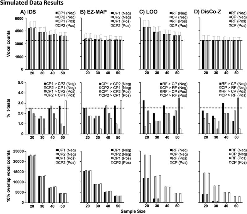
Simulations comparing biases in the independent sample (IDS; Column A), EZ-MAP (Column B), leave-one-out (LOO; Column C) and the DisCo-Z (Column D) algorithms. Data were initially derived from a normal distribution for both reference (RF) and comparison (CP) groups. Sample size (N) within each group is plotted on the x-axis. The first row presents the mean number of extreme voxels that were observed in each method. Error bars depict the average standard error of the mean across iterations, while the horizontal dotted line represents the empirically determined number of extrema for z > |2|. The second row depicts group-wise bias, measured by the percentage of t-tests that were statistically different (p < 0.05) between the RF and CP groups (LOO and DisCo-Z) or two CP (CP1 vs. CP2; IDS and EZ-MAP) groups, with the dotted line representing expected percentage of significant tests in a single tail. The third row presents the number of cases where 10% or more of the group present with extrema, with the decrease expected from binomial distribution theory in number of elements with greater than 10% overlap as a function of increasing N. Standard error of mean across iterations is too small to be visible in these graphs. Data are color-coded to reflect the number of extrema (Row 1), t-test results (Row 2), or overlap (Row 3) from the negative (Neg; black and light gray bars) and positive (Pos; dark gray and white bars) tails of the distribution. All methods eliminated global group-wise bias associated with unequal variances following z-transformations, whereas only algorithms based on an independent third sample eliminated spatial group-wise bias. Note that scales differ between all rows.
In contrast, the degree of spatial bias was strongly influenced by both the choice of z-transform method and sample size. As expected in more robust sample sizes, the number of elements with 10% or more overlap decreased as a function of increasing N across all methods. Both IDS and EZ-MAP methods utilize statistical moments derived from an independent reference group as the initial step in the z-transformation. Consequently, the transformed data initially resemble a t-distribution (i.e., heavier tails at lower sample sizes; Mayer et al. 2017), without evidence of group-wise bias in terms of how extrema are spatially distributed between CP1 and CP2 groups (Figure 1A and 1B third row).
Conversely, DisCo-Z and LOO are transformed using statistical moments from the RF group. This resulted in a pattern of spatial distribution bias (CP > RF) that increased as a function of N. Specifically, at N ≥ 40, spatial overlap in extrema was essentially non-existent in the RF group (Figure 1C&D; third row) while the number of extrema with spatial overlap in the CP group was similar to other methods that utilized independent samples (IDS and EZ-MAP) at similar sample sizes. To examine the primary determinant of these spatial biases, we examined differences between the first four statistical moments of the untransformed data (mean, SD, kurtosis, and skewness) resulting from both EZ-MAP (i.e., transformation based on independent third group) and DisCo-Z (i.e., transformation based on a dependent sample). Within each iteration, the difference in each statistical moment between the RF and CP groups (DisCo-Z) or between the CP1 and CP2 groups (EZ-MAP) was first calculated. Second, the signed differences for each moment were separately ranked by magnitude and assigned a percentile value. Finally, the average normalized frequency of elements that exhibited spatial overlap (at least 10% of sample) was plotted at bin intervals equal to every 5th percentile (Figure 2).
Fig. 2.
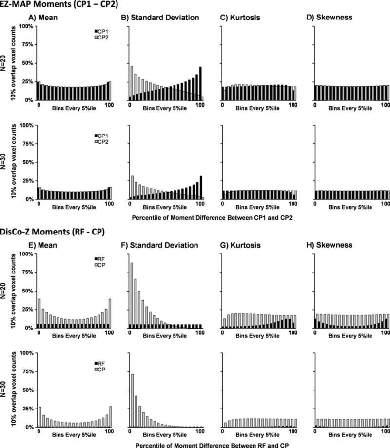
Simulations examining distribution of overlap given pre-transformation differences in statistical moments (mean [Panels A & E], standard deviation [Panels B & F], kurtosis [Panels C & G], and skewness [Panels D & H]) between the study reference (CP1; black) and comparison (CP2; grey) groups in EZ-MAP (Panels A–D) and reference (RF; black) and comparison (CP; grey) groups in DisCo-Z (Panels E-H) algorithms. Data were derived from a normal distribution for both groups at per group sample sizes (N) of 20 (first and third rows) and 30 (second and fourth rows) and assigned a bin based on the percentile value of the difference in the moments between untransformed group data across all tests. Data is shown as the mean number of voxels where 10% or more of group members presented with extrema in either the positive or negative tail of the distribution that were observed in each method and grouped as every 5th percentile between 0 and 100. Spatial bias in dependent-referencing methods appears to be due to difference in the first two statistical moments, with the majority of variance attributable to pre-normalization differences in standard deviation between the two groups.
As expected, the initial differences in statistical moments across CP1 and CP2 groups in the EZ-MAP method resulted in a relatively symmetrical pattern of spatial overlap in extrema reflected around the 50th percentile with no evidence of bias (Figure 2A–D). Moreover, the standard deviation, and to a lesser extent the mean, appeared to be the primary factor for determining whether individual elements were characterized by higher spatial overlap. Both skew and kurtosis did not appear to contribute bias, which is not unexpected given that data were derived from a normal distribution. Results from DisCo-Z indicated that differences in the standard deviation and the mean of the RF and CP groups were again the largest contributors for determining the extent of spatial overlap within individual elements (Figure 2E–F). Importantly, regardless of whether the CP or RF group exhibited a higher mean, the CP group always exhibited a higher percentage of spatial overlap in terms of extrema. Similarly, increased standard deviation in the CP relative to RF group also resulted in extremely high spatial overlap in terms of the pattern of extrema in the CP group. Thus, extrema in the CP group will always have a much higher probability of spatial overlap within the same element relative to extrema in the RF group even though the total number of extrema are equivalent.
Both of these phenomena can be easily understood based on the mathematical properties of a z-transform. Specifically, in cases where the CP and RF group means differ, the resulting z-transformed data for the CP group or groups will always be shifted away from zero, with a higher probability of outliers in either the positive or negative tail dependent on the direction of shift (see Figure 2E). Similarly, as expected a higher standard deviation within the CP relative to RF group results in a greater number of extrema (i.e., scatter) within z-transformed CP data (see Figure 2F). In contrast, higher standard deviation within the RF relative to CP group may reduce the magnitude of values in the z-transformed CP data as a result of division by a larger numerator (i.e., the RF group standard deviation) while having minimal impact on the scatter of z-transformed RF data.
Finally, we investigated whether the same group-wise bias in the spatial distribution of extrema present in simulations would exist when SSA methods were implemented with real data (Figure 3). Given the known correction to results using an independent sample from the preceding mathematical exploration of the z-transform equation (as demonstrated in Figure 2), analyses were limited to the DisCo-Z method. Results from a 2 × 2 [Group (RF vs. CP) × Tail (Positive vs. Negative) ANOVA at N = 30 per group (sample size equivalent in most imaging experiments) indicated a significantly higher number of voxels (F1,798=952.2; p<0.001) exhibiting spatial overlap of extrema for the CP (11,267.6±4,611.6) relative to RF group (3,642.0±1,778.1). In addition, the tail bias originally present in the raw count of suprathreshold voxels (Figure 3C) carried over to overlap count, with a significant main effect of tail (F1,798=44.9; p<0.001; Positive [8,319.3±6,809.4] > Negative [6,590.2±5,821.4]; p<0.001). Importantly, there were no differences between groups (p > 0.10) when the total number of extrema were simply summed as proposed in our original method (Mayer et al. 2014). Similar results were obtained at N = 20, 40 and 50 (see Figure 3C).
Fig. 3.
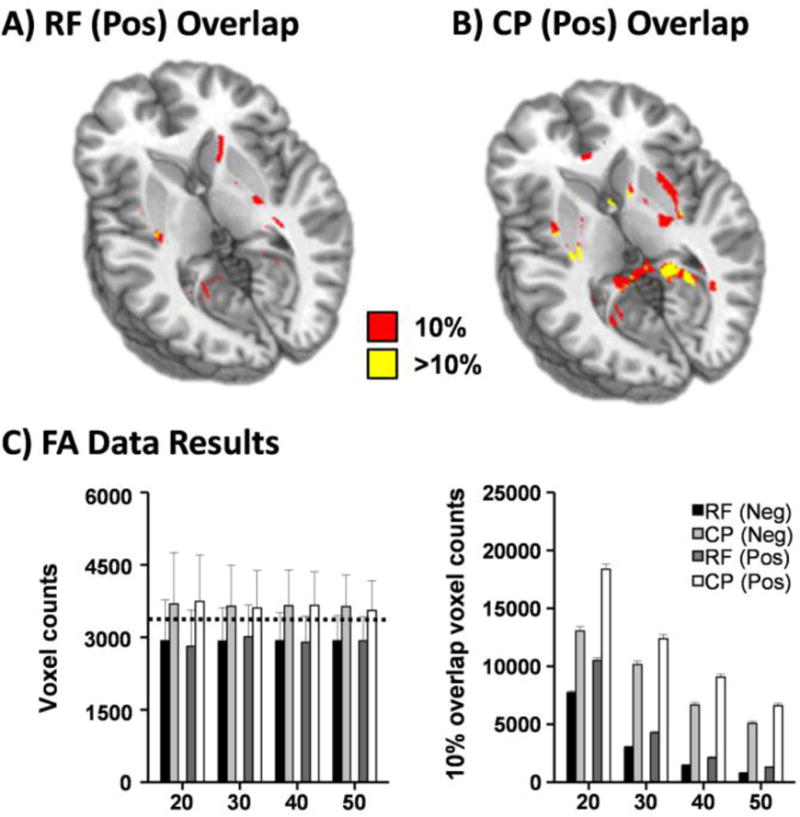
Fractional anisotropy data from 50 healthy controls were randomly sampled with replacement into reference (RF) and comparison (CP) groups across 400 iterations at samples sizes (N) from 20 to 50 by 10. The first row exhibits spatial results from an iteration representative of the average number of elements with 10% (red) or greater (yellow) overlap in the positive tail of RF (Panel A) and CP (Panel B) groups. Layout of Panel C is identical to Figure 1 (horizontal dotted lines, errors bars, etc.). While no global group-wise bias existed between the RF and CP groups, spatial bias (CP > RF) was present in the amount of overlap observed between individual z-transformed maps in both the negative (Neg; black and light gray bars) and positive (Pos; dark gray and white bars) tails of the distribution.
Conclusion
In summary, results from the current study suggest that inferences regarding the spatial distribution of SSA across multiple individuals following various z-transform methodologies are not statistically valid unless an independent third group is utilized for the initial z-transform. Although it has been repeatedly demonstrated that the LOO, IDS, EZ-MAP and DisCo-Z methods eliminate group-wise bias when SSA are summed across individuals (Bouix et al. 2013; Kim et al. 2013; Mayer et al. 2014; Mayer et al. 2017), recent attempts to quantify the number of individuals who exhibit SSA within the same voxel/region (Bouix et al. 2013; Hayes et al. 2015; Meier et al. 2016; Miller et al. 2016; Miller et al. 2016; Solmaz et al. 2017; Taber et al. 2015; White et al. 2013; White et al. 2015) or compute weighted statistics based on the proportion of individuals with extreme values (Ware et al. 2017) may be statistically flawed depending on the transform method utilized. Specifically, any SSA z-transform (e.g., LOO and DisCo-Z methods) that utilizes the first two statistical moments (mean and standard deviation) for both the transform itself as well as for subsequent comparison purposes will produce a bias in the spatial location of extrema. In contrast, methods that utilize statistical moments from an independent third group (e.g., EZ-MAP and IDS) do not produce a bias in the distribution of extrema.
This result is inevitable for both simulated and real data based on the mathematical formulation of z-score calculations. Large differences between the means of two samples will always result in a higher probability of extrema in the comparison sample due to the subtraction of the reference mean; only the sign (positive or negative) of the extrema will vary. Therefore, regardless of whether these differences in the mean are real or due to sampling error, the number of extrema will always be greater for the comparison group when the sample means differ. Conversely, whereas a large standard deviation (high scatter) in the comparison distribution increases the probability of extrema for the comparison group, a large standard deviation in the reference group differentially affects the probability of extrema in the reference (complex relationship) versus the comparison group (decreases magnitude of transformed values).
While deriving statistical moments from an independent third sample will alleviate the flaw inherent in transforming based on the reference sample, it is important to remember that, by design, SSA methods are meant to provide a location-independent summary of extrema load at the group level. The extension of the method for examining common spatial bias was not originally anticipated or intended, and is statistically similar to more standard group statistics (parametric or non-parametric) that explicitly test for differences in sample distributions. Importantly, the use of SSA methods to identify abnormal brain regions in a single subject and derive comparisons to clinical findings (e.g., SSA within motor tract resulting in hemiparesis) remains feasible if a large and representative sample size is utilized for derivation of normative data. In this way, SSA are similar to other blood and chemistry tests that are commonly utilized in medical settings.
Table 1 provides a brief summary of the four different z-score approaches for performing SSA. Foremost, all methods eliminate group-wise bias (i.e., differences between RF and CP groups) that has been shown to characterize the pothole method (Mayer et al. 2014; Watts et al. 2014). Second, both IDS and LOO incorrectly estimate the true number of extrema using traditional z-score thresholds across both normal and non-normal distributions (Mayer et al. 2017). Importantly, this over-estimation bias can either be fully (normal or kurtotic distributions) or partially (skewed data) addressed by approximating the distributional properties of transformed data using an approach like the DisCo-Z. Third, and most relevant to the current investigation, both IDS and EZ-MAP require an independent RF group. This can be costly and time-consuming for neuroimaging studies to implement (i.e., using the same imaging sequence), and potentially increases the risk of convenience sample usage rather than appropriate controls. The bootstrapping used in EZ-MAP is also computationally intensive. Conversely, the use of an independent sample means that neither IDS or EZ-MAP is affected by spatial bias when the investigatory goal is to test for the frequency of abnormalities in any given ROI/voxel. Thus, each approach has various strengths and weaknesses, some of which can be addressed depending on the desired goals of the study.
Table 1.
Cost-benefit profile of z-transform methods for SSA analyses.
| IDS | EZ-MAP | LOO | DisCo-Z | |
|---|---|---|---|---|
|
| ||||
| Eliminates Group-wise Bias | + + | + + | + + | + + |
| Eliminates Estimation Bias* (normal/kurtotic/skewed distributions) | − −/− −/− − | + +/+ +/+ | − −/− −/− − | + +/+ +/+ |
| Computational cost | + + | − − | + | + + |
| Additional financial/time cost (requires independent sample) | − − | − − | + + | + + |
| Eliminates Spatial Bias | + + | + + | − − | − − |
Notes: Number of positive/negative signs indicates degree of benefit/detriment for method.
Estimation bias can be reduced in IDS and LOO by a simple correction for distribution type as is done in DisCo-Z.
Acknowledgments
We would also like to thank Diana South and Catherine Smith for their assistance with data collection.
Funding. This work was supported by the National Institutes of Health (grant numbers 1R01MH101512-01A1 and 1R01NS098494-01A1) to A.R.M.. The funding agencies had no involvement in the study design, data collection, analyses, writing of the manuscript, or decisions related to submission for publication.
Footnotes
Compliance with Ethical Standards
Conflict of interest. Mr. Dodd reports no conflicts of interest. Mr. Ling reports no conflicts of interest. Dr. Bedrick reports no conflicts of interest. Dr. Meier reports no conflicts of interest. Dr. Mayer reports no conflicts of interest.
Ethical approval. All procedures performed in studies involving human participants were in accordance with the ethical standards of the institutional and/or national research committee and with the 1964 Helsinki declaration and its later amendments or comparable ethical standards.
Informed consent. Informed consent was obtained from all individual participants included in the study.
References
- Bouix S, Pasternak O, Rathi Y, Pelavin PE, Zafonte R, Shenton ME. Increased gray matter diffusion anisotropy in patients with persistent post-concussive symptoms following mild traumatic brain injury. PLoS One. 2013;8(6):e66205. doi: 10.1371/journal.pone.0066205. [DOI] [PMC free article] [PubMed] [Google Scholar]
- Hayes JP, Miller DR, Lafleche G, Salat DH, Verfaellie M. The nature of white matter abnormalities in blast-related mild traumatic brain injury. Neuroimage Clin. 2015;8:148–156. doi: 10.1016/j.nicl.2015.04.001. [DOI] [PMC free article] [PubMed] [Google Scholar]
- Kim N, Branch CA, Kim M, Lipton ML. Whole brain approaches for identification of microstructural abnormalities in individual patients: Comparison of techniques applied to mild traumatic brain injury. PLoS ONE. 2013;8(3):e59382. doi: 10.1371/journal.pone.0059382. [DOI] [PMC free article] [PubMed] [Google Scholar]
- Mayer AR, Bedrick EJ, Ling JM, Toulouse T, Dodd A. Methods for identifying subject-specific abnormalities in neuroimaging data. Hum Brain Mapp. 2014;35(11):5457–5470. doi: 10.1002/hbm.22563. [DOI] [PMC free article] [PubMed] [Google Scholar]
- Mayer AR, Dodd AB, Ling JM, Wertz CJ, Shaff NA, Bedrick EJ, et al. An evaluation of Z-transform algorithms for identifying subject-specific abnormalities in neuroimaging data. Brain Imaging Behav. 2017 doi: 10.1007/s11682-017-9702-2. [DOI] [PMC free article] [PubMed] [Google Scholar]
- Meier TB, Bergamino M, Bellgowan PS, Teague TK, Ling JM, Jeromin A, et al. Longitudinal assessment of white matter abnormalities following sports–related concussion. Human Brain Mapping. 2016;37(2):833–845. doi: 10.1002/hbm.23072. [DOI] [PMC free article] [PubMed] [Google Scholar]
- Miller DR, Hayes JP, Lafleche G, Salat DH, Verfaellie M. White matter abnormalities are associated with chronic postconcussion symptoms in blast-related mild traumatic brain injury. Hum Brain Mapp. 2016;37(1):220–229. doi: 10.1002/hbm.23022. [DOI] [PMC free article] [PubMed] [Google Scholar]
- Miller DR, Hayes JP, Lafleche G, Salat DH, Verfaellie M. White matter abnormalities are associated with overall cognitive status in blast-related mTBI. Brain Imaging Behav. 2016 doi: 10.1007/s11682-016-9593-7. [DOI] [PMC free article] [PubMed] [Google Scholar]
- Pasternak O, Koerte IK, Bouix S, Fredman E, Sasaki T, Mayinger M, et al. Hockey Concussion Education Project, Part 2. Microstructural white matter alterations in acutely concussed ice hockey players: a longitudinal free-water MRI study. J Neurosurg. 2014;120(4):873–881. doi: 10.3171/2013.12.JNS132090. [DOI] [PMC free article] [PubMed] [Google Scholar]
- Seghier ML, Price CJ. Visualising inter-subject variability in fMRI using threshold-weighted overlap maps. Sci Rep. 2016;6:20170. doi: 10.1038/srep20170. [DOI] [PMC free article] [PubMed] [Google Scholar]
- Solmaz B, Tunc B, Parker D, Whyte J, Hart T, Rabinowitz A, et al. Assessing connectivity related injury burden in diffuse traumatic brain injury. Hum Brain Mapp. 2017 doi: 10.1002/hbm.23561. [DOI] [PMC free article] [PubMed] [Google Scholar]
- Taber KH, Hurley RA, Haswell CC, Rowland JA, Hurt SD, Lamar CD, et al. White matter compromise in veterans exposed to primary blast forces. J Head Trauma Rehabil. 2015;30(1):E15–E25. doi: 10.1097/HTR.0000000000000030. [DOI] [PMC free article] [PubMed] [Google Scholar]
- Ware JB, Hart T, Whyte J, Rabinowitz A, Detre JA, Kim J. Inter-subject variability of axonal injury in diffuse traumatic brain injury. J Neurotrauma. 2017 doi: 10.1089/neu.2016.4817. [DOI] [PMC free article] [PubMed] [Google Scholar]
- Watts R, Thomas A, Filippi CG, Nickerson JP, Freeman K. Potholes and molehills: Bias in the diagnostic performance of diffusion-tensor imaging in concussion. Radiology. 2014;272(1):217–223. doi: 10.1148/radiol.14131856. [DOI] [PMC free article] [PubMed] [Google Scholar]
- White T, Ehrlich S, Ho BC, Manoach DS, Caprihan A, Schulz SC, et al. Spatial characteristics of white matter abnormalities in schizophrenia. Schizophr Bull. 2013;39(5):1077–1086. doi: 10.1093/schbul/sbs106. [DOI] [PMC free article] [PubMed] [Google Scholar]
- White T, Langen C, Schmidt M, Hough M, James A. Comparative neuropsychiatry: white matter abnormalities in children and adolescents with schizophrenia, bipolar affective disorder, and obsessive-compulsive disorder. Eur Psychiatry. 2015;30(2):205–213. doi: 10.1016/j.eurpsy.2014.10.003. [DOI] [PubMed] [Google Scholar]