Analytical model of electro-hydrodynamic flow in corona discharge

Abstract

We present an analytical model for electro-hydrodynamic flow that describes the relationship between the corona voltage, electric field, and ion charge density. The interaction between the accelerated ions and the neutral gas molecules is modeled as an external body force in the Navier-Stokes equation. The gas flow characteristics are solved from conservation principles with spectral methods. This multiphysics model is shown to match experimental data for a point-to-ring corona configuration, shedding new insights into mass, charge, and momentum transport phenomena, and can be readily implemented in any numerical simulation.

I. INTRODUCTION

Corona discharge generates a flow of ions in a strong electric field between two electrodes; the high-velocity ions transfer their kinetic energy to the neutral air molecules by collisions that accelerate the gas in the direction of ion drift. This electrohydrodynamic (EHD) flow propulsion phenomenon, also referred to in the literature as ionic wind, is used in many practical applications, such as convective cooling,^1–6 electrostatic precipitators (ESPs),^7–10 plasma assisted combustion,¹¹ airflow control,^12,13 and as a turbulent boundary layer actuator.¹⁴ The ions' acceleration in the electric field and their interaction with the neutral molecules in the ion drift region can be modeled as an external force term (Coulomb force) in the Navier-Stokes equation (NSE). A two-part model is required: (i) the description of the ion motion in the electrical field and (ii) the effect of the ion drift on the neutral gas in the flow acceleration region.

The voltage-current $(\phi -I)$ relation during the corona discharge characterizes the ion motion between the electrodes globally. This phenomenon has been studied since the early 20th century. The classic $(\phi -I)$ relationship was derived by Townsend¹⁵ in 1914 and validated for a coaxial corona configuration. The quadratic relationship has been validated for various corona geometries, such as point-to-pot,¹⁶ point-to-plate,¹⁷ and point-to-ring.¹⁸ In a point-to ring corona, Giubbilini also demonstrated that the ion current is inversely proportional to the point-to-ring distance.¹⁸

Some recent studies modify Townsend's quadratic relationship to better describe the $(\phi -I)$ relationship for different electrode configurations, e.g., point-to-plate,^19,20 point-to-grid,²¹ point-to-cylinder,²² sphere-to-plane,²³ coaxial cylinders,^24,25 wire-cylinder-plate,^26–28 point-to-ring,^18,29,30 parallel electrodes,³¹ multi-electrodes,³² and non-uniform electric fields.³³ In propulsion studies, the electrostatic force has been modeled using various hydrodynamic terms, such as body forces³⁴ or pressure (drag).⁷ Typically, the ionic wind velocity is experimentally described as a function of the corona anode voltage.^30,35–37 The previous experimental study of point-to-ring geometry investigated external EHD flow;³⁰ the internal EHD flow can provide more consistent measurement and achieve higher velocities due to more efficient axial flow acceleration. The existing literature does not provide a first-principles approach to modeling the EHD effect for an arbitrary electrode configuration.

In this work, we develop an analytical model for corona-driven EHD flow and validate the model against the experimental measurements in air. The conceptual representation of the EHD system includes (i) gas ionization region, (ii) flow acceleration region where unipolar ion motion in the gas medium acts as a body force accelerating the flow, and (iii) momentum conservation region dominated by the inertial and viscous terms of the NSE. These regions do not necessarily have clear boundaries; however, they can be characterized based on the flow non-dimensional parameters dominant in each of them. The model presented in this paper addresses the flow acceleration behavior resulting from ion collisions with neutral air molecules in the ion drift region. During the development, we first obtain the relationship between the electrical properties of the EHD flow, such as corona voltage $\phi$, electric field $\mathbf{E}$, and charge density ${\rho }_c$ for planar, cylindrical, and spherical coordinates. Then, the EHD velocity profiles are solved numerically using a Chebyshev spectral method. Finally, the analytical model is compared with the experimental data for a point-to-ring corona in an internal pipe flow configuration.

II. EXPERIMENTAL SETUP

Experimental measurements for point-to-ring corona are used to inspire model development and for its validation. In the experiments, the two main relationships sought after are voltage-current $(\phi -I)$, obtained from the anode and cathode, and voltage-velocity $(\phi -u)$, based on the velocity measurements at the exit of the device. Figure 1 shows the experimental setup. The EHD flow is generated between a charged needle and a grounded ring. The anode needle is a 0.5 mm thick tungsten wire with a radius of curvature at the tip of 1 μm (measured by optical microscopy). It was previously shown that the sharpness of the needle affects the corona discharge at low voltages.³⁸ To ensure that the needle does not degrade over time, the tip of the needle was inspected routinely. The metal ring is a 1.58 mm thick solid solder with an inner radius of 10 mm. The enclosure is 3D printed with the polylactic acid filament. The air gap between the needle and the ring (L) was varied from 3 mm to 7 mm using 3D printed spacers. A high voltage positive DC power supply (Bertan 205B-20R) is used to create the electric potential between the needle and the ring. The cathode current was measured on the cathode based on a voltage drop across a 1 MΩ resistor.

FIG. 1.

Schematic of the experimental setup and EHD flow generator; a high voltage is applied between the corona anode needle and the ion collecting cathode ring.

The EHD experiment was operated in the positive corona mode in a temperature range of 22–25 °C, a relative humidity of 23%–25%, and ambient pressure. For each anode-cathode distance, the voltage was increased from 4 kV (when the outlet velocity is measurable) to ∼10 kV (when the arc discharge occurs). Constant current hot-wire anemometry was used to measure the flow velocity profile. A TSI 1213‐20 probe connected to the anemometer (AA-1005) was positioned at the outlet of the device. The anemometer probe is calibrated in the range of 0.2 m/s–8 m/s according to standard procedures.³⁹ The experimental setup was mounted on an optical table with the anemometer probe attached to the three-dimensional optical stage to provide space-resolved measurements. All components and the probe are grounded. The data from the anemometer are sampled at a frequency of 10 kHz using a data acquisition system (myRIO-1900) for a sampling time of 30 s. Each experimental condition is tested at least five times to obtain independent statistical samples. For each distance L, the applied high voltage increases from 4 kV, where the outlet velocity is measurable to around 10 kV or at the onset of the arc discharge.

III. ANALYTICAL MODEL DEVELOPMENT

The analytical expression for $(\phi -I)$ and $(\phi -u)$ relationships is derived for the steady-state conditions in the planar, cylindrical, and spherical coordinates.

A. Voltage-current relationship

The density ${\rho }_k$ of the charged species $k$ follows the conservation equation^22,27,28,40

$$\frac{\partial {\rho }_k}{\partial t}+\nabla ·\left[\left(\mathbf{u}+{\mu }_{bk}\mathbf{E}\right){\rho }_k-D_k\nabla {\rho }_k\right]={\omega }_k,$$ (1)

where $\mathbf{u}$ is the velocity vector of the bulk flow, $\mathbf{E}$ is the electric field vector, ${\mu }_{bk}$ and $D_k$ are mobility and diffusivity of each charged species $k$, and ${\omega }_k$ is the production rate of species $k$. The ionization is often conceptualized as two processes: (i) ionization process where ion species are generated and (ii) reattachment processes where charges recombine. Multiple analytical and numerical models for production rate ${\omega }_k$ have been presented in the literature; the rate is often modeled as a function of species density, mobility with derived ionization, and recombination coefficients.^20,22,28,40

In the context of the EHD flow model development, two observations on the ionization region are important. First, the ionization process is assumed to occur only in the region where the electric field strength is greater than a threshold value $E_i\approx 3\times {10}^6\hspace{0.17em}\mathrm{V}/\mathrm{m}$;^17,41 thus, the ionization is limited to a small region near the anode. The ionization region length scale—b can be approximated by $\frac{{\phi }_0}{E_i}$, where ${\phi }_0$ is the anode voltage.^40,42 Second, the positive and negative species within the ionization zone travel in opposite directions: positive ions move towards the cathode; negative ions and electrons—towards the anode. The total momentum exerted on the gas neutral molecules within the ionization region is negligible compared to that in the unipolar drift region; thus, the detailed description of the ionization region is not necessary for this model to work, as long as bulk properties related to energy transfer can be obtained. In order to relate the electrical power to the kinetic energy in the flow, the source term needs to be evaluated. In this work, we estimate the energy input based on the experimental measurements of the corona current. We assume that flow acceleration takes place in the acceleration region only within the ion drift region where the net charge density ${\rho }_c=\sum _k{\rho }_k$ participates in electric to kinetic energy conversion through ion/neutral molecule collisions.

The effective continuity equation for the charge density in the drift region is

$$\frac{\partial {\rho }_c}{\partial t}+\nabla ·\left[\left(\mathbf{u}+{\mu }_b\mathbf{E}\right){\rho }_c-D_c\nabla {\rho }_c\right]=0,$$ (2)

where ${\rho }_c$ is the charge density, $\mathbf{u}$ is the velocity vector of the bulk flow, $\mathbf{E}$ is the electric field vector, ${\mu }_b$ is the effective ion mobility, which is approximated as a constant ($2.0\times {10}^{-4}\hspace{0.17em}{\mathrm{m}}^2/\text{Vs}$) at atmospheric pressure and room temperature (300 K),^5,9,41,43,44 (this constant is likely to have different values for negative corona or corona in other gases), and $D_c$ is the ion diffusivity, described by the electrical mobility equation

$$D_c=\frac{{\mu }_b{k}_{B}T}{q},$$ (3)

where $k_B$ is Boltzmann's constant, $T$ is the absolute temperature, and $q$ is the electrical charge of an ion, which is equal to the elementary charge in this case.

The electric field satisfies Maxwell's equation

$$\nabla ·\mathbf{E}=\frac{{\rho }_c}{\epsilon },$$ (4)

where $\epsilon$ is the air permittivity close to the permittivity of free space.

Since the ion drift velocity is considerably greater than the velocity of the resulting EHD flow, the ion motion equation can be assumed to be quasi-steady

$$\nabla ·\left[\left(\mathbf{u}+{\mu }_b\mathbf{E}\right){\rho }_c-D_c\nabla {\rho }_c\right]=0.$$ (5)

To estimate the effect of the charge diffusion, consider the Sherwood number for ionic transport in the presence of strong external electric field

$$Sh=\frac{\mathbf{u}+{\mu }_b\mathbf{E}}{\left(\frac{D_e}{L_{\mathrm{d}}}\right)}\approx \frac{\left|\mathbf{E}\right|Lq}{k_{B}T}\sim O\left({10}^4\right),$$ (6)

where $L_{\mathrm{d}}$ is the diffusion length scale. The diffusion term can be neglected, further reducing the charge continuity equation to

$$\nabla ·\left[\left(\mathbf{u}+{\mu }_b\mathbf{E}\right){\rho }_c\right]=0,$$ (7)

and since $\frac{\left|\mathbf{u}\right|}{\left|{\mu }_b\mathbf{E}\right|}=\frac{O(1)}{O(100)}=O({10}^{-2})$ in air discharge,^2,5,9,41 the continuity equation for ions is reduced to

$$\nabla ·\left[{\mu }_b{\rho }_c\mathbf{E}\right]=0,$$ (8)

where ${\mu }_b{\rho }_c\mathbf{E}=\mathbf{J}$; $\mathbf{J}$ is the current flux $[\mathrm{A}/{\mathrm{m}}^2]$. Combining with Eq. (4), the ion transport equation can be written as

$$\frac{{\mu }_b}{\epsilon }{\rho }_c^2-{\mu }_b\nabla \phi \nabla {\rho }_c=0.$$ (9)

Note that Eq. (9) is the same as Eq. (5) in Sigmond¹⁷ if ${\rho }_c$ is substituted by $-\epsilon {\nabla }^2\phi$. Here, the derivation for spherical coordinates is presented. Derivations for Cartesian and cylindrical coordinates are similar and provided in the supplementary material. Dividing both sides of Eq. (9) by ${\mu }_b$ and rearranging gives

$$\nabla \phi =\frac{{\rho }_c^2}{\epsilon \nabla {\rho }_c}.$$ (10)

Taking the divergence on both sides and applying Maxwell's equation [Eq. (4)] provides

$${\nabla }^2\phi =-\frac{{\rho }_c}{\epsilon }=\nabla ·\left(\frac{{\rho }_c^2}{\epsilon \nabla {\rho }_c}\right)=\frac{1}{r^2}\frac{d}{dr}\left(\frac{r^2{\rho }_c^2}{\epsilon \frac{d{\rho }_c}{dr}}\right)=\frac{1}{r^2}\frac{\left(2r^2{\rho }_c\frac{d{\rho }_c}{dr}+2r{\rho }_c^2\right)\left(\epsilon \frac{d{\rho }_c}{dr}\right)-r^2{\rho }_c^2\left(\epsilon \frac{d^2{\rho }_c}{d{r}^2}\right)}{{\left(\epsilon \frac{d{\rho }_c}{dr}\right)}^2}.$$ (11)

Rearranging, we have

$$r{\rho }_c\left(\frac{d^2{\rho }_c}{d{r}^2}\right)=r{\left(\frac{d{\rho }_c}{dr}\right)}^2+\left(2r\frac{d{\rho }_c}{dr}+2{\rho }_c\right)\left(\frac{d{\rho }_c}{dr}\right).$$ (12)

One possible solution has the form

$${\rho }_c={\rho }_0{r}^n.$$ (13)

Substituting it into Eq. (12) gives

$$n\left(n-1\right)r^{2n-1}=n^2{r}^{2n-1}+\left(2n{r}^n+2r^n\right)n{r}^{n-1},$$ (14)

$$n\left(n-1\right)=n^2+\left(2n+2\right)n;$$ (15)

therefore, $n=-3/2$ and ${\rho }_c={\rho }_0{r}^{-3/2}$, and the substitution into Eq. (9) gives

$$E=-\frac{d}{dr}\phi =-\frac{{\rho }_c^2}{\left(\epsilon \frac{d{\rho }_c}{dr}\right)}=\frac{2{\rho }_0}{3\epsilon }{r}^{-1/2},$$ (16)

$$d\phi =-\frac{2{\rho }_0}{3\epsilon }{r}^{-1/2}dr,$$ (17)

integrating both sides

$$\phi -{\phi }_0=-\frac{4{\rho }_0}{3\epsilon }{r}^{1/2}.$$ (18)

Table I shows the solutions for this nonlinear differential equation in different coordinate systems; $r$ is the distance from the anode (mm).

TABLE I.

Solutions for the ion transport equation in one dimensional Cartesian, cylindrical coordinates, and spherical coordinates.

Variables	Planar coordinates	Cylindrical coordinates	Spherical coordinates
${\rho }_c$	${\rho }_c={\rho }_0{(r+r_0)}^{-1/2}$	${\rho }_c={\rho }_0{r}^{-1}$	${\rho }_c={\rho }_0{r}^{-3/2}$
$E=\left|\mathbf{E}\right|$	$E=\frac{2{\rho }_0}{\epsilon }{(r+r_0)}^{1/2}$	$E=\frac{{\rho }_0}{\epsilon }$	$E=\frac{2{\rho }_0}{3\epsilon }{r}^{-1/2}$
$\phi$	${\phi }_0-\frac{4{\rho }_0}{3\epsilon }{(r+r_0)}^{3/2}$	${\phi }_0-\frac{{\rho }_0}{\epsilon }r$	${\phi }_0-\frac{4{\rho }_0}{3\epsilon }{r}^{1/2}$
${\rho }_0$	$\frac{C}{m^3}(m{m}^{1/2})$	$\frac{C}{m^3}(mm)$	$\frac{C}{m^3}(m{m}^{3/2})$

Here, ${\phi }_0$ is the anode voltage and ${\rho }_0$ is a dimensional parameter [which is not necessarily a constant and for the fixed ionization volume may vary with corona voltage, see Eq. (24)]; the units depend on the coordinate system. The integration constant only appears in the voltage $\phi$ since Eq. (9) only depends on the gradient of $\phi$. Integration constant $r_0$ appears in planar coordinates. The solution for planar coordinates is exactly the same as previous research that uses a non-diffusive charge assumption.^45,46 For a point-to-ring geometry, the ionization and drift regions are best approximated as spherical sectors with a radius $r$ and angle $\beta$ determined by the position of the corona needle, as shown in Fig. 2

$$\text{cos}\hspace{0.17em}\beta =\frac{L}{\sqrt{L^2+R^2}},$$ (19)

where $L$ is the distance between the needle tip to the center of the cathode and $R$ is the radius of the cathode ring.

FIG. 2.

Diagram of the point-to-ring corona system with current flux distribution.

The ion current flux magnitude between the needle and the ring is

$$J=\left|\mathbf{J}\right|={\mu }_b{\rho }_{c}E=\frac{2{\mu }_b{\rho }_0^2}{3\epsilon r^2}.$$ (20)

Equation (20) shows that $J\propto r^{-2}$. The current flux distribution is given as

$$\frac{J}{J_o}={\left(\frac{r{(\text{cos}\hspace{0.17em}\theta )}^{-1}}{r}\right)}^{-2}={\text{cos}}^2\hspace{0.17em}\theta ,$$ (21)

where $J_o$ is the maximum current flux distribution and $\theta$ is the solid angle of the discharge, $\theta \in [0,\beta ]$. Considering the axial component of current flux, $\theta =0$

$$J_a=J\hspace{0.17em}\text{cos}\hspace{0.17em}\theta =J_o\hspace{0.17em}{\text{cos}}^3\hspace{0.17em}\theta ,$$ (22)

where $J_a$ is the current flux in the axial direction.

To define the conditions in the acceleration region, consider $r_{cr}$, the characteristic length scale of the flow acceleration region, as the radius of a spherical surface with the electric potential equal to ${\phi }_{cr}$ (defined as the onset voltage of the corona, similar to the definition by Townsend¹⁵) The current flux at the critical surface can be written as

$$J_{cr}=\frac{2{\mu }_b{\rho }_0^2}{3\epsilon r_{cr}^2}.$$ (23)

In spherical coordinates for the point-to-ring geometry

$${\rho }_0=\frac{3\epsilon }{4r_{cr}^{1/2}}\left({\phi }_0-{\phi }_{cr}\right).$$ (24)

Therefore,

$$J_{cr}=\frac{3{\mu }_b\epsilon }{8r_{cr}^3}{\left({\phi }_0-{\phi }_{cr}\right)}^2.$$ (25)

Due to the conservation of current flux, the corona current can be found by integrating the current flux over the spherical dome

$$I=\underset{cr}{\int }{J}_{cr}dA=J_{cr}{A}_{cr}=\frac{3\pi {\mu }_b\epsilon }{4r_{cr}}\left(1-\frac{L}{\sqrt{L^2+R^2}}\right){\left({\phi }_0-{\phi }_{cr}\right)}^2.$$ (26)

Equation (26) is similar to Townsend's quadratic relationship for the coaxial-cylinder electrode configuration $I=C_{cyl}{\phi }_0({\phi }_0-{\phi }_c)$, where $C_{cyl}=\frac{8\pi {\mu }_b\epsilon }{R^2\hspace{0.17em}\text{ln}\hspace{0.17em}(R/r)}$ is a geometrically dependent constant.¹⁵ For cylindrical coordinates, replacing $E=\frac{{\rho }_0}{\epsilon }$ by $E=\frac{{\phi }_0}{R\hspace{0.17em}\text{ln}\hspace{0.17em}R/r}$ and for $r_{cr}=R/4$, the $\phi -I$ relation is identical to that of Townsend. Equation (26) is also similar to the one derived by Sigmond for a space-charge saturated point-to-plate corona discharge using time-dependent analysis,¹⁷ where $I=2{\mu }_b\epsilon {\phi }^2/L$. The $\phi -I$ relationship derived in this work is more general than particular formulations presented in Refs. 15 and 17. However, for a specific geometry, the values of ${\phi }_{cr}$ and the corresponding length scale, $r_{cr}$, need to be determined experimentally or additional assumptions need to be made. Once the $\phi -I$ relation is defined, the EHD velocity can be computed. Recently, Monrolin et al.⁴⁷ derived an analytical expression for onset voltage of co-axial positive corona discharge (cylindrical coordinates) using the asymptotic method proposed by Durbin and Turyn.⁴⁸ The onset voltage was modeled as ${\phi }_{cr}=r_{em}{E}_{cr}\hspace{0.17em}\text{ln}\hspace{0.17em}(r_{co}/r_{em})$, where $r_{em}$ and $r_{co}$ are the radius of the emitter (inner cylinder) and collector (outer cylinder), respectively; $E_{cr}$ is a constant which depends on the geometry and gas properties. This formulation can be used for determining the ionization region properties in cylindrical coordinates, such as $r_{cr}$ and $b$ for relations shown in Table I. However, unlike the co-axial case, the electric field is not uniform in the point-to-ring corona discharge. Therefore, the onset voltage expression may have a different form and the relation between the ionization region properties and onset voltage may also be different.

B. Voltage-velocity relationship

The EHD flow induced by point-to-ring discharge can be divided into three regions: ionization zone, acceleration region, and momentum conservation region. The ionization region does not have a significant effect on the momentum exchange between the charged species and neutral molecule as the momentum exerted by negative and positive species is assumed to be balanced, which is a well-accepted approximation for EHD flows.^{2–5,41,44,49–52} Electro-kinetic phenomena such as plasma waves and streaming may have minor effects on the EHD flow development; however, in this study these second order effects are not considered. Non-dimensional analysis shows that the acceleration region can be defined by the high ion concentration and high electric field strength.⁴¹ The momentum conservation region is the part of the domain where electric force is balanced or overcome by viscous forces near the walls. Figure 3 illustrates the relative positions of the ionization zone, EHD acceleration region, and EHD momentum dissipation region. The ion drift zone includes both the EHD acceleration region and the EHD momentum dissipation region,^20,22,28,40 as shown in Fig. 3. The ion drift zone is the region where the efficient charge density and the electric field are both non-zero. The size of the ion drift zone only depends on the geometry of the electrode configuration.

FIG. 3.

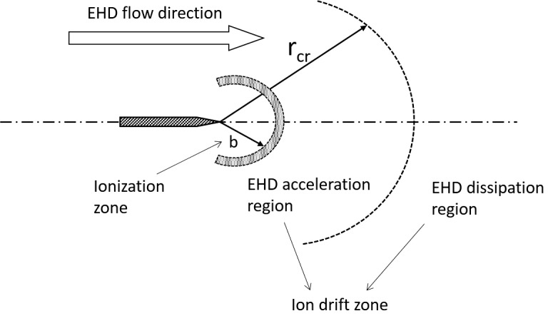
Diagram of the relations among the ionization zone, EHD acceleration region, and EHD dissipation region of a point-to-ring corona system.

The steady-state energy equation for a constant area pipe can be written as

$$S{E}_{\mathit{\text{inlet}}}=S{E}_{out}+S{E}_e,$$ (27)

where $S{E}_e$ is the energy gained from the electric force ($SE$ denotes specific energy with a unit of J/kg), which can be written as

$$S{E}_e=\frac{\int {\rho }_{c}Edr}{\rho }=\frac{\int Jdr}{\rho {\mu }_b}=\frac{3\epsilon }{8\rho r_{cr}}{\left({\phi }_0-{\phi }_{cr}\right)}^2\underset{b}{\overset{r_c}{\int }}{r}^{-2}dr,$$ (28)

where $\rho$ is the mean density of the flow. Since both the inlet and outlet are at atmospheric pressure and the flow is in the direction of the electric field line, the velocity on the axis of the cylindrical pipe is

$$u_{\max }=\sqrt{2S{E}_e}={\left[\frac{3\epsilon }{4\rho r_{cr}}\underset{b}{\overset{r_{cr}}{\int }}{r}^{-2}dr\right]}^{1/2}\left({\phi }_0-{\phi }_{cr}\right).$$ (29)

The force is acting only on the gas downstream of the ionization region; thus, the lower integration limit is set to the ionization zone boundary, b

$$u_{\max }={\left[\frac{3\epsilon }{4\rho r_{cr}}\underset{b}{\overset{r_{cr}}{\int }}{r}^{-2}dr\right]}^{1/2}\left({\phi }_0-{\phi }_{cr}\right).$$ (30)

C. Velocity profile

The velocity profile in a cylindrical pipe for the point-to-ring configuration is obtained under the assumption that the electric force results only in axial flow acceleration. Viscous drag is balanced by the electric force on the ions. In cylindrical coordinates

$$\mu \left(\frac{{\partial }^2{u}_a}{\partial r^2}+\frac{1}{r}\frac{\partial u_a}{\partial r}\right)=-{\rho }_c{E}_a=-\frac{J_a}{{\mu }_b},$$ (31)

$$\text{cos}\hspace{0.17em}\theta =\frac{L}{\sqrt{L^2+r^2}},$$ (32)

where subscript $a$ denotes the axial component of the vectors. Substituting Eqs. (22) and (32) in Eq. (31) and rearranging the terms results in the following ordinary differential equation (ODE):

$$r\frac{{\partial }^2{u}_a}{\partial r^2}+\frac{\partial u_a}{\partial r}=-\frac{J_0{L}^3}{\mu {\mu }_b}\left[\frac{r}{{\left(r^2+L^2\right)}^{3/2}}\right].$$ (33)

The ordinary differential equation is solved numerically using Chebyshev polynomial approximation with the MATLAB package chebfun.^53–56 Neumann boundary conditions (zero-flux) are used at the axis and the non-slip boundary condition (zero-velocity) at the wall. The Chebyshev differential matrices for first and second derivatives are constructed to satisfy the boundary conditions.⁵⁵

IV. RESULTS AND DISCUSSION

The experimental data are compared with the model in Fig. 4(a), which shows the comparison of the corona current-voltage relationship. The $I/\phi$ vs. $\phi$ trends are different from the previously reported linear trends^18,30 for the external flow in the point-to-ring corona configuration. The nonlinearity in the analytical model comes from the ${\phi }_{\text{cr}}/{\phi }_0$ term, as seen in Eq. (26). However, for the high values of ${\phi }_0$ where most previously reported data were collected, the linear curve fit may have been adequate. These trends can be used to evaluate boundary conditions for modeling of the acceleration region. One approach is to evaluate the critical properties of the acceleration zone at the onset of corona discharge, as the anode voltage approaches the critical voltage, i.e., ${\phi }_0\to {\phi }_{cr}$, the ${\phi }_{cr}=2\hspace{0.17em}\mathrm{k}\mathrm{V}$ based on the x-axis. At this condition $r_{cr}\to b$ and EHD flow velocity is negligible. As the corona voltage increases, the size of the acceleration zone $r_{cr}$ and the field intensity increase non-linearly. The current and velocity data in this non-linear region fluctuate, resulting in $r_{cr}$ variations. In the linear region, observed at the higher corona voltages and in previous reports,^18,30 both the current values and the EHD velocities were stable indicating well-established ionization and acceleration regions. As in previous work,^17,18,30 the acceleration region dimensions are considered constant for a given electrode configuration, i.e., linearly dependent on $L$. The best fit for the data in the presented point-to-ring internal EHD flow is obtained when $r_{cr}=3+0.5(L-3)$. This relationship is likely to change for a different electrode configuration. The dimensions of the ionization boundary can be approximated as $\frac{{\phi }_0}{E_i}$.^40,42 In the linear regime, we assume $E_i=\alpha E_{cr}$, where $E_{cr}$ is the critical electric field strength at $r_{cr}$ and $\alpha$ is a scaling factor. Since for ${\phi }_0\to {\phi }_{cr}$ (no ionization occurs) $b\to 0$, we consider the following relationship:

$$b=\frac{{\phi }_0-{\phi }_{cr}}{\alpha E_{cr}}=\frac{\frac{4{\rho }_0}{3\epsilon }{r}_{cr}^{1/2}}{\frac{2\alpha {\rho }_0}{3\epsilon }{r}_{cr}^{-1/2}}=\frac{2}{\alpha }{r}_{cr}.$$ (34)

FIG. 4.

Current-voltage $(\phi -I)$ and voltage-velocity $(\phi -u)$ for the experimental data and the analytical solution.

In this work, the evaluation of $\alpha$ is based on experimental data, and the best agreement with data is observed for $\alpha =8$.

Figure 4(b) shows the comparison of the voltage-velocity $(\phi -u)$ data against the analytical solution for a range of $L$ = 3–7 mm and $\phi$ = 4–10 kV. The trends agree with the previously reported linear dependence between the maximum velocity and corona voltage observed for the point-to-ring corona configurations³⁰ and planar electric field ion generator.⁵⁷ The analytical solution uses $b=r_{cr}/4$ as the ionization zone boundary for the integration of Eq. (30). Analytical solutions for corona current and maximum velocity are in very good agreement with the experimental data over the entire range of geometrical and operational parameters of the EHD source.

Figure 5 shows the velocity profiles at the exit of the point-to-ring EHD flow generator. The velocity profile has some similarities with a momentum point-source jet, with a maximum at the centerline and a steep decrease towards the domain boundaries. Figure 5(a) shows the velocity profile plotted for two voltage values, keeping $L$ constant; the velocity increases with the increase in the corona voltage. Figure 5(b) shows the velocity increase for lower values of L at a fixed corona voltage. Both trends can be explained by the increase in the EHD force driving the flow based on the higher electric field intensity ($E=\varphi /L$).

FIG. 5.

Comparison between the analytical and the experimental velocity profiles at the outlet of the EHD generator; (a) corona voltages are 5 kV and 7 kV, fixed L = 3 mm; (b) electrode gaps are 3 mm and 7 mm, corona voltage is constant (7 kV).

Both the analytical solution and the experimental results show velocity profiles with a very distinct peak at the axis of the coaxial configuration, consistent with the localized electro-hydrodynamic force at the tip of the needle electrode. The velocity profiles then decay quickly over a short radial distance (of the order of the ionization zone width, r_cr/4) with asymptotic decay towards the edge of the domain, consistent with entrainment in a confined flow environment. The comparison between the analytical solution and the data is excellent at the centerline; the velocity decays approaching the wall are not captured well by the model due to the fully developed assumption implicit in the model. The balance of the viscous stress term by the EHD forcing at the center of the analytical simplification means that the model assumes the convective term to be negligible. This is not valid in the region where the pipe flow, upstream of the corona discharge, must adapt to the new conditions presented by the EHD forcing near the axis. Additionally, the one-dimensional flow assumption cannot describe the formation of more complex flow patterns in the EHD device, which can form due to adverse pressure and electric field gradients. Here, the EHD force is applied only in the axial direction where it captures well the flow acceleration region near the center line but neglects the effect of the three-dimensional nature of the electric field downstream of the cathode.

V. CONCLUSIONS AND FUTURE WORK

An analytical model describes the EHD flow, independent of the electrode configuration, is developed and validated by comparison of the $(\phi -I)$ and $(\phi -u)$ relationships in the EHD-driven flow for an axisymmetric point-to-ring configuration. The model addresses the effect of the ion motion due to the electric field on the surrounding neutral gas.

The $\phi -I$ relationship found by analytical derivation is similar to Townsend's equation, with a modified coefficient to take into account the different corona-electrode configuration. The model agrees within ∼10% of the experimental measurements in the point-to-ring configuration. The conductance ($I/\phi$) term has a nonlinear relationship with the corona voltage $\phi$ for low electric field values. The linear trends described in the literature hold for higher corona voltages. The analytical model captures the linearity of the EHD flow velocity with the corona voltage, as shown in the experimental data for $\phi -u_{\max }$, presented here and elsewhere.³⁰ The maximum velocity is located at the centerline in this configuration.

The velocity profile predicted by the analytical model is in excellent agreement near the centerline region of the EHD generator. The analytical model over-predicts the gas velocity near the edge of the domain. The limitations of the model are likely the results of the simplified assumptions in the flow and electric field: (i) the application of the EHD force in the axial direction neglects the effect of the three dimensional nature of the electric field that can result in the formation of complex flow patterns and (ii) the EHD flow generation model needs to be divided into an pure ion acceleration region model (presented here) and an inertial flow section where the flow develops under the triple balance between EHD forcing, convective flow acceleration, and viscous shear stresses to capture the transition between the wall-bounded pipe flow and the EHD-driven centerline.

The new EHD flow analytical model can be generalized for electrode configurations in planar, cylindrical, and spherical coordinate systems. The model takes advantage of the fact that the ion dynamics characteristic time scale is $O({10}^2)$ faster than the convective flow component. The model is readily implemented in the numerical simulation framework.⁴¹ The multiphysics aspects of the EHD flow provide the insights into flow development and the local effect of the electrical forces on the flow in complex flow geometries.

The asymptotic method for estimating onset voltage and boundaries of the ionization region, similar to the approach described by Monrolin et al.,⁴⁷ can be derived for point-to-ring geometry. Such an analytical description of the ionization region would allow constructing an EHD model that would not require an empirical input.

SUPPLEMENTARY MATERIAL

See supplementary material for the solutions to the ion transport equation [Eq. (9)] for Cartesian and cylindrical coordinate systems, and these results are presented in Table I.

NOMENCLATURE

$b$

boundary of the ionization zone

$D_c$

ion diffusivity (m²/s)

$D_{ck}$

diffusivity of species $k$ (m²/s)

$E$

electrical field (V/m)

$I$

current (A)

$J$

current flux [C/(s m²)]

$J_c$

current flux on the spherical dome [C/(s m²)]

$J_o$

maximum current flux distribution [C/(s m²)]

$k_B$

Boltzmann constant

$L$

distance between needle and ring

$L_d$

diffusion Length Scale (m)

$q$

elementary charge (C)

$r_{cr}$

characteristic length scale of flow acceleration region (mm)

$r_0$

integration constant in planar coordinates (mm)

SE

specific energy (J/kg)

$Sh$

Sherwood number

$T$

temperature (K)

$u$

velocity (m/s)

$\alpha$

critical electric field strength scaling factor

$\beta$

maximum angle between corona needle and ground ring

$\epsilon$

permittivity of air [C/(V m)]

${\epsilon }_o$

permittivity of free space [C/(V m)]

$\theta$

solid angle of the discharge

$\mu$

fluid viscosity [kg/(m s)]

${\mu }_b$

ion mobility [m²/(V s)]

${\mu }_{bk}$

mobility of species $k$ [m²/(V s)]

$\rho$

fluid density (kg/m³)

${\rho }_c$

charge density (C/m³)

${\rho }_k$

number density of species $k$ (C/m³)

$\phi$

voltage/electric field potential (V)

${\phi }_{cr}$

corona onset voltage (V)

${\phi }_o$

anode voltage (V)

References

- 1. Yang F., Jewell-Larsen N., Brown D., Pendergrass K., Parker D., Krichtafovitch I., and Mamishev A., “Corona driven air propulsion for cooling of electronics,” in International Symposium on High Voltage Engineering, Delft, Netherlands (2003). [Google Scholar]
- 2. Jewell-Larsen N., Zhang P., Hsu C.-P., Krichtafovitch I., and Mamishev A., “Coupled-physics modeling of electrostatic fluid accelerators for forced convection cooling,” AIAA Paper No. 2006-3607, 2006.
- 3. Seyed-Yagoobi J. and Owsenesk B., “Theoretical and experimental study of electrohydrodynamic heat transfer enhancement through wire-plate corona discharge,” J. Heat Transfer 119, 604 (1997). 10.1115/1.2824148 [DOI] [Google Scholar]
- 4. Go D. B., Maturana R. A., Fisher T. S., and Garimella S. V., “Enhancement of external forced convection by ionic wind,” Int. J. Heat Mass Transfer 51, 6047 (2008). 10.1016/j.ijheatmasstransfer.2008.05.012 [DOI] [Google Scholar]
- 5. Jewell-Larsen N., Hsu C., Krichtafovitch I., Montgomery S., Dibene J., and Mamishev A. V., “CFD analysis of electrostatic fluid accelerators for forced convection cooling,” IEEE Trans. Dielectr. Electr. Insul. 15, 1745 (2008). 10.1109/TDEI.2008.4712680 [DOI] [Google Scholar]
- 6. Schmatloch V. and Rauch S., “Design and characterisation of an electrostatic precipitator for small heating appliances,” J. Electrost. 63, 85 (2005). 10.1016/j.elstat.2004.08.001 [DOI] [Google Scholar]
- 7. Stuetzer O. M., “Ion drag pressure generation,” J. Appl. Phys. 30, 984 (1959). 10.1063/1.1777003 [DOI] [Google Scholar]
- 8. Krichtafovitch I., Gorobets V., Karpov S., and Mamishev A., Electrostatic Fluid Accelerator and Air Purifier—The Second Wind, Annual Meeting of the Electrostatics Society of America, Edmonton, Canada, 2005. [Google Scholar]
- 9. Jewell-Larsen N., Parker D., Krichtafovitch I., and Mamishev A., Numerical Simulation and Optimization of Electrostatic Air Pumps ( IEEE, 2004). [Google Scholar]
- 10. Wen T.-Y., Shen T.-T., Wang H.-C., and Mamishev A., Optimization of Wire-Rod Electrostatic Fluid Accelerators ( IEEE, 2013). [Google Scholar]
- 11. Ju Y. and Sun W., “Plasma assisted combustion: Dynamics and chemistry,” Prog. Energy Combust. Sci. 48, 21 (2015). 10.1016/j.pecs.2014.12.002 [DOI] [Google Scholar]
- 12. Moreau E., “Airflow control by non-thermal plasma actuators,” J. Phys. D: Appl. Phys. 40, 605 (2007). 10.1088/0022-3727/40/3/S01 [DOI] [Google Scholar]
- 13. Roth J. R., “Aerodynamic flow acceleration using paraelectric and peristaltic electrohydrodynamic effects of a one atmosphere uniform glow discharge plasma,” Phys. Plasmas 10, 2117 (2003). 10.1063/1.1564823 [DOI] [Google Scholar]
- 14. Choi K.-S., Jukes T., and Whalley R., “Turbulent boundary-layer control with plasma actuators,” Philos. Trans. R. Soc. London A 369, 1443 (2011). 10.1098/rsta.2010.0362 [DOI] [PubMed] [Google Scholar]
- 15. Townsend J. S., “XI. The potentials required to maintain currents between coaxial cylinders,” London, Edinburgh, Dublin Philos. Mag. J. Sci. 28, 83 (1914). 10.1080/14786440708635186 [DOI] [Google Scholar]
- 16. Sigmond R. and Goldman M., in Electrical Breakdown and Discharges in Gases-Part B, Macroscopic Processes and Discharges, edited by Kunhardt E. E. and Luessen L. H. ( Plenum, NY, 1981). [Google Scholar]
- 17. Sigmond R., “Simple approximate treatment of unipolar space-charge-dominated coronas: The Warburg law and the saturation current,” J. Appl. Phys. 53, 891 (1982). 10.1063/1.330557 [DOI] [Google Scholar]
- 18. Giubbilini P., “The current‐voltage characteristics of point‐to‐ring corona,” J. Appl. Phys. 64, 3730 (1988). 10.1063/1.341368 [DOI] [Google Scholar]
- 19. Meng X., Zhang H., and Zhu J., “A general empirical formula of current–voltage characteristics for point-to-plane geometry corona discharges,” J. Phys. D: Appl. Phys. 41, 065209 (2008). 10.1088/0022-3727/41/6/065209 [DOI] [Google Scholar]
- 20. Yanallah K. and Pontiga F., “A semi-analytical stationary model of a point-to-plane corona discharge,” Plasma Sources Sci. Technol. 21, 045007 (2012). 10.1088/0963-0252/21/4/045007 [DOI] [Google Scholar]
- 21. Yamada K., “An empirical formula for negative corona discharge current in point-grid electrode geometry,” J. Appl. Phys. 96, 2472 (2004). 10.1063/1.1775301 [DOI] [Google Scholar]
- 22. Chen S., Nobelen J., and Nijdam S., “A self-consistent model of ionic wind generation by negative corona discharges in air with experimental validation,” Plasma Sources Sci. Technol. 26, 095005 (2017). 10.1088/1361-6595/aa86b8 [DOI] [Google Scholar]
- 23. Wais S. I. and Giliyana D. D., “Sphere-to-plane electrodes configuration of positive and negative plasma corona discharge,” Am. J. Mod. Phys. 2, 46 (2013). 10.11648/j.ajmp.20130202.12 [DOI] [Google Scholar]
- 24. Mikropoulos P. and Zagkanas V., A Computational Method for Positive Corona Inception in the Coaxial Cylindrical Electrode Arrangement in air Under Variable Atmospheric Conditions, 16th International Symposium on High Voltage Engineering, August 2009.
- 25. Zheng Y., Zhang B., and He J., “Current-voltage characteristics of dc corona discharges in air between coaxial cylinders,” Phys. Plasmas 22, 023501 (2015). 10.1063/1.4907234 [DOI] [Google Scholar]
- 26. Martins A. A., “Simulation of a wire-cylinder-plate positive corona discharge in nitrogen gas at atmospheric pressure,” Phys. Plasmas 19, 063502 (2012). 10.1063/1.4725499 [DOI] [Google Scholar]
- 27. Yanallah K., Pontiga F., Meslem Y., and Castellanos A., “An analytical approach to wire-to-cylinder corona discharge,” J. Electrost. 70, 374 (2012). 10.1016/j.elstat.2012.05.002 [DOI] [Google Scholar]
- 28. Bouazza M., Yanallah K., Pontiga F., and Chen J., “A simplified formulation of wire-plate corona discharge in air: Application to the ion wind simulation,” J. Electrost. 92, 54 (2018). 10.1016/j.elstat.2018.02.001 [DOI] [Google Scholar]
- 29. Giubbilini P., “Mobility measurement of large ions in air from a point-to-ring corona source,” J. Appl. Phys. 81, 2101 (1997). 10.1063/1.364293 [DOI] [Google Scholar]
- 30. Zhang Y., Liu L., Chen Y., and Ouyang J., “Characteristics of ionic wind in needle-to-ring corona discharge,” J. Electrost. 74, 15 (2015). 10.1016/j.elstat.2014.12.008 [DOI] [Google Scholar]
- 31. Dau V. T., Dinh T. X., Bui T. T., Tran C.-D., Phan H. T., and Terebessy T., “Corona based air-flow using parallel discharge electrodes,” Exp. Therm. Fluid Sci. 79, 52 (2016). 10.1016/j.expthermflusci.2016.06.023 [DOI] [Google Scholar]
- 32. Johnson M. J., Tirumala R., and Go D. B., “Analysis of geometric scaling of miniature, multi-electrode assisted corona discharges for ionic wind generation,” J. Electrost. 74, 8 (2015). 10.1016/j.elstat.2014.12.001 [DOI] [Google Scholar]
- 33. Tirumala R. and Go D. B., “Comparative study of corona discharge simulation techniques for electrode configurations inducing non-uniform electric fields,” J. Electrost. 72, 99 (2014). 10.1016/j.elstat.2013.12.003 [DOI] [Google Scholar]
- 34. Moreau E., Benard N., Lan-Sun-Luk J.-D., and Chabriat J.-P., “Electrohydrodynamic force produced by a wire-to-cylinder dc corona discharge in air at atmospheric pressure,” J. Phys. D: Appl. Phys. 46, 475204 (2013). 10.1088/0022-3727/46/47/475204 [DOI] [Google Scholar]
- 35. Robinson M., “Movement of air in the electric wind of the corona discharge,” Trans. Am. Inst. Electr. Eng., Part I 80, 143 (1961). 10.1109/TCE.1961.6373091 [DOI] [Google Scholar]
- 36. Belhadj C., Shwehdi M., and Farag A., Corona Wind Velocity: Parametric Approach ( IEEE, 1998). [Google Scholar]
- 37. Li L., Lee S. J., Kim W., and Kim D., “An empirical model for ionic wind generation by a needle-to-cylinder dc corona discharge,” J. Electrost. 73, 125 (2015). 10.1016/j.elstat.2014.11.001 [DOI] [Google Scholar]
- 38. Cheng Y.—S., Yeh H.-C., and Kanapilly G. M., “Collection efficiencies of a point-to-plane electrostatic precipitator,” Am. Ind. Hyg. Assoc. J. 42, 605 (1981). 10.1080/15298668191420350 [DOI] [Google Scholar]
- 39. Stainback P. and Nagabushana K., “Review of hot-wire anemometry techniques and the range of their applicability for various flows,” ASME Fluids Eng. 167, 93 (1993). [Google Scholar]
- 40. Seimandi P., Dufour G., and Rogier F., “An asymptotic model for steady wire-to-wire corona discharges,” Math. Comput. Modell. 50, 574 (2009). 10.1016/j.mcm.2009.03.005 [DOI] [Google Scholar]
- 41. Guan Y., Vaddi R. S., Aliseda A., and Novosselov I., “Experimental and numerical investigation of electro-hydrodynamic flow in a point-to-ring corona discharge,” Phys. Rev. Fluids 3, 043701 (2018). 10.1103/PhysRevFluids.3.043701 [DOI] [Google Scholar]
- 42. Durbin P. A., “Asymptotic analysis of corona discharge from thin electrodes,” NASA Technical Report No. NASA-TP-2645 (1986).
- 43. Chen J. and Davidson J. H., “Model of the negative DC corona plasma: Comparison to the positive DC corona plasma,” Plasma Chem. Plasma Process. 23, 83 (2003). 10.1023/A:1022468803203 [DOI] [Google Scholar]
- 44. Go D. B., Garimella S. V., and Fisher T. S., Numerical Simulation of Microscale Ionic Wind for Local Cooling Enhancement ( IEEE, 2006). [Google Scholar]
- 45. Luo K., Wu J., Yi H.-L., and Tan H.-P., “Lattice Boltzmann model for Coulomb-driven flows in dielectric liquids,” Phys. Rev. E 93, 023309 (2016). 10.1103/PhysRevE.93.023309 [DOI] [PubMed] [Google Scholar]
- 46. Chicón R., Castellanos A., and Martin E., “Numerical modelling of Coulomb-driven convection in insulating liquids,” J. Fluid Mech. 344, 43 (1997). 10.1017/S0022112097005934 [DOI] [Google Scholar]
- 47. Monrolin N., Praud O., and Plouraboué F., “Revisiting the positive DC corona discharge theory: Beyond Peek's and Townsend's law,” Phys. Plasmas 25, 063503 (2018). 10.1063/1.5031780 [DOI] [Google Scholar]
- 48. Durbin P. and Turyn L., “Analysis of the positive DC corona between coaxial cylinders,” J. Phys. D: Appl. Phys. 20, 1490 (1987). 10.1088/0022-3727/20/11/020 [DOI] [Google Scholar]
- 49. Cagnoni D., Agostini F., Christen T., Parolini N., Stevanović I., and Falco C. De, “Multiphysics simulation of corona discharge induced ionic wind,” J. Appl. Phys. 114, 233301 (2013). 10.1063/1.4843823 [DOI] [Google Scholar]
- 50. Go D. B., Garimella S. V., Fisher T. S., and Mongia R. K., “Ionic winds for locally enhanced cooling,” J. Appl. Phys. 102, 053302 (2007). 10.1063/1.2776164 [DOI] [Google Scholar]
- 51. Kaptsov N. A., Electrical Phenomena in Gases and Vacuum ( Gostehizdat, Moscow, 1950). [Google Scholar]
- 52. Yala H. and Zebboudj Y., “Finite-element solution of monopolar corona in a coaxial system,” Eur. Phys. J.-Appl. Phys. 19, 123 (2002). 10.1051/epjap:2002058 [DOI] [Google Scholar]
- 53. Boyd J. P., Chebyshev and Fourier Spectral Methods ( Courier Corporation, 2001). [Google Scholar]
- 54. Trefethen L. N., Approximation Theory and Approximation Practice ( Siam, 2013). [Google Scholar]
- 55. Trefethen L. N., Spectral Methods in MATLAB ( SIAM, 2000). [Google Scholar]
- 56. Trefethen L. N., and t. C. d. Team, Chebfun Version 4.2 (2011).
- 57. Kim C., Park D., Noh K., and Hwang J., “Velocity and energy conversion efficiency characteristics of ionic wind generator in a multistage configuration,” J. Electrost. 68, 36 (2010). 10.1016/j.elstat.2009.09.001 [DOI] [Google Scholar]
Associated Data
This section collects any data citations, data availability statements, or supplementary materials included in this article.
Supplementary Materials