Empirically-based modeling and mapping to consider the co-occurrence of ecological receptors and stressors

Abstract

Part of the ecological risk assessment process involves examining the potential for environmental stressors and ecological receptors to co-occur across a landscape. In this study, we introduce a Bayesian joint modeling framework for use in evaluating and mapping the co-occurrence of stressors and receptors using empirical data, open-source statistical software, and Geographic Information Systems tools and data. To illustrate the approach, we apply the framework to bioassessment data on stream fishes and nutrients collected from a watershed in southwestern Ohio. The results highlighted the joint model’s ability to parse and exploit statistical dependencies in order to provide empirical insight into the potential environmental and ecotoxicological interactions influencing co-occurrence. We also demonstrate how probabilistic predictions can be generated and mapped to visualize spatial patterns in co-occurrences. For practitioners, we believe that this data-driven approach to modeling and mapping co-occurrence can lead to more quantitatively transparent and robust assessments of ecological risk.

GRAPHICAL ABSTRACT

1. Introduction

Ecological risk assessments are a critical component of environmental decision making, as the ability to make sound risk management decisions rests heavily on the information they provide (Barnthouse et al. 2008). Therefore, tools useful for improving their accuracy or reducing uncertainty are consistently needed. An integral part of the ecological risk assessment (ERA) process involves characterizing and analyzing exposures, which includes examining the environmental sources of stressors (e.g., toxic chemicals) and ecological receptors (e.g., fishes), as well as their spatiotemporal distribution and contact, or co-occurrence (USEPA, 1998). Thus, ecological exposure problems are often posed within a spatial context; and efforts to explicate that context should ultimately be helpful for reducing uncertainty in risk assessments. Maps of environmental risk, in particular, help analysts, scientists, and managers explore the spatial nature of measured or modeled exposures and effects, facilitating communication over the potential outcomes of complex environmental problems (Lahr and Kooistra, 2010). Given the increasing scope and accessibility of spatial datasets, various approaches to quantifying and mapping environmental risk have gained momentum, though there remain relatively few ecological examples (De Lange et al., 2010; Lahr and Kooistra, 2010).

In principle, process-based modeling methods aimed at explicit representation of receptor and stressor dynamics (e.g., demographic processes, species interactions, chemical fate and transport) are most effective at representing true risk (e.g., Loos et al., 2010), but often require specialized models, data, and expertise, which can be cost-and time-intensive. Alternatively, screening models that interface Geographic Information Systems (GIS) and data-driven prediction and inference (e.g., statistical or machine learning models) are often attractive to practitioners because they offer a cost-effective means for quickly discerning areas of potential risk across broad regions; and can inform future, more targeted research activities (e.g., establishing causality, monitoring plans, site-specific assessments; Carola and Liess, 2007; USEPA, 2010; Pistocchi et al., 2011; Bhatt et al., 2013; Fox et al., 2016). For example, Fox et al. (2016) recently employed such an approach in a preliminary spatial assessment of risk for marine birds along Canada’s Pacific coast. Ultimately, they used a variety of spatial and statistical methods to model the coincidence of birds and oil spills and delineate spatial gradients of potential risk, or “vulnerability”, to exposure across the region (Fox et al., 2016). This approach, and similar ones (e.g., Fischer et al., 2009; Zydelis et al., 2011; Guy et al., 2013), address the co-occurrence component of the exposure problem (i.e., USEPA, 1998) in an implicit manner, as they do not estimate co-occurrence probability directly. Nevertheless, such studies clearly demonstrate the practical utility of combining available empirical data with powerful GIS tools and spatial datasets to derive intuitive models and maps that aid in clarifying the spatial context of exposures; though additional information on potential outcomes of stressor-receptor interactions and source dynamics would typically be needed to more fully assess risk.

In the ecological modeling realm, researchers and practitioners continue to take advantage of improvements in computational power, as well as rapid methodological advances in physical geography and information systems, to advance novel statistical and spatial modeling techniques useful for addressing ecological problems related to taxa distribution and abundance (e.g., Elith and Leathwick, 2009; Franklin, 2010; Kery and Royle, 2016). In particular, the species distribution modeling (SDM) field encompasses a wide range of data-driven approaches, which continue to be useful for analyzing, predicting, and mapping species’ geographic ranges and describing the suitability of habitats (Elith and Leathwick, 2009; Franklin, 2010). Whereas most applications of SDMs have been aimed at modeling single species distributions as a function of landscape-based environmental correlates (e.g., Guisan and Thuiller, 2005), more recent efforts have expanded the SDM approach to the community level (e.g., modeling and predicting biodiversity; Guisan and Rahbek, 2011; Calabrese et al., 2014). Early efforts at expansion, however, consisted primarily of variations on the traditional, univariate SDM framework (e.g., “stacking” of SDMs specific to each species in the community; Calabrese et al., 2014); which often resulted in biased predictions and inference at the community level due to their failure to adequately account for statistical dependencies often inherent to the multivariate, community datasets (e.g., species interactions; Baselga and Araujo, 2010; Clark et al., 2014; Warton et al., 2015b). More recent efforts have, therefore, turned to modeling the community data more directly by exploiting the joint distribution, which affords simultaneous investigation of potential taxa interactions (e.g., competition, predation) and their response to environmental conditions (e.g., climate, land use; Warton et al., 2015a, 2015b). This joint species distribution modeling (JSDM) framework has offered improved community-level predictions (e.g., richness, diversity measures), as well as empirical insights into the process of community assembly (Clark et al., 2014; Pollock et al., 2014; Warton et al., 2015a, 2015b; Ovaskainen et al., 2017).

The JSDM framework represents an appealing approach to modeling and mapping the co-occurrence of stressors and receptors because, like the species comprising an ecological community, the joint distribution of stressors and receptors is likely dependent on, both, stressor-receptor interactions (e.g., reduced fecundity due to toxicological interaction) and environmental conditions (e.g., temperature, land use). By applying the joint modeling framework to empirical distribution data for receptors and stressors, we can statistically separate the influences of environmental vs. biological or ecotoxicological interactions on co-occurrence (sensu Pollock et al., 2014); thus affording correlative insight into the processes potentially facilitating co-occurrence. In addition, the model affords the ability to address the co-occurrence problem more explicitly by providing a probability calculation, which can be mapped over sampled and unsampled areas to help visualize and clarify the spatial context of exposure problems. Thus, via the explicit parameterization of joint dependencies under a single model, the JSDM offers a concise and transparent approach to modeling co-occurrences from empirical data. The objective of this paper was to present a JSDM-based approach to assessing, estimating, and mapping co-occurrences among potential stressors and sensitive receptors. Specifically, we apply the modeling framework in a case study examining empirical data for freshwater stream fishes, the potential receptors, and total phosphorus (TP), the potential stressor.

2. Methods

2.1. Study area

The East Fork Little Miami River (EFLMR) is located in southwestern Ohio and drains to the Little Miami River, a State and National Scenic River and direct tributary to the Ohio River. The contributing area comprises a 9-digit hydrologic unit (HUC9) according to the National Hydrography Dataset (NHD; U.S. Geological Survey, 2001). Elevated nutrients are a common problem throughout the EFLMR (Griffith et al., 2009; Scown et al., 2017), as land use grades from predominantly urban to predominantly agriculture, with comparatively low proportions of forested area throughout (Fig. 1).

Fig. 1.

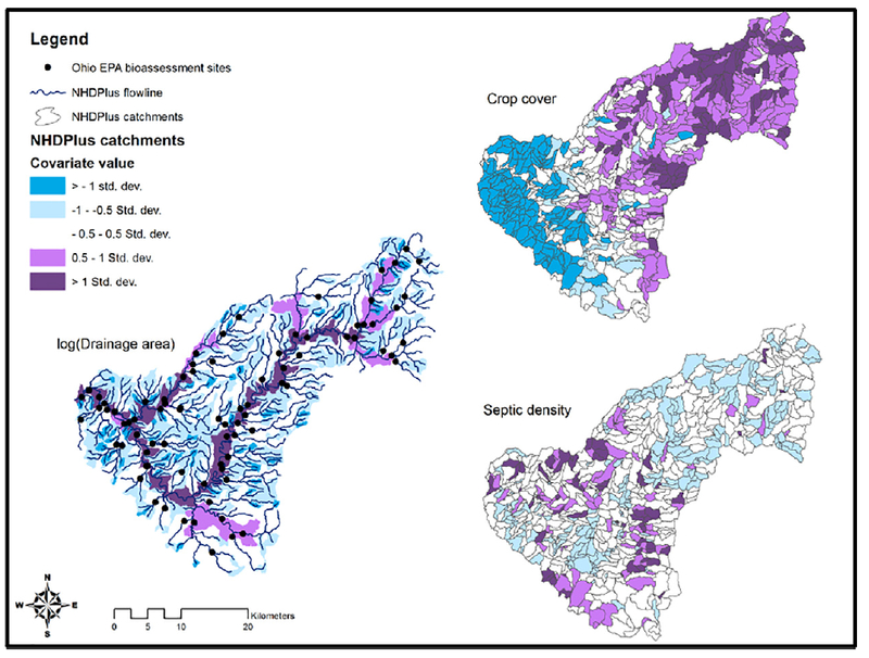
Maps of values for landscape-based covariates used as predictors in the case study application; locations of OEPA bioassessment sites (N=83) across the EFLMR watershed, where empirical data on nutrient chemistry and stream fish community composition were collected; and boundaries of NHDPlus catchments (for crop cover and septic density maps only) which served as the fundamental spatial data framework for the case study modeling effort. Individual catchments are colored according to standard deviations from the population mean values (i.e., mean across all catchments) for consistency and comparison with the standardization used on predictors in the joint model inputs.

Septic systems are also expected to represent an important component of nutrient loading (Scown et al., 2017).

Although demonstrating cause and effect has proven difficult, the circumstantial case for a causal link between nutrient enrichment and aquatic community health is strong (Smith et al., 2007; Meador and Carlisle, 2007; Miltner, 2010). Nutrient enrichment indirectly affects sensitive fishes and macroinvertebrates by its effect on dissolved oxygen (DO) concentrations via increased microbial respiration (Sabater et al., 2000; Griffith et al., 2009). Nutrient enrichment is often related to bioassessment indicators of aquatic community condition (Heiskary and Markus, 2003; Miltner, 2010). For example, nutrient enrichment has been linked to degraded fish community health in Ohio streams (Miltner, 2010). Similar studies in the region have also demonstrated empirical associations between nutrients and periphyton, periphyton and DO, and DO and macroinvertebrates and fish (Griffith et al., 2009).

2.2. Empirical and geographic data

Data on stream fishes and nutrients from the EFLMR were provided by the Ohio Environmental Protection Agency’s (OEPA) Statewide Biological and Water Quality Monitoring and Assessment Program, and included 83 bioassessment sites collected over the summer of 2012 (Fig. 1). Although the fish community data were originally recorded in abundance format, the abundances were converted to presence-absence format (i.e., 0/1) for use in the joint model (see Methods: Model description). Though other enrichment sources have been demonstrated to correlate with aquatic community conditions in the region (e.g., nitrogen; Griffith et al., 2009; Miltner, 2010); to simplify the presentation for the objective of this paper, we focused only on total phosphorus (TP). In a recent study of Ohio streams, Miltner (2010) examined the effects of TP on fishes using statewide bioassessment data, and suggested a seasonal average for TP at 0.1 mg/L as a feasible management target for improving fish community health and to aid future abatement and prevention of eutrophication in Ohio streams (<1300 km² in drainage area; Miltner, 2010). We used this management criterion to examine the effects of excess nutrients on potentially sensitive fishes and their distributions. Thus, TP concentration data (mg/L) for each bioassessment site were converted to binary format depending on whether values were below or above 0.1 mg/L.

Three measures derived from GIS database sources were included for use as predictors in the model: drainage area, crop cover, and septic tank counts. It is well-known that fish assemblages sort strongly along drainage area gradients; and it has been demonstrated that drainage area is an important predictor of nutrient concentrations in this watershed (Scown et al., 2017). Though other landscape-based predictors may have provided some explanatory power in our analysis (e.g., soil type; Scown et al., 2017), we chose these two predictors because they are the primary landscape-based sources of anthropogenic stress in the watershed for which data was readily available. Though urban land cover is also a dominant, it is strongly and negatively correlated with agricultural land use across the watershed (unpublished analysis), which renders any effects measured as a result of agriculture difficult to interpret. Nevertheless, we opted to use agricultural land cover because of the more obvious common link to both TP and fishes.

Landscape-based data were quantified at the stream segment scale (1:100,000) defined by the vector-based, segment-level catchments within the NHDPlus hydrologic spatial dataset (Version 2; McKay et al., 2012). The catchment boundaries demark the land area estimated to drain to each segment. This topology enables straightforward quanti-fication of landscape-based conditions according to hydrologic structure (e.g., land use type as a proportion of drainage area; Wang et al., 2011); and the NHDPlus dataset is often used for evaluating ecological responses to landscape conditions across broad regions (e.g., Esselman et al., 2013; Phelan et al., 2017). In our example, these segment-level catchments represented the fundamental spatial unit of observation to which the empirical bioassessment data were spatially referenced. The catchments also served as the fundamental spatial unit for prediction and spatial projection of the model. Thus, all 815 segment-level catchments within the EFLMR HUC9 were included as part of the overall modeling effort (Fig. 1).

Spatial data on crop cover and drainage area were downloaded from the recently published StreamCat database, which includes a comprehensive list of segment and watershed-scale metrics for use with the NHDPlus dataset within the conterminous United States (Hill et al., 2016). The drainage area measure reflected watershed area (km²) at the corresponding NHDPlus stream segment outlet (Hill et al., 2016). Drainage area was log-transformed (natural log) for model input in order to linearize the relationship with responses. Crop cover reflected the cumulative, upstream watershed area classified as row crop land use (%), based on the 2011 National Land Cover Dataset (NLCD; Homer et al., 2011) classification (Hill et al., 2016). Finally, a catchment-level septic tank metric was derived from a spatial dataset of septic tank coverages over the HUC9 compiled by (Karcher et al., 2012) and recently implemented in Scown et al. (2017). We used this dataset to estimate the area of each catchment in the HUC9 containing septic structures. The septic data were provided as a 10 m resolution raster grid, where each 10 m by 10 m grid cell was dummy coded according presence/absence of septic tanks (i.e., 1 or 0). Thus, we estimated a coverage metric (%) for each catchment as:

$$septic\%=\frac{\left({\displaystyle {\sum }_{i=1}^{n}V}\right)\times 1.0e^{-6}}{A}$$

where V holds the value of each raster grid cell (i.e., 1 or 0) in the focal catchment, n is the number of cells within the focal catchment, and A is the area of the focal catchment (km²). The product term in the numerator converts the summation of the 10 m by 10 m grid cells to an area (km²).

2.3. Model description

For modeling the joint distribution of receptors and stressors as a function of linear predictors, we used the multivariate probit (MVP) model as formulated by Chib and Greenberg (1998) and introduced to ecologists by Latimer et al. (2009), and more recently by Clark et al. (2014) and Pollock et al. (2014). The MVP is applicable to response data recorded in the binary format (e.g., 0/1, −1/1; presence-absence) and models the probability of occurrence as the probability density of a latent variable exceeding a threshold. The basic model takes the form:

$$\begin{gathered} P\left(Y_{nd}=1\right)=P(Z_{nd}>0),forn=1,\mathrm{...},N;d=1,\mathrm{...},D \\ {Z}_n~N_d({\beta }_{d0}+{\beta }_{dk}{X}_n,\Omega ) \\ {\beta }_{d0}~N\left({\mu }_{d0},{\sigma }_{d0}\right),ford=1,\mathrm{...},D; \\ {\beta }_{dk}~N({\mu }_{dk},{\sigma }_{dk}),ford=1,\mathrm{...},D;k=1,\mathrm{...},K \end{gathered}$$

Therefore, the response matrix Y of receptor(s) and/or stressor(s) occurrences has dimensions N sites by D receptor(s)/stressor(s), with elements Y_nd, representing the response of the d^threceptor/stressor in the n^th site. The response data is binary, such that if the d^threceptor/stressor in the n^th site is present, then Y_nd=1 and, if absent, Y_nd=0. The predictor variable matrix X has dimension n sites by k predictors. The mean vector of each multivariate normal distribution, Z_n, is the sum of the corresponding intercept parameter, β₀, and the inner product of the corresponding row vector of X_n and a D by K coefficient matrix, β_dk. Thus, the rows, Z_n, of the latent variable matrix each follow D-dimensional multivariate normal distributions, which are governed by a common correlation matrix Ω. This D by D correlation matrix governs the correlations among responses and conforms to a unit variance along the diagonal to satisfy the constraint of probit regression, such that the regression coefficients can be interpreted on the probit scale (Chib and Greenberg, 1998), where:

$$Probit(P(Y_n=1))={\beta }_0+{\beta }_1{X}_{n1}+{\beta }_2{X}_{n2}+{\beta }_3{X}_{n3}+\mathrm{...}+{\beta }_k{X}_{nk}$$

For this latent variable parameterization, interpreting the posterior distribution of Z is perhaps easiest to conceptualize by first envisioning a single, latent response vector, Z_n. In analogy to a standard, univariate probit regression, where the latent response is modeled as a continuous, unconditional normal random variate with mean ψ and variance fixed at 1. The continuous latent-scale variate is converted to the 0–1 probability scale via the standard normal cumulative distribution function, Φ(Z_n). Thus, probability of presence is higher for larger values of Z_n, lower at smaller values, and exactly 0.5 when Z_n=0. In the multivariate problem, however, multiple responses are modeled via a multivariate analog, ψ_d. The multivariate mean can then be governed by the linear predictor, β_d0+X_nβ_dk, and the covariance matrix, Ω_dd, is introduced with the diagonal variances fixed at 1. The off-diagonals of the covariance matrix represent pairwise correlations among the responses and govern the joint, but not the unconditional (i.e., marginal) probabilities of presence and absence. In other words, the off-diagonals determine the probability of co-occurrence, which increases or decreases with the magnitude of Ω_dd, but not the unconditional probability of occurrence for individual responses, which is governed by the linear predictor, β_d0+X_nβ_dk (Chib and Greenberg, 1998; Pollock et al., 2014). In the practical sense, the linear predictor governs variability in the responses due to the measured environmental processes, whereas the off-diagonals of Ω capture associations among responses due to remaining (i.e., residual) dependencies, including dependencies induced by unmeasured environmental correlates, as well as dependencies resulting from stressor-receptor, stressor-stressor, or receptor-receptor interactions or (sensu Clark et al., 2014; Pollock et al., 2014). We also note that, in the form of the model we have presented, not all responses need have the same predictors; as each β_dk is sampled from an independent prior. Thus, one could include different predictors for different receptors or stressors in the model.

To better understand the information contained in the joint posterior, Z, first consider the simplest two-dimensional form (i.e., D=2): the bivariate probit formulation describing the joint density of two responses: Z_n1 and Z_n2. The joint posterior probability, P(Z_n1,Z_n2), can then be envisioned as a bivariate normal density, such that the unconditional probability of presence of each response corresponds to the univariate normal density along either axis of the bivariate normal. Thus, the location of each density along the bivariate axes determines the unconditional probability of presence for the corresponding variate, Z_nd; whereas the shape (i.e., circle to ellipse-like) and orientation (i.e., positive or negative slope) of the bivariate density determines the joint probability of presence (i.e., co-occurrence; see Pollock et al., 2014 for a graphical presentation of this concept).

2.4. Case study model inputs

The response data, Y, comprised empirical data from 28 responses measured across 83 sites in the EFLMR watershed; with 27 of the responses corresponding to records of presence-absence for fishes and 1 response corresponding to records of TP exceeding the management threshold of 0.1 mg/L. Although 77 fish species were encountered and noted in the bioassessment data, in this example, we excluded species with extremely low (<20%) or high (>80%) prevalence in order to minimize the effect of low information response vectors on model fitting; which can arise, for example, in the form of semi- or complete separation (Albert and Anderson, 1984). Separation issues can arise when, for example, a particular species is present in all sites above a specific drainage area value in the data, and absent in all sites with smaller drainage areas. In our experience with this particular dataset, including a large number of low-information responses (i.e., those with very high or very low prevalence in the dataset) modeled via a common weakly informative prior induced difficulty for the sampling algorithm (i.e., sub-optimal fit diagnostics; unpublished analyses). We note that this problem is not specific to this modeling method, as responses with all or nearly all presences or absences are unlikely to yield much information using any method, particularly when N is small. However, the Bayesian method affords some means for obtaining estimates even for such low information, binary data. For example, well-thought-out weakly informative or informative priors are often useful for addressing such issues (e.g., semi- and perfect separation; Gelman et al., 2008); and, in theory, we could have chosen different types of priors (e.g., informative, weakly informative) for each parameter and response combination in order to sufficiently fit a model including all 77 responses. However, for this example, the primary goal was to facilitate understanding of the general modeling framework within the context of a practical co-occurrence problem. Therefore, to reduce the complexity of the case study analysis and code, and because such responses were expected to yield very little to inference, we elected to remove data on low-information responses from the model in order to facilitate a satisfactory fit using a single, weakly informative prior applied across all of the β-parameters (see Appendix B for further information on priors).

All predictor variables were standardized prior to input into the MVP model by subtracting the mean and dividing by 2 standard deviations (Gelman et al., 2008). In the context of regression modeling, this standardization places continuous predictor variables on the same scale as binary predictors, enables clearer interpretation of effects across predictors, and facilitates assignment and interpretation of default priors for regression (Gelman et al., 2008).

2.5. Model fitting and checking

All information regarding prior distributions used in our examples has been provided as a supplement to this article (Appendix B). All models were fit using the Hamiltonian Monte Carlo (HMC) modeling software Stan v2.11.1 (Stan Development Team, 2016b) and RStan (Stan Development Team, 2016a), the R v3.3.1 (R Core Team, 2016) interface to Stan. Although similar models have been implemented for other popular sampling algorithms (e.g., Gibbs sampling; Pollock et al., 2014), the simultaneous updating of all parameters via the No-U-Turn sampler for HMC in Stan was expected to result in faster convergence and more effective sampling (Hoffman and Gelman, 2014; Monnahan et al., 2016). For the case study model, we ran four chains in parallel for 1000 HMC iterations. We assessed convergence by visually inspecting the trace plots, examining effective sample sizes (i.e., $n_{eff}>\left(-n_{iterations}\right)\times 0.1$, and assessing the Gelman-Rubin potential scale reduction factor (i.e., R_hat<1.1; Gelman and Rubin, 1992; Brooks and Gelman, 1998).

Model fit was evaluated using a number of posterior predictive model checking (PPMC) approaches (Gelman et al., 1996; Gelman et al., 2014). As the basis of our PPMC process, we (1) generated draws from the posterior parameters; (2) used those draws to generate new predictions for replicate datasets; and (3) compared the observed data to the distributions of replicated data. Specifically, we (1) compared rates of prevalence for responses in the empirical data to the posterior predictive distribution of rates in replicate data; and (2) compared observations of presence-absence for all responses across all sites to the posterior predictive distribution of probability of presence in replicated data. Finally, for selected responses, we also (3) constructed posterior predictive distributions for probability of presence and probability of co-occurrence for 100 replicated observations in a counterfactual analysis of the model-inferred predictor effects (McElreath, 2016). This allowed us to evaluate how predictions were expected to change across the range of predictor inputs, one predictor at a time. We assessed the counterfactual trends against the empirical observations across the range of predictor inputs. All PPMC-related plots (Appendix A) and code (Appendix C) are provided as a supplement to this article.

2.6. Predictions

Bayesian models are generative, treating all unknown parameters as random variables, including new observations that could arise from the same model. For example, posterior predictions for unobserved sites, Y_new, are simply additional estimates conditional on the posterior density of the parameters fit to Y_data. Therefore, Y_new are also probability densities and reflect sampling and parameter uncertainty. For our model, we used Stan to calculate the marginal posterior predictive distributions for all responses on the latent scale, Z_pred, for all sampled and unsampled segment-level catchments in the EFLMR watershed. Within R, we converted the latent scale predictions to the probability scale, via:

$$\Phi \left(Z_{pred}\right)=Y_{pred}$$

The conversion (pnorm function of base package in R) resulted in estimates, including uncertainty, for the marginal probability of presence for each response in the dataset at every EFLMR catchment. We also used R to calculate co-occurrence probabilities, including uncertainty, for the response groupings of interest; utilizing the latent scale, unconditional probability predictions, Z_pred, and posterior distributions for Ω. Specifically, to estimate the co-occurrence of a single species and TP exceedances, we used the multivariate cumulative distribution function (pmvnorm function in mvtnorm package; Genz et al., 2016) to calculate:

$$P\left(y_{n1}=1,y_{n2}=1\right)={\Phi }_2\left(z_{n1},z_{n2},{\rho }_{1,2}\right)$$

where ρ indicates the off-diagonals of Ω corresponding to the posterior distribution for the residual correlation of the two responses. Full posterior and posterior predictive distributions for all estimates and calculations are provided as a supplement to this article (Appendix D). Likewise, R code used in calculating probabilities described above is included as a supplement (Appendix C).

To summarize the probabilistic predictions graphically, for each response of interest, we constructed caterpillar plots detailing the distribution quantiles for each catchment-level prediction in the EFLMR. To visualize the predictive results spatially, we summarized the posterior predictive distributions for each catchment in two ways: (1) as single values reflective of location (i.e., posterior median of p), and (2) as single values reflecting certainty in the estimated probability (e.g., probability p>0.5). The summarized values were linked to the GIS for visualization via the NHDPlus COMID identifier unique to each catchment in the spatial database. All spatial data and resulting figures were constructed and viewed using ArcGIS 10.3.1 (ESRI, 2016).

3. Results

From the posterior distributions for covariate parameters (β), we inferred varied support among the 28 responses for non-zero effects; and parameter uncertainties were often high relative to the Probit scale (Fig. 2). The drainage area parameter estimates (β_log(AREA)) suggested that the unconditional probability of presence for most responses increased with stream size (Fig. 2). Only orangethroat darter (Etheostoma spectabile), western blacknose dace (Rhinichthys atratulus), white sucker (Campostoma commersoni), and johnny darter were predicted, with relatively high certainty (i.e., 90% credible interval excluding zero), to be more prevalent among smaller streams. For some species, including yellow bullhead (Ameiurus natalis), silverjaw minnow (Ericymba buccata), striped shiner (Luxilus chrysocephalus), largemouth bass (Micropterus salmoides), and scarlet shiner (Lythrurus fasciolaris), the 90% credible interval included both positive and negative estimates, suggesting greater uncertainty in the direction of the true effect. Nevertheless, the narrow intervals suggested the effects of drainage area were likely relatively small, regardless of direction. Finally, for some species, including golden redhorse and smallmouth bass (Micropterus dolomieu), the estimated effect was very uncertain and large relative to the probit scale, suggesting partial or complete separation of the data for these species along the covariate (see Methods).

Fig. 2.

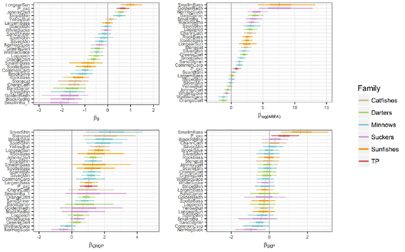
MVP model parameter summaries from the case study example (N=83 sites) illustrating modeled posteriors (horizontal bars) for all 27 species included in the model and the total phosphorus (TP) criterion. Panels include the intercept (β₀) of the linear predictor and parameters for the effects of the standardized predictors, including drainage area (β_log(AREA)), crop cover (β_CROP), and density of septic systems (β_SEP). Posterior distributions for the fishes are color-coded according to family, whereas posteriors for TP are color-coded in red. Short, vertical bars indicate posterior medians, whereas horizontal bars indicate 50% (thick bars) and 90% (thin bars) credible intervals. Effects were vertically ordered in each panel according to the posterior median. All predictors were first standardized by subtracting the mean and dividing by 2 standard deviations.

Posterior intervals for the crop cover coefficient (β_CROP) were also wide, indicating relatively high uncertainty in this parameter estimate, in general; though most responses were likely positively associated with this land use metric (Fig. 2). For other responses, the 90% credible interval included support for both positive and negative effects, indicating greater uncertainty regarding the direction of the effect. Only for northern hogsucker and western blacknose dace did the posterior suggest that the response direction was negative, though the credible intervals also included some support for zero or small positive effects.

Few of the septic cover posteriors (β_SEP) indicated clearly positive or negative associations with high certainty, though most posterior medians (i.e., expectations) were negative (Fig. 2). However, the posterior distribution of this parameter for smallmouth bass suggested, with relatively high certainty, that this species was more likely to be present in catchments with higher percentage [or density] of septic tanks. The magnitude of the effect was less certain, however, with the 90% credible interval ranging from relatively moderate values, on the Probit scale, to very high values. A positive association was also indicated between the septic coverage metric and TP exceedances. Finally, only northern hogsucker (Hypentelium nigricans) appeared to be negatively associated with this metric with relatively high certainty.

Estimates of residual correlation, which indicated the strength of dependencies among the responses after accounting for environmental effects, were relatively weak overall; though some estimates were precise enough to rule out zero correlation on the basis of the 90% credible interval (Fig. 3; see Appendix D for full posterior summaries).

Fig. 3.

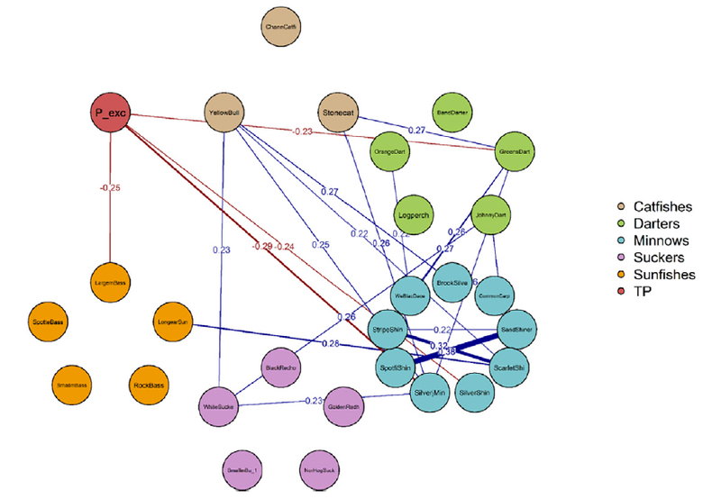
Network diagram depicting posterior medians of residual correlations (Ω) among the 28 model responses after accounting for the effects of environmental predictors. Only correlations where the 90% credible interval did not include zero are shown. Blue lines indicate positive correlation while red indicate negative correlation. The magnitude of correlation, summarized as the posterior mode, is indicated along line midpoints. TP response indicated by “P_exc”.

All negative correlations where the 90% credible interval did not include zero were correlations of fishes with TP exceedances. Aside from largemouth bass, all of those negative correlations were between TP and small-bodied, sensitive fishes, including greenside darter (Etheostoma blennioides), sand shiner (Notropis stramineus), silver shiner, and silverjaw minnow. Of those associations, the strongest negative correlation, based on the posterior median, was between silverjaw minnow and TP. However, due to uncertainty, we could not conclusively distinguish empirical differences in the strengths of those associations. Positive correlations where the 90% credible interval excluded zero, on the other hand, were all between fishes (Fig. 3). Of these, yellow bull-head had the most positive correlations to other species, including correlations with white sucker, striped shiner, scarlet shiner, and brook silverside (Labidesthes sicculus). The strongest correlations, in terms of the posterior median, were among the minnows, including between the sand shiner and spotfin shiner (Cyprinella spiloptera), and between the striped shiner and scarlet shiner.

To evaluate the implications of the model within a spatial context, we mapped predictions for silverjaw minnow, TP, and their co-occurrence; since inference from the posterior correlations suggested this to be the strongest negative association of practical interest (i.e., a negative interaction between the potential stressor and fish; Fig. 4).

Fig. 4.

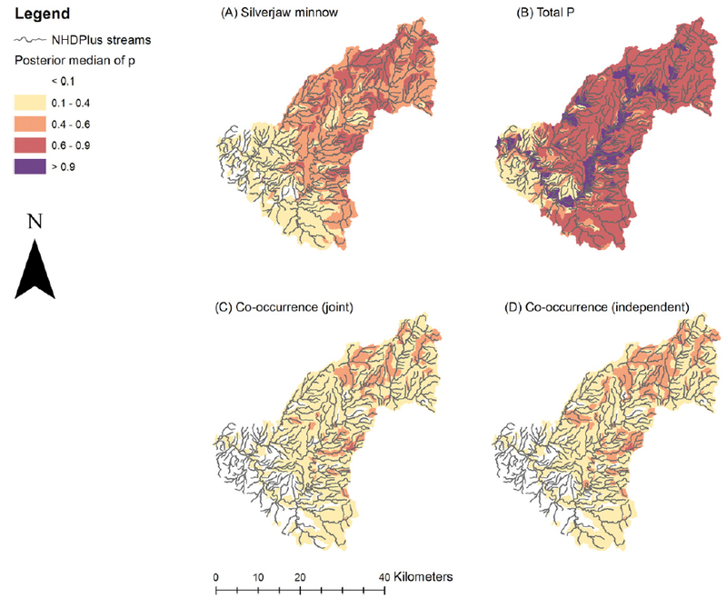
Maps illustrating the spatial distribution of predicted occurrence and co-occurrence of silverjaw minnow and TP exceedances, based on the median of the posterior predictive distributions generated from the case study model derived from empirical distribution data from N=83 sites. Map panels indicate (A) the marginal probability of presence for silverjaw minnow; (B) the marginal probability of TP exceedance; (C) the probability of co-occurrence of silverjaw minnow and TP exceedance based on the joint distribution; and (D) the probability of co-occurrence of silverjaw minnow and TP exceedance, when assuming the two responses are statistically independent (i.e., Ω=0).

The posterior medians of the unconditional probability of presence of silverjaw minnow were highest among tributaries in the middle and northeast portions of the watershed (Fig. 4A). However, TP exceedances were most common among mainstem EFLMR catchments (Fig. 4B). TP exceedances were also common in smaller tributaries, particularly in the crop-dominated areas in the northern three quarters of the watershed. In general, TP exceedances were relatively ubiquitous throughout the watershed, with the lowest probabilities predicted among the smaller tributaries of the southwest, where crop cover was of relatively low proportion.

Posterior medians for probability of co-occurrence of silverjaw minnow and TP exceedance were highest among the smaller tributaries of the northeastern half of the watershed where crop cover was highest (Fig. 4C), which follows from inference on the environmental predictors, since each of these responses responded similarly along crop cover gradient (Fig. 2). Nevertheless, the magnitudes of the posterior medians were generally moderate (i.e., 0.4<p<0.6), even for areas where predicted probabilities were highest.

To illustrate the effect of the negative empirical association among TP and silverjaw minnow captured by the joint model (i.e., Fig. 3) on the predictions, we constructed a separate map (Fig. 4D) of the posterior median of the probability of co-occurrence, which was calculated under the assumption that the responses were independent (i.e., as the product of the two unconditional response distributions, or where ρ=0; see Methods). Though differences between the two maps are subtle, due to the modest magnitude of the empirical dependence between the two responses (i.e., posterior median ρ= −0.29; Fig. 3), it can be seen that the joint estimate (Fig. 4C) generally projected lower co-occurrence probabilities, by comparison to the estimates assuming independence (Fig. 4D).

Finally, whereas the posterior median estimates summarize expectations, the posterior predictive distributions can also be summarized to facilitate evaluation of predictive uncertainty. For example, graphical summaries of the posterior predictive distributions for TP exceedance and silverjaw minnow suggested that uncertainty regarding the unconditional probability of presence for both responses was generally high (i.e., wide credible intervals; Fig. 5).

Fig. 5.

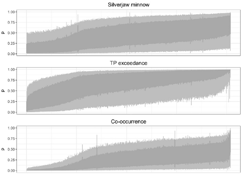
Graphical summaries of the posterior predictive distributions from the case study model, based on empirical distribution data from N=83 sites, for silverjaw minnow, TP exceedance, and their co-occurrence for each of the 815 catchments in the EFLMR HUC9. The panels show (top) the unconditional probability of presence of silver jaw minnow, (middle) the unconditional probability of TP exceedance, and (bottom) the joint probability of their co-occurrence. The graphed summaries depict the 50% (dark gray, vertical bars) and 90% (light gray, vertical bars) credible intervals for each catchment. The summaries were ordered, left to right, based on the value of the posterior median for each catchment.

The graphical summaries also suggested that, for silverjaw minnow, catchments where the posterior median probability was low were generally predicted with greater certainty (i.e., narrower credible intervals). Conversely, for TP exceedance, catchments where the posterior median probability was high were estimated with greater certainty (Fig. 5). Lastly, certainty regarding probability of co-occurrence was greater among catchments where the posterior median probability was low, compared to catchments where the posterior median probability was higher (Fig. 5).

Mapped summaries of the posterior predictive distributions of the probability of co-occurrence among catchments for these two responses provided a spatial context for visualizing this pattern in uncertainty (Fig. 6).

Fig. 6.

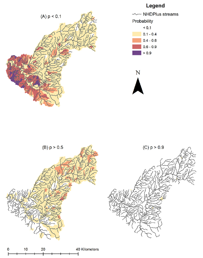
Maps illustrating spatial variability in predictive certainty following from the case study model based on empirical distribution data from N=83 sites. Map panels indicate spatial variability in (A) the posterior probability that co-occurrence probability, p, is very low, or less than 0.1; (B) that p is greater than 0.5, or more likely than not; and (C) that p is very high, or greater than 0.9.

Overall, the graphical summaries and maps suggested that identifying catchments where co-occurrence is unlikely (e.g., p<0.1), may generally be done with greater certainty compared to identifying catchments where co-occurrence is highly likely (Figs. 5 and 6). More practically, the maps suggest that we could rule out, with considerable certainty, many of the catchments in the southwest corner of the water-shed, where crop cover is relatively low, as being conducive to co occurrence. On the other hand, it would be difficult to pinpoint any particular catchment, with a high degree of certainty, as being very likely to have co-occurrences; though such events are likely relatively common throughout the watershed.

4. Discussion

The joint modeling approach is increasingly recognized as broadly applicable to a wide range of ecological research questions (Warton et al., 2015a; Clark et al., 2017; Ovaskainen et al., 2017). The goal of this study was to extend that utility to the problem of assessing co-occurrences between potential stressors and sensitive ecological receptors in the context of assessing ecological exposures. Our case study results highlighted the joint model’s ability to derive inference relevant to this problem from empirical distribution data. For example, phosphorus enrichment is considered a leading cause of impairment to rivers and streams in the United States (USEPA, 2007); and recent regional studies have outlined a causal path of empirical associations from phosphorus to periphyton, from periphyton to DO, and from DO to macroinvertebrates and fishes (Miltner, 2010; Griffith et al., 2009). Inference from our model suggested evidence of negative, albeit relatively weak, correlations between the distribution of TP criterion exceedances and the distributions of some fishes. Aside from largemouth bass, all of the fishes that were negatively correlated with the TP criterion exceedances are also considered pollution-sensitive in the region (Ohio EPA, 1987). Thus, inference from the model was generally consistent with the notion that sensitive fishes may be negatively, if indirectly (i.e., low DO concentrations; Smale and Rabeni, 1995), impacted by nutrient enrichment (Wang et al., 2007; Miltner, 2010).

In addition to accounting for potential stressor-receptor, receptor-receptor, or stressor-stressor interactions in the residual term, the joint model provides inference regarding environmental influences on co-occurrence. For example, the posterior distributions of the β-parameters for TP exceedance and silverjaw minnow suggested an environmentally-induced correlation between the two responses (sensu Pollock et al., 2014), because both responded in a similar manner to landscape-based predictors, namely drainage area and crop cover. That high TP concentrations are correlated with agricultural land cover is not particularly surprising. However, the mechanisms linking agricultural land cover to silverjaw minnow prevalence, as well as most of the fishes included in the model, is less clear. One explanation is that any effect of increasing agricultural land use, in this particular study, is likely indistinguishable from the effects of simultaneously declining urban cover. In fact, forest, urban, and agricultural land cover are all strongly correlated in the dataset as a result (unpublished analyses). Conclusions from other studies investigating the effects of urban land cover on stream fishes within agricultural regions suggest that the effects of urbanization may often outweigh those of agricultural development (Klauda et al., 1998; Wang et al., 2001). Thus, the positive effect of agricultural land cover on the prevalence of many fishes seen in our study may actually reflect some relative benefit associated with declining urbanization. Nevertheless, exploiting this empirical association ultimately reduced predictive uncertainty and, though not directly intuitive, provided information that could be used to refine future hypotheses and study objectives (e.g., broader sampling across land use types).

Separation of the environmental (i.e., linear predictor) and residual effects is an important property of the joint model that makes it uniquely appropriate for the co-occurrence problem. Specifically, the unconditional probabilities of occurrence of pairs of responses are used in conjunction with the quantified residual dependence to calculate an unbiased probability of co-occurrence (Pollock et al., 2014). Besides proper statistical accounting of system dependencies and uncertainty, however, another advantage of this model structure is that we can speculate independently about the effects of each component (i.e., environmental or residual) while ignoring the other. For example, the inferred, environmentally-induced correlation between TP exceedances and silverjaw minnow presence in our study suggests that co-occurrence would be more frequent in catchments where environmental conditions were favorable to both, were they not also directly and negatively correlated, as suggested by the residual term. In our presentation, we calculated and mapped co-occurrence probabilities for TP and silverjaw minnow based solely on this environmental component (i.e., co-occurrence probability calculated as the product of the unconditional probabilities of occurrence). From a practical perspective, mapping this calculation may be useful for examining where, for example, silverjaw minnow may have been reasonably likely to occur, were high TP not an issue (i.e., Fig. 4D).

In our example, we first applied the model as a tool to derive inference from a complex ecological system where environmental and biological dependencies were relatively unknown; and then let that inference drive subsequent decisions for evaluating specific ecological, predictive, and spatial implications. Ultimately, we presented figures and maps for evaluating the co-occurrence of TP exceedances and silverjaw minnow, because the model inferred that their negative interaction was potentially the strongest. We believed this approach to be reasonably representative of a practical scenario where, for example, managers aim to establish an empirical basis for distinguishing among regions of a watershed according to the probability of containing potentially detrimental combinations of receptors and stressors. Thus, our example emphasizes the utility of the approach in cases where the ecotoxicological dependencies are relatively unknown. Nevertheless, it would also be reasonable to apply this framework to problems where the associations among stressors and receptors are better understood, as a tool primarily for empirical validation or prediction. In fact, the multivariate response matrix can accommodate problems ranging from a single receptor and stressor to those involving multiple receptors and stressors. However, we emphasize that, where empirical data are available, a more inclusive response matrix could ultimately broaden inference and improve predictions. The joint formulation exploits all predictive associations, thus, including more responses may ultimately improve predictive accuracy and reduce uncertainty (Warton et al., 2015a; Clark et al., 2014). Likewise, a more inclusive response matrix of receptors and stressors could afford a more comprehensive perspective of ecological dependencies and risks, which could be informative for practical questions concerning scope and complexity, particularly in early assessment phases (e.g., USEPA, 1998).

Uncertainties associated with the regression parameters and predictions were relatively high overall in our case study, as may be expected given the relatively small sample size for a binary response type (i.e., N=83). Nevertheless, exploring the posterior predictive summaries graphically and spatially enabled us to refine our expectations regarding co-occurrence, on the basis of certainty, beyond what might be gleaned from looking only at point estimates from a more traditional approach (e.g., regression via maximum likelihood). Likewise, though maximum likelihood-based programs exist for this type of modeling (e.g., Yee, 2007), we believe the Bayesian approach generally offers greater flexibility, which may translate to broader utility in practice. For example, the Bayesian approach affords the use of prior information, which can be particularly useful in small data problems (Gelman et al., 2014). In our example, we employed weakly informative, regularizing priors (Gelman et al., 2008), which allowed us to include additional species in the model with relatively low or high prevalence in the empirical dataset. This would likely have been intractable using maximum likelihood approaches due to issues such as perfect or semi-separation (Gelman et al., 2008).

Whereas other recent studies have presented spatially-informed approaches to the co-occurrence problem in the context of ecological exposures, many appear to be semi-quantitative (e.g., Jackson et al., 2004; De Lange et al., 2010; Fox et al., 2016). Indeed, data complexities and study goals often necessitate such approaches, which are generally considered an improvement over qualitative approaches (Cox et al., 2005). Nevertheless, such approaches often only provide estimates of relative measures and lack an explicit framework for dealing with statistical dependencies and uncertainty (Cox, 2008; Fox et al., 2016). Alternatively, under a single statistical model, the joint modeling framework is capable of linking both receptors and stressors to potential landscape-based sources (e.g., crop cover, septic prevalence), while also quantifying potential associations under a single statistical model. Sampling from the joint distribution under the Bayesian framework also enables propagation of uncertainty throughout all posterior parameters, including parameters representing predictions for new observations; making probabilistic prediction and inference straightforward. For example, we have shown how posterior predictive distributions can be summarized and spatially projected for use in distinguishing areas of potential co-occurrence, where sensitive receptors may be at risk, on the basis of modeled expectations and predictive uncertainty. Therefore, where sufficient empirical and spatial data are available, we believe the joint modeling approach offers a quantitatively explicit and statistically transparent modeling alternative to semi-quantitative approaches for evaluating co-occurrences.

Limitations and extensions of the fundamental JSDM framework presented in this paper have been well documented in the applied ecological literature (Pollock et al., 2014; Clark et al., 2014; Clark et al., 2017; Ovaskainen et al., 2017). Nevertheless, we reiterate several important points to consider for practitioners interested in applying the framework to new or existing data. First, though careful study design and model building can improve inference and guide insight into causality, the joint model does not explicitly identify mechanisms, which can only be confirmed through rigorous experimentation. Residual associations estimated under the MVP likelihood, for example, could be a result of either true biological or toxicological interactions, or simply unmeasured effects of additional, known or unknown predictors or responses (Pollock et al., 2014). Thus, our case study results, which suggested biologically reasonable associations between TP and some fishes, should not be taken to imply a definitively causal relationship. Nevertheless, correlative results such as these can be useful for exploring and generating more targeted hypotheses, which could later be evaluated in experimental studies to establish causal links.

Second, our model assumed that residual associations were constant across the dataset and, thus, across the spatially projected predictions. This assumption could prove problematic when, for example, the true associations among stressors or sensitive species are context dependent, or modified by the presence of another measured or unmeasured stressor or species (e.g., Blaustein and Kiesecker, 2002). Generally, whereas model predictions and uncertainty are quantitatively exact in the Bayesian sense, inference ultimately remains conditional on any known or unknown biases inherent to the sampling strategy or chosen model parameterization. For example, projecting the case study model’s predictions to past or future conditions requires caution. This is because the bioassessment data reflected essentially a snapshot in time; thus, such projections are ultimately beyond the explicit scope of our model and data. Nevertheless, from a practical perspective, stream fish community structure in the region is generally thought to be stable over the index period from which they were sampled; and year-to-year variability is thought to be relatively low in comparison to site-to-site variability (Ohio EPA, 1987). Therefore, it may be reasonable to expect that predictions from the model are roughly applicable beyond the sample time frame. As is generally true with most modeling approaches, one should be both conscious and cautious of inferential extrapolations, which should be moderated transparently and according to practical knowledge of the system at study and a sound understanding of the model and data.

To conclude, the modeling framework presented in this paper generally parallels earlier JSDM implementations discussed in the applied ecological literature (e.g., Latimer et al., 2009; Clark et al., 2014; Pollock et al., 2014). To our knowledge, however, this paper is the first to present the framework in the context of evaluating ecological exposures. Our intention was to present the framework in a relatively basic form in order to promote a fundamental level of understanding of the key components of the approach. Yet, extending the model beyond this relatively basic parameterization is straightforward; as the joint modeling framework, in general, can accommodate a wide range of study designs (e.g., hierarchical, temporal, spatial), data types (e.g., dichotomous, continuous), and sampling strategies (e.g., estimating detection probability; Beissinger et al., 2016; Warton et al., 2016; Clark et al., 2017; Ovaskainen et al., 2017). In a comprehensive review of the joint modeling framework for use in community ecology research, for example, Ovaskainen et al. (2017) recently discussed applying model-based constraints to the species response matrix on the basis of phylogeny or ecological traits to further improve prediction and inference; an approach which could be similarly applied to stressor responses (e.g., based on physicochemical properties; Malaj et al., 2015). Moreover, with spatially or temporally structured data, relevant extensions have been discussed that could facilitate more explicit evaluations of species, receptor, and environmental associations across different spatial and/or temporal scales (Ovaskainen et al., 2017). Therefore, though we presented a useful and fundamental form of the JSDM, we stress that practitioners will likely benefit from consulting the rapidly developing JSDM literature, where computational efficiencies and extensions continue to both advance and generalize (e.g., Clark et al., 2017).

HIGHLIGHTS.

• Ecological risk managers assess potential for stressors and receptors to co-occur.

• A data-driven approach to modeling and mapping co-occurrences is presented.

• Model provides inference regarding ecotoxicological and environmental drivers.

• Mapped, probabilistic predictions afford a spatial construct for assessments.

• A study on stream fishes clarifies key model structures and practical utility.

References

- Albert A, Anderson JA, 1984. On the existence of maximum likelihood estimates in logistic models. Biometrika 71, 1–10. [Google Scholar]
- Barnthouse LW, Munns WR Jr.and Sorensen MT Population-level ecological risk assessment, 2008. Taylor & Francis; Boca Raton, FL, USA. [Google Scholar]
- Baselga A, Araujo MB, 2010. Do community models fail to project community variation effectively? J. Biogeogr 37, 1842–1850. [Google Scholar]
- Beissinger SR, Iknayan KJ, Guillera-Arroita G, Zipkin EF, Dorazio RM, et al. , 2016. Incorporation imperfect detection into joint models of communities: a response to Warton et al. Trends Ecol. Evol 31, 736–737. [DOI] [PubMed] [Google Scholar]
- Bhatt S, Gething P, Brady OJ, Messina JP, Farlow AW, Moyes CL, et al. , 2013. The global distribution and burden of dengue. Nature 496, 504–507. [DOI] [PMC free article] [PubMed] [Google Scholar]
- Blaustein AR, Kiesecker JM, 2002. Complexity in conservation: lessons from the global decline of amphibian populations. Ecol. Lett 5, 597–608. [Google Scholar]
- Brooks SP, Gelman A, 1998. General methods for monitoring convergence of iterative simulations. J. Comput. Graph. Stat 7, 434–455. [Google Scholar]
- Calabrese JM, Certain G, Kraan C, Dormann CF, 2014. Stacking species distribution models and adjusting bias by linking them to macroecological models. Glob. Ecol. Biogeogr 23, 99–112. [Google Scholar]
- Carola AS, Liess M, 2007. Mapping ecological risk of agricultural pesticide runoff. Sci. Total Environ 384, 264–279. [DOI] [PubMed] [Google Scholar]
- Chib S, Greenberg E, 1998. Analysis of multivariate probit models. Biometrika 85, 347–361. [Google Scholar]
- Clark JS, Gelfand AE, Woodall CW, Zhu K, 2014. More than the sum of the parts: forest climate response from joint species distribution models. Ecol. Appl 24, 990–999. [DOI] [PubMed] [Google Scholar]
- Clark JS, Nemergut D, Seyednasrollah B, Turner PT, Zhang S, 2017. Generalized joint attribute modeling for biodiversity analysis: median-zero, multivariate, multifarious data. Ecol. Monogr 87, 34–56. [Google Scholar]
- Core Team, R., 2016. R: A Language and Environment for Statistical Computing R Foundation for Statistical Computing, Vienna, Austria: https://www.R-project.org/. [Google Scholar]
- Cox LA, 2008. What’s wrong with risk matrices. Risk Anal. 28, 497–512. [DOI] [PubMed] [Google Scholar]
- Cox LA, Huber W, Babayev D, 2005. Some limitations of qualitative risk ranking systems. Risk Anal. 25, 651–662. [DOI] [PubMed] [Google Scholar]
- De Lange HJ, Sala S, Vighi M, Faber JH, 2010. Ecological vulnerability in risk assessment: a review and perpectives. Sci. Total Environ 408, 3871–3879. [DOI] [PubMed] [Google Scholar]
- Elith J, Leathwick JR, 2009. Species distribution models: ecological explanation and prediction across time and space. Annu. Rev. Ecol. Evol. Syst 40, 677–697. [Google Scholar]
- ESRI, 2016. ArcGIS Desktop: Release 10.3.1 Redlands. CA: Environmental Systems Research Institute. [Google Scholar]
- Esselman PC, Infante DM, Wang L, Cooper AR, Wieferich D, Tsang Y, et al. , 2013. Regional fish community indicators of landscape disturbance to catchments of the conterminous United States. Ecol. Indic 26, 163–173. [Google Scholar]
- Fischer KN, Suryan RM, Roby DD, Balogh GR, 2009. Post-breeding season distribution of black-footed and Laysan albatrosses satellite-tagged in Alaska: inter-specific differences in spatial overlap with North Pacific fisheries. Biol. Conserv 142, 751–760. [Google Scholar]
- Fox CH, O’Hara PD, Bertazzon S, Morgan K, Underwood FE, Paquet PC, 2016. A preliminary spatial assessment of risk: marine birds and chronic oil pollution on Canada’s Pacific coast. Sci. Total Environ 573, 799–809. [DOI] [PubMed] [Google Scholar]
- Franklin J, 2010. Mapping Species Distribution: Spatial Inference and Prediction Cambridge University Press, Cambridge, United Kingdom: 978–0–511–77006–7. [Google Scholar]
- Gelman A, Rubin DB, 1992. Inference from iterative simulation using multiple sequences. Stat. Sci 7, 457–511. [Google Scholar]
- Gelman A, Meng X, Stern H, 1996. Posterior predictive assessment of model fitness via realized discrepancies. Stat. Sin 6, 733–760. [Google Scholar]
- Gelman A, Jakulin A, Pittau MG, Su Y, 2008. A weakly informative default prior distribution for logistic and other regression models. Ann. Appl. Stat 2, 1360–1383. [Google Scholar]
- Gelman A, Carlin JB, Stern HS, Rubin DB, 2014. Bayesian data analysis Taylor & Francis, Boca Raton, FL, USA. [Google Scholar]
- Genz A, Bretz F, Miwa T, Mi X, Leisch F, Scheipl F, et al. , 2016. mvtnorm: multivariate normal and t distributions. R package version 1.0–5 http://CRAN.R-project.org/package=mvtnorm. [Google Scholar]
- Griffith MB, Daniel FB, Morrison MA, Troyer ME, Lazorchak JM, Shubauer-Berigan JP, 2009. Linking excess nutrients, light, and fine bedded sediments to impacts on faunal assemblages in headwater agricultural streams. J. Am. Water Resour. Assoc 45, 1475–1492. [Google Scholar]
- Guisan A, Rahbek C, 2011. SEASAM: a new framework integrating macroecological and species distribution models for predicting spatio-temporal patterns of species assemblages. J. Biogeogr 38, 1433–1444. [Google Scholar]
- Guisan A, Thuiller W, 2005. Predicting species distribution: offering more than simple habitat models. Ecol. Lett 8, 993–1009. [DOI] [PubMed] [Google Scholar]
- Guy TJ, Jennings SJ, Suryan RM, Melvin EF, Bellman MA, Ballance LT, et al. , 2013. Overlap of North Pacific albatrosses with the U.S. west coast groundfish and shrimp fisheries. Fish. Res 147, 222–234. [Google Scholar]
- Heiskary SA, Markus H, 2003. Establishing Relationships among in-Stream Nutrient Concentrations, Phytoplankton Abundance and Composition, Fish IBI, and Biochemical Oxygen Demand in Minnesota USA Rivers USEPA Region V, Minnesota Pollution Control Agency, USA, St. Paul, MN Final Report. [Google Scholar]
- Hill RA, Weber MH, Leibowitz SG, Olsen AR, Thornbrugh DJ, 2016. The stream-catchment (StreamCat) dataset: a database of watershed metrics for the conterminous United States. J. Am. Water Resour. Assoc 52, 120–128. [Google Scholar]
- Hoffman MD, Gelman A, 2014. The no-U-turn sampler: adaptively setting path lengths in Hamiltonian Monte Carlo. J. Mach. Learn. Res 15, 1593–1623. [Google Scholar]
- Homer CG, Dewitz JA, Yang L, Jin S, Danielson P, Xian G, et al. , 2011. Completion of the 2011 National Land Cover Database for the conterminous United States – representing a decade of land cover change information. Photogramm. Eng. Remote. Sens 81, 345–354. [Google Scholar]
- Jackson LE, Bird SL, Matheny RW, O’Neill RV, White D, Boesch KC, et al. , 2004. A regional approach to projecting land-use change and resulting ecological vulnerability. Environ. Monit. Assess 94, 231–248. [DOI] [PubMed] [Google Scholar]
- Karcher SC, Van Briesen J, Nietch CT, Heberling MT, Ramakrishnan B, 2012. Examining the Feasibility of Water Quality Trading in the East Fork Watershed Case Study. U.S. Environmental Protection Agency, Cincinnati, OH. [Google Scholar]
- Kery M, Royle JA, 2016. Applied Hierarchical Modeling in Ecology: Analysis of Distribution, Abundance and Species Richness in R and BUGS 1st Edition Academic Press & Elsevier, London, United Kingdom. [Google Scholar]
- Klauda R, Kazyak P, Stranko S, Southerland M, Roth N, Chaillou J, 1998. Maryland biological stream survey: a state agency program to assess the impact of anthropogenic stress on stream habitat quality and biota. Environ. Monit. Assess 51, 299–316. [Google Scholar]
- Lahr J, Kooistra L, 2010. Environmental risk mapping of pollutants: state of the art and communication aspects. Sci. Total Environ 408, 3899–3907. [DOI] [PubMed] [Google Scholar]
- Latimer AM, Banerjee S, Sang H, Mosher ES, Silander JA Jr., 2009. Hierarchical models facilitate spatial analysis of large data sets: a case study on invasive plant species in northeastern United States. Ecol. Lett 12, 144–154. [DOI] [PubMed] [Google Scholar]
- Loos M, Ragas AMJ, Plasmeijer R, Schipper AM, Hendriks AJ, 2010. Eco-SpaCE: an object-oriented, spatially explicit model to assess the risk of multiple environmental stressors on terrestrial vertebrate populations. Sci. Total Environ 408, 3908–3917. [DOI] [PubMed] [Google Scholar]
- Malaj E, Guenard G, Schafer RB, von der Ohe PC, 2015. Evolutionary patterns and physicochemical properties explain macroinvertebrate sensitivity to heavy metals. Ecol.Appl 26, 1249–1259. [DOI] [PubMed] [Google Scholar]
- McElreath R, 2016. Statistical Rethinking: A Bayesian Course with Examples in R and Stan Taylor and Francis, Boca Raton, FL. [Google Scholar]
- McKay L, Bondelid T, Dewald T, Johnston J, Moore R, Reah A, 2012. NHDPlus Version 2: User Guide. ftp://ftp.horizon-systems.com/NHDPlus/NHDPlusV21/Documentation/NHDPlus-V2_User_Guide.pdf. [Google Scholar]
- Meador MR, Carlisle DM, 2007. Quantifying tolerance indicator values for common stream fish species of the United States. Ecol. Indic 7, 329–338. [Google Scholar]
- Miltner RJ, 2010. A method and rationale for deriving nutrient criteria for small rivers and streams in Ohio. Environ. Manag 45, 842–855. [DOI] [PubMed] [Google Scholar]
- Monnahan CC, Thorson JT, Branch TA, 2016. Faster estimation of Bayesian models in ecology using Hamiltonian Monte Carlo. Methods Ecol. Evol 8, 339–348. [Google Scholar]
- Ohio Environmental Protection Agency, 1987. User’s manual for biological field assessment of Ohio surface waters Vol. II Division of Water Quality Monitoring and Assessment, Surface Water Section, Columbus, OH. [Google Scholar]
- Ovaskainen O, Tikhonov G, Nordberg A, Blanchet FG, Duan L, et al. , 2017. How to make more out of community data? A conceptual framework and its implementation as models and software. Ecol. Lett 10.1111/ele.12757. [DOI] [PubMed] [Google Scholar]
- Phelan J, Cuffney T, Patterson L, Eddy M, Dykes R, Pearsall S, et al. , 2017. Fish and invertebrate flow-biology relationships support the determination of ecological flows for North Carolina. J. Am. Water Resour. Assoc 53, 42–45. [Google Scholar]
- Pistocchi A, Groenwold J, Lahr J, Loos M, Mujica M, Ragas AMJ, Rallo R, Sala S, Schlink U, Strebel K, Vighi M, Viscaino P, 2011. Mapping cumulative environmental risks: examples from the EU NoMiracle project. Environ. Model. Assess 16, 119–133. [Google Scholar]
- Pollock LJ, Tingley R, Morris WK, Golding N, O’Hara RO, Parris KM, et al. , 2014. Understanding co-occurrence by modeling species simultaneously with a joint species distribution model (JSDM). Methods Ecol. Evol 5, 397–406. [Google Scholar]
- Sabater S, Armengol J, Comas E, Sabater F, Urrizalqui I, Urrutia I, 2000. Algal biomass in a disturbed Atlantic river: water quality relationships and environmental implications. Sci. Total Environ 263, 185–195. [DOI] [PubMed] [Google Scholar]
- Scown MW, McManus MG, Carson JH Jr., Nietch CT, 2017. Improving Predictive Models of In-Stream Phosphorus Concentration Based on Nationally-Available Spatial Data Coverages. JAWRA Journal of the American Water Resources Association. 53 (4): 944–960. 10.1111/1752-1688.12543. [DOI] [PMC free article] [PubMed] [Google Scholar]
- Smale MA, Rabeni CF, 1995. Influences of hypoxia and hypothermia on fish species composition in headwater streams. Trans. Am. Fish. Soc 124, 711–725. [Google Scholar]
- Smith AJ, Bode RW, Kleppel GS, 2007. A nutrient biotic index (NBI) for use with benthic macroinvertebrate communities. Ecol. Indic 7, 371–386. [Google Scholar]
- Stan Development Team, 2016a. Rstan: the R interface to Stan. http://mc-stan.org/, Version 2.10.1. [Google Scholar]
- Stan Development Team, 2016b. Stan modeling language users guide and reference manual. http://mc-stan.org/, version 2.11.0. [Google Scholar]
- USEPA, 2007. National Water Quality Inventory: Report to Congress, 2002 Reporting Cycle EPA 841-R-07–001. U. S. EPA, Washington, D. C. [Google Scholar]
- USEPA, 2010. Causal Analysis/Diagnosis Decision Information System (CADDIS) Office of Research and Development, Washington, D.C. https://www.epa.gov/caddis. [Google Scholar]
- USEPA (U.S. Environmental Protection Agency), 1998. Guidelines for Ecological Risk Assessment, Final EPA 630-R-95–0. U. S. EPA, Washington, D. C. [Google Scholar]
- USGS (U.S. Geological Survey), 2001. National Hydrography Dataset (NHD) Reston, Virginia: https://nhd.usgs.gov/, Accessed date: February 2017. [Google Scholar]
- Wang L, Lyons J, Kanehl P, 2001. Impacts of urbanization on stream habitat and fish across multiple spatial scales. Environ. Manag 28, 255–266. [DOI] [PubMed] [Google Scholar]
- Wang L, Robertson DM, Garrison PJ, 2007. Linkages between nutrients and assemblages of macroinvertebrates and fish in wadeable streams: implication to nutrient criteria development. Environ. Manag 39, 194–212. [DOI] [PubMed] [Google Scholar]
- Wang LZ, Brenden T, Seelbach P, Cooper A, Allan D, Clark R, et al. , 2011. A hierarchical spatial framework and database for the national river fish habitat condition assessment. Fisheries 36, 436–449. [Google Scholar]
- Warton DI, Blanchet FG, O’Hara RB, Ovaskainen O, Taskinen S, et al. , 2015a. So many variables: joint modeling in community ecology. Trends Ecol. Evol 30, 766–779. [DOI] [PubMed] [Google Scholar]
- Warton DI, Foster SD, De’ath G, Stoklosa J, Dunstan PK, 2015b. Model-based thinking for community ecology. Plant Ecol. 216, 669–682. [Google Scholar]
- Warton DI, Blanchet FG, O’Hara R, Ovaskainen O, Taskinen S, Walker SC, et al. , 2016. Extending joint models in community ecology: a response to Beissinger et al. Trends Ecol. Evol 31, 737–738. [DOI] [PubMed] [Google Scholar]
- Yee TW, 2007. bprobit: bivariate probit regression for dichotomous dependent variables In: Choirat C, Gandrud C, Honaker J, Imai K, King G, Lau O (Eds.), Zelig: everyone’s statistical software http://zeligproject.org/. [Google Scholar]
- Zydelis R, Lewison RL, Schaffer SA, Moore JE, Boustany AM, Roberts JJ, et al. , 2011. Dynamic habitat models: using telemetry data to project fisheries bycatch. Proc. R. Soc. B 278, 3191–3200. [DOI] [PMC free article] [PubMed] [Google Scholar]
Associated Data
This section collects any data citations, data availability statements, or supplementary materials included in this article.