Genome-wide association study for feed efficiency traits using SNP and haplotype models

Abstract

Feed costs comprise the majority of variable expenses in beef cattle systems making feed efficiency an important economic consideration within the beef industry. Due to the expense of recording individual feed-intake phenotypes, a genomic-enabled approach could be advantageous toward improving this economically relevant trait complex. A genome-wide association study (GWAS) was performed using 748 crossbred steers and heifers representing seven sire breeds with phenotypes for ADG and ADFI. Animals were genotyped with the BovineSNP50v2 BeadChip containing approximately 54,000 SNP. Both traits were analyzed using univariate SNP-based (BayesC) and haplotype-based (BayesIM) models and jointly using BayesIM to perform a bivariate GWAS. For BayesIM, a hidden Markov model (HMM) of haplotype segments of variable length was built where haplotypes were mapped to clusters based on local similarity. The estimated HMM was then used to assign haplotype cluster genotypes, instead of SNP genotypes, as latent covariates in a Bayesian mixture model. The number of haplotype clusters at each location was assumed to be either 8 (BayesIM8) or 16 (BayesIM16). A total of three univariate analyses for each trait and two bivariate analyses were performed. Posterior SD (PSD) for ADG were 0.28 (0.08), 0.37 (0.11), 0.37 (0.11), 0.35 (0.11), and 0.35 (0.12) for BayesC, BayesIM8, BayesIM16, BayesIM8 bivariate, and BayesIM16 bivariate, respectively. ADFI PSD were 0.30 (0.07), 0.44 (0.13), 0.42 (0.12), 0.38 (0.10), and 0.38 (0.10) for the same models. The top 1% of 1-Mb windows that explained the largest fraction of genetic variation in common between univariate SNP and haplotype models ranged from 24% to 40% and from 20% to 32% for ADG and ADFI, respectively. Spearmen rank correlations between molecular breeding values from SNP and haplotype-based models in the training data were similar for both traits (>0.96) suggesting that either model would lead to similar rankings of animals, although resolution of potential QTL appeared to be greater for BayesIM.

INTRODUCTION

The majority of variable expenses in beef cattle systems are due to feed costs making feed efficiency an important economic consideration (Koch et al., 1963; Dickerson et al., 1974). It is estimated that a 10% increase in daily gain would lead to an 18% advantage in profit, but a 10% increase in feed efficiency would increase profit by 43% (Fox et al., 2001). Aside from the economic considerations, improved feed efficiency also has an environmental impact as more efficient cattle have fewer days to finish and produce less methane throughout their lifetime (Freetly and Brown-Brandl, 2013). Moderate-to-high heritability estimates for feed efficiency traits (Arthur et al., 2001a, 2001b; Nkrumah et al., 2007) suggest feed efficiency would respond favorably to selection. Still, individual feed intake is difficult to obtain and expensive to measure. Therefore, a genomics approach seems warranted. Although genome-wide association studies (GWAS) have identified several QTL associated with feed efficiency traits (Snelling et al., 2011; Saatchi et al., 2014), none have compared a SNP-based approach with a haplotype-based approach. The objective of this study was to identify genomic regions associated with ADG and ADFI in an admixed population of beef cattle using univariate SNP and univariate and bivariate haplotype models.

MATERIALS AND METHODS

Description of Population

The experimental protocol at USMARC was approved by the USMARC IAACUC and followed FASS guidelines (FASS, 1999). Feedlot ADG and ADFI (on a DM basis) were recorded from crossbred steers and heifers (n = 777) at the U.S. Meat Animal Research Center (USMARC) in Clay Center, Nebraska, and the University of Missouri (MU) in Columbia, Missouri. Commercial dams were mated to seven purebred sire breeds including Angus, Red Angus, Charolais, Simmental, Hereford, Gelbvieh, and Limousin, and one commercial sire group comprised of ½ Angus, ¼ Simmental, and ¼ South Devon. The number of offspring by breed of sire is presented in Table 1.

Table 1.

Number of calves by sire breed

Sire breeda	No. Progeny
AN	204
AR	67
CH	64
COM	54
GV	148
HH	23
LM	73
SM	115

^aAN = Angus, AR = Red Angus, CH = Charolais, COM = Commercial, GV = Gelbvieh, HH = Hereford, LM = Limousin, SM = Simmental.

Animals used in the current study were the product of three matings across 2 yr and two locations. The first calf crop (n = 213) was born in May 2012 at a commercial ranch near Ashby, Nebraska. Calves were weaned in August of the same year and placed in a dry lot for backgrounding before entering individual feed-intake facilities. These steer calves were placed in GrowSafe facilities at MU with the 70-d feeding period beginning on March 20, 2013 and ending on May 30, 2013. Weights were recorded for two consecutive days at the start and end of the feeding period. Initial and final weights were determined as the mean of the two consecutive weights. While in the individual feeding facilities, the ration consisted of 8.9% corn silage, 52.1% whole corn, 26.4% DDGS, and 12.6% premix on a DM basis.

The second calf crop (n = 309) was born in August of 2012 at USMARC and weaned in January of 2013 into a feedlot. They were fed a backgrounding diet and entered Calan Gate feeding facilities at USMARC on July 9, 2013, and were removed on October 1, 2013, for a total of 83 days in the facility. Initial and final weights were estimated from the regression of BW on time across the entire feeding period. The on-test finishing ration consisted of 8% ground alfalfa, 67.75% rolled corn, 20% wet distillers grains with soluables, and 4.25% supplement containing rumensin at 700 g/ton on a DM basis. Steers were implanted with Revalor XS, and heifers were implanted with Revalor IH. Forty steers were used in a metabolism study prior to the feeding period, and therefore were treated as a separate contemporary group.

The final group of calves (n = 255) were born between April and May of 2013 at USMARC and weaned into the feedlot in September. They entered Calan Gate feeding facilities on February 11, 2014, and were removed from the facilities on May 6, 2014, for an 84-d feeding period. Initial and final weights were estimated from the regression of BW on time across the entire feeding period. The finishing ration and implant regimen were consistent with the 2012-born USMARC cattle.

Animals were genotyped with Illumina BovineSNP50v2 Beadchip (Illumina, San Diego, CA) that contained approximately 54,000 SNP.

Data Editing

Animals with unidentified sires or sire breeds (n = 6), those with missing birth dates (n = 19), missing genotypic data (n = 1) or late castrated steers (n = 3) were removed from the analysis. A total of 748 animals remained after data editing. Phenotypic means (SD) for ADG and ADFI after correcting for breed of sire, contemporary group (concatenation of location, year, and sex), and initial weight when entering the feeding facilities are presented in Table 2.

Table 2.

Number of observations (N) and mean (SD) for ADG and ADFI^a

Trait	N	Mean
ADG, kg/d	748	1.81 (0.22)
ADFI, kg/d	748	10.00 (1.13)

^aADG and ADFI adjusted for contemporary group (concatenation of year, location, and sex), breed of sire, and initial weight at the start of the feeding period.

Quality scores (GenCall) for each genotype were assigned through Illumina data analysis software. Missing genotypes or genotypes with GenCall scores less than 0.20 were replaced with the mean genotype score at that marker calculated within subgroups based on location and birth year. No preanalysis filtering was performed based on minor allele frequency. Unmapped and sex chromosome SNP were removed leaving 52,890 SNP for analysis.

Statistical Analyses

Both traits were analyzed independently through SNP (BayesC; Habier et al., 2011) and haplotype (BayesIM; Kachman, 2016) models and together using BayesIM to perform a bivariate GWAS. Contemporary group and breed of sire, with the composite sire group treated as its own breed, were fitted as a classification effects with initial weight, calculated as the average of the two consecutive weights at the start of the feeding period, fitted as a fixed covariate. BayesC was implemented via GenSel (version 0.9.2.045; Fernando and Garrick, 2009). The proportion of SNP assumed to have a null effect on the trait, π, was assumed to be 0.99 which corresponded to fitting approximately 500 markers in each Markov chain Monte Carlo (MCMC) iteration. A chain length of 41,000 iterations was run with the first 1,000 discarded as burn-in. Prior variance component estimates were selected by starting with low and high a priori heritability estimates until the posterior heritability estimates were trending up and down, respectively, and a value in the middle was chosen as the final a priori heritability estimate used to determine prior variance component estimates. The genome was separated into 1-Mb nonoverlapping windows (n = 2,536) with the additive genetic variance calculated within each window.

Haplotype association analyses were performed using a Bayesian mixture model fitting haplotype effects as covariates (BayesIM; Wilson-Wells and Kachman, 2016). A major limitation of current GWAS models is that they rely on information at the individual SNP locations. This is problematic because QTL are unlikely to be at the SNP location and it ignores information that could be garnered from using neighboring SNP loci. In brief, the haplotype-based model (BayesIM) partitions the genome into variable length segments. Haplotypes are clustered together based on similarity, and clusters are defined based on the frequency of the A allele at each locus. BayesIM models the haplotypes using a hidden Markov model where the hidden states are the unobserved haplotype cluster genotype, the transition probabilities are a function of the map distance between adjacent loci, and the emission probabilities are the frequency of the A allele at each locus. The number of haplotype clusters is considered fixed. Emission and transition probabilities for the hidden Markov model are estimated using maximum likelihood. Haplotype cluster segments are sampled using a Metropolis-Hastings algorithm. The sampled cluster genotype, instead of SNP genotype, are then used as covariates in the model. BayesIM is similar to well-known Bayesian mixture models used for GWAS such as BayesC (Habier et al., 2011) in that the probability of a nonzero haplotype effect at a given locus is given by 1-π where π is the probability that a haplotype (BayesIM) or SNP (BayesC) does not have an effect on the trait of interest. The same prior distributions for the fixed effects (flat), random effects (multivariate normal), and variances (inverse scaled chi-square) were assumed for both BayesIM and BayesC. Uniquely, BayesIM does not require that missing SNP be imputed, although in the present study we elected to do so to allow commonality of SNP genotypes between haplotype- and SNP-based models. The number of haplotype clusters at each location was assumed a priori to be either 8 (BayesIM8) or 16 (BayesIM16). A pooled-within sire breed genetic variance was calculated. To keep approximately equal number of covariates in the SNP and haplotype model, π was assumed to be 0.98 for both the univariate and bivariate haplotype analyses. The average haplotype length was estimated, and QTL were assumed to be evenly spaced every 100 kb. A total MCMC chain length of 100,000 iterations was used with the first 10,000 iterations discarded as burn-in. A prior heritability estimate was again selected by starting with low and high a priori heritability estimates until the posterior heritability estimates were trending up and down, respectively. A middle value was then chosen as the final a priori heritability estimate. Overlapping 1-Mb QTL regions (n = 25,200) were built in a stair-step fashion by offsetting the region starting position by 100 kb. From these QTL regions, 1-Mb nonoverlapping windows (n =2 ,536) were extracted for a direct comparison to the SNP-based model.

Calculation of Genetic and Residual Correlations

Bivariate haplotype analyses estimate the genetic and residual (co)variances for both traits in the model at each iteration. Given the additive genetic merit of the jth animal from j = 1,…, 748 is:

$$A_j={\displaystyle {\sum }_{i=1}^{25,200}{H}_i{G}_{ij}}$$

where H_i is the effect of the ith haplotype from i = 1,…, 25,200 and G_ij is the unobserved haplotype genotype of the ith haplotype for the jth animal, the additive genetic covariance between ADG and ADFI is derived as:

$${\sigma }_{A_{ADG,ADFI}}=\frac{{\displaystyle {\sum }_{j=1}^{748}\left(A_{AD{G}_j}-\stackrel{-}{A_{ADG}}\right)\left(A_{ADF{I}_j}-\stackrel{-}{A_{ADFI}}\right)}}{748}$$

where $A_{AD{G}_j}$ is the additive genetic merit of each animal from j = 1,…, 748 for ADG, $A_{ADG}$ is the mean additive genetic merit for ADG, $A_{ADF{I}_j}$ is the additive genetic merit of each animal from j = 1,…, 748 for ADFI, and $A_{ADF{I}_j}$ is the mean additive genetic merit for ADFI.

The genetic correlation was calculated as:

$$r_{A_{ADG, ADFI}}=\frac{{\sigma }_{A_{ADG, ADFI}}}{{\sigma }_{A_{ADG}}x{\sigma }_{A_{ADFI}} }$$

where ${\sigma }_{A_{ADG, ADFI}}$ is the additive genetic covariance between ADG and ADFI, ${\sigma }_{A_{ADG}}$ is the additive genetic SD of ADG, and ${\sigma }_{A_{ADFI} }$ is the additive genetic SD of ADFI.

The residual correlation was calculated as:

$$r_{E_{ADG, ADFI}}=\frac{{\sigma }_{E_{ADG, ADFI}}}{{\sigma }_{E_{ADG}}x{\sigma }_{E_{ADFI}} }$$

where ${\sigma }_{E_{ADG, ADFI}}$ is the residual covariance between ADG and ADFI, ${\sigma }_{E_{ADG}}$ is the residual SD of ADG, and ${\sigma }_{ADFI}$ is the residual SD of ADFI.

Calculation of Rank Correlations

A molecular breeding value (MBV) for each animal was estimated as the total genetic value of that individual based on the summation of the product of the marker effect and animal’s genotype across all loci. Pearson rank correlations were calculated based on MBV within trait for ADG and ADFI between all possible univariate analyses.

Gene Ontology

Top windows of interest were extended by 0.5 Mb in each direction to determine candidate genes associated with feed efficiency traits using the Bos taurus build UMD_3.1 assembly (Zimin et al., 2009). The BioMart data mining tool available through Ensembl (Ensembl Genes 84) was used to determine gene ontology terms of candidate genes.

RESULTS AND DISCUSSION

Posterior Mean Genomic Heritability Estimates

The posterior means of genomic heritability, additive genetic, and residual variances for ADG and ADFI are presented in Table 3. Posterior mean genomic heritability estimates for ADG ranged from 0.28 to 0.37 for the three univariate and two bivariate analyses with the SNP model producing the lowest estimate and the haplotype analyses being similar despite the number of haplotype clusters assumed. A similar trend was observed with ADFI as posterior mean genomic heritability estimates ranged from 0.30 to 0.44 with the SNP model again producing the lowest estimate.

Table 3.

Genomic heritability (h²), additive genetic variance (V_A), and residual variance (V_E) for ADG and ADFI^a

Trait	BayesC			BayesIM8b			BayesIM16c			BayesIM8 bivariateb			BayesIM16 bivariatec
	h2	VA	VE	h2	VA	VE	h2	VA	VE	h2	VA	VE	h2	VA	VE
ADG, kg/d	0.28 (0.08)	0.02 (0.01)	0.05 (0.01)	0.37 (0.11)	0.02 (0.01)	0.04 (0.01)	0.37 (0.11)	0.02 (0.01)	0.04 (0.01)	0.35 (0.11)	0.02 (0.01)	0.04 (0.01)	0.35 (0.12)	0.02 (0.01)	0.04 (0.01)
DMI, kg/d	0.30 (0.07)	0.28 (0.07)	0.67 (0.07)	0.44 (0.13)	0.40 (0.12)	0.51 (0.12)	0.42 (0.12)	0.39 (0.11)	0.53 (0.11)	0.38 (0.10)	0.36 (0.12)	0.59 (0.09)	0.38 (0.10)	0.36 (0.12)	0.59 (0.09)

^aEstimates are posterior means. Posterior SDs in parentheses.

^bBayesIM8 = BayesIM 8 clusters.

^cBayesIM16 = BayesIM 16 clusters.

Saatchi et al. (2014) reported genomic heritability estimates of 0.30 for ADG and 0.35 for ADFI from a BayesB model from an admixed population while Abo-Ismail et al. (2014) reported slightly higher estimates of 0.35 and 0.42 for ADG and ADFI, respectively. Pedigree-based estimates of heritability range from 0.23 to 0.41 for ADG and 0.27 to 0.54 for ADFI (Arthur et al., 2001a; Arthur et al., 2001b; Schenkel et al., 2004; Robinson and Oddy, 2004; Nkrumah et al., 2007). These results are in agreement with the findings of the current study. Differences between the haplotype- and SNP-based models may be due to the breed admixture of the population as BayesIM has the potential to be more sensitive to breed admixture with the HMM possibly building haplotype clusters that are breed specific.

Genetic and Residual Correlations From Bivariate Analyses

The posterior mean genetic correlations between ADG and ADFI were 0.59 (0.11) and 0.59 (0.10) for BayesIM8 bivariate and BayesIM16 bivariate, respectively. Previous estimates of genetic correlations between ADG and ADFI range from 0.50 to 0.87 (Arthur et al., 2001a; Schenkel et al., 2004; Nkrumah et al., 2007).

The posterior mean residual correlations between ADG and ADFI were 0.55 (0.06) and 0.55 (0.06) from BayesIM8 bivariate and BayesIM16 bivariate, respectively. Robinson and Oddy (2004) reported a higher residual correlation of 0.68 between feed intake and weight gain.

Rank Correlations of Molecular Breeding Values

Animals ranked similarly across SNP- and haplotype-based models for ADG with correlations >0.97. Rank correlations were similar for ADFI (>0.96). High rank correlation estimates between SNP and haplotype models indicated that both models would lead to similar animals being selected based on MBV.

Comparison of Genomic Regions Across Univariate SNP and Haplotype Models

The chromosomes and positions of top 1% of 1-Mb windows (n = 25) based on the percentage of genetic variance explained from univariate analyses are detailed in Table 4. The top 1% of 1-Mb windows (n = 25) from the bivariate analyses were determined by the top joint model frequency when both traits have a nonzero effect (Table 5). Commonality between top genomic regions across univariate SNP and haplotype models was described as the proportion of top 1% 1-Mb windows in common (Table 6).

Table 4.

Chromosome and position of the top 1% 1-Mb windows for ADG and ADFI from each univariate analysis^a

Chromosome	ADG			ADFI
	BayesC	BayesIM8b	BayesIM16c	BayesC	BayesIM8b	BayesIM16c
1			150–151	4–5, 150–151, 151–152	151–152, 155–156, 157–158	155–156, 157–158
2				14–15, 68–69		65–66
3	119–120	119–120	96–97	98–99	79–80	61–62
4	5–6	100–101	36–37
5						73–74
6	38–39		76–77	14–15	4–5, 14–15, 15–16, 16–17, 24–25	14–15, 16–17, 17–18
7		57–58, 67–68	64–65	102–103	26–27	14–15
8	1–2, 72–73	1–2, 6–7, 72–73	72–73, 92–93	82–83		107–108
9				101–102		20–21, 64–65
10	27–28, 45–46, 68–69, 101–102	101–102		20–21	41–42, 53–54
11	7–8	4–5	4–5		65–66
13	75–76, 81–82, 83–84	83–84	83–84	79–80, 82–83		25–26
14	13–14, 24–25	13–14, 24–25	23–24, 24–25, 26–27	9–10
15	81–82	26–27		20–21, 44–45, 82–83	44–45, 64–65, 71–72	44–45, 45–46, 64–65, 67–68, 82–83
16			24–25		21–22
17			65–66, 67–68		9–10
18	63–64	45–46	65–66
19	25–26	21–22	21–22	17–18, 30–31
20	6–7	2–3, 3–4, 6–7, 7–8	6–7, 7–8		16–17	16–17
21				25–26, 27–28	21–22, 27–28, 30–31	27–28
22	9–10, 44–45, 45–46, 55–56	17–18, 32–33, 44–45, 45–46	15–16, 29–30, 43–44, 45–46, 46–47			29–30
23		7–8
24		18–19		7–8	7–8
25				6–7	6–7
26	19–20
27	15–16			31–32		10–11, 11–12, 31–32, 32–33
29				34–35	44–45

^aPosition refers to the location in megabases (Mb) for a particular chromosome derived from the Bos taurus build UMD_3.1 assembly (Zimin et al., 2009).

^bBayesIM8 = BayesIM 8 clusters.

^cBayesIM16 = BayesIM 16 clusters.

Table 5.

Chromosome and position of the top 1% 1-Mb windows for ADG and ADFI from the bivariate haplotype model^a

Chromosome	BayesIM8 bivariateb	BayesIM16 bivariatec
1		155–156
3	119–120	119–120
4	100–101
5		107–208
6	4–5, 24–25, 52–53	16–17, 52–53
7	67–68
8	72–73, 86–87	72–73
10	53–54, 56–57	41–42, 50–51
11	4–5, 65–66	4–5
13	83–84	80–81, 83–84
14	26–27	24–25, 26–27
15	71–72, 82–83
16	24–25	24–25
17		67–68
18	40–41	8–9
19		21–22
20	3–4, 6–7	3–4
21	21–22, 28–29
22	44–45, 46–47	29–30, 43–44, 44–45, 45–46, 46–47
23		4–5
28		29–30
29	44–45

^aPosition refers to the location in megabases (Mb) for a particular chromosome derived from the Bos taurus build UMD_3.1 assembly (Zimin et al., 2009).

^bBayesIM8 = BayesIM 8 clusters.

^cBayesIM16 = BayesIM 16 clusters.

Table 6.

Proportion of the top 1% 1-Mb windows shared between univariate analyses for ADG and ADFI

	ADG		ADFI
	BayesIM8a	BayesIM16b	BayesIM8a	BayesIM16b
BayesC	0.40	0.24	0.24	0.20
BayesIM8c	—	0.36	—	0.32

^aBayesIM8 = BayesIM 8 clusters.

^bBayesIM16 = BayesIM 16 clusters.

Within the top 1% of 1-Mb windows, BayesC and BayesIM8 shared 40% of 1-Mb windows for ADG and 24% for ADFI. As the number of haplotype clusters assumed increased, the commonality between models decreased as the genetic variance was partitioned across more haplotype effects with 24% of 1-Mb windows shared between BayesC and BayesIM16 for ADG and 20% for ADFI.

Genomic Regions Associated With ADG

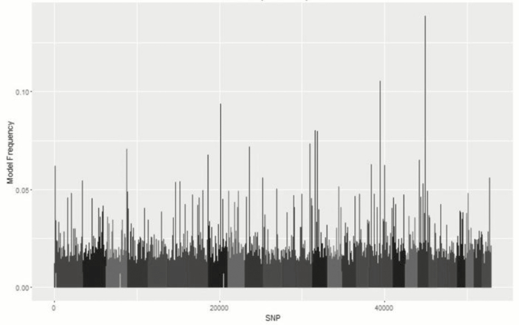
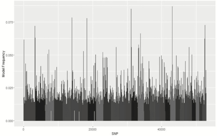
Metropolis plots of the model frequency of each SNP or haplotype loci across the genome for BayesC, BayesIM8, and BayesIM16 for ADG are in Figures 1 and 2, respectively. The model frequency of the SNP model begins at zero due to monomorphic SNP being included in the analysis but being excluded from models selected by BayesC. The magnitude of the model frequencies differed between models. As the number of covariates fitted at a given loci increased, the magnitude of the model frequency decreased resulting in the SNP analysis having higher model frequencies than BayesIM8 and BayesIM16. BayesIM8 also has higher model frequencies than BayesIM16 again due to half as many covariates being fitted at a given locus.

Figure 1.

Genome-wide association analysis between SNP genotypes and ADG from BayesC. The Y-axis represents the model frequency of each marker. On the X-axis, alternate gray scales represent different chromosomes from BTA 1 to BTA 29.

Figure 2.

Genome-wide association analysis between haplotype genotypes and ADG from BayesIM 8 (left) and BayesIM 16 clusters (right). The Y-axis represents the model frequency of each haplotype loci. On the X-axis, alternate gray scales represent different chromosomes from BTA 1 to BTA 29.

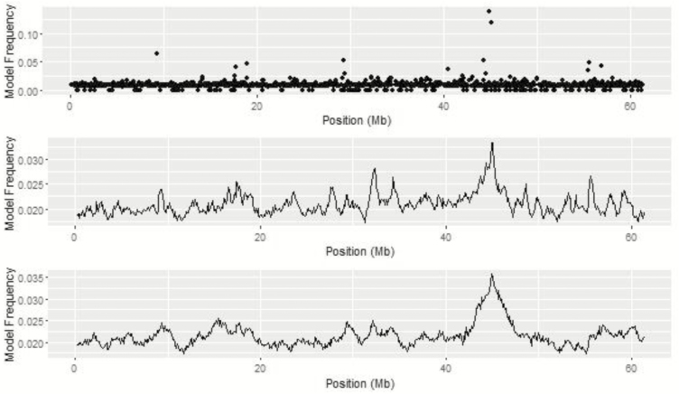
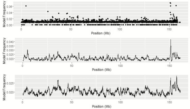
For ADG, a peak on BTA 22 is seen across all univariate analyses based on model and window frequency (Figure 3). The top SNP on BTA 22 was BTA-54550-no-rs at 44.94 Mb identified through the BayesC analysis. A second SNP with high model frequency, ARS-BFGL-NGS-81286, was nearby at 45.12 Mb. The maximum point of the QTL peak was at 45.0 Mb for both BayesIM8 and BayesIM16. The width of the QTL peak was defined as the position when the model frequency was greater than the mean model frequency of the chromosome and ends when the model frequency returns to the mean. The peak surrounding the top QTL on BTA 22 ranged from 40.54 to 46.68 Mb and 42.31 to 47.65 Mb for BayesIM8 and BayesIM16, respectively.

Figure 3.

BTA 22 from genome-wide association analyses for ADG from BayesC (top), BayesIM 8 clusters (middle), and BayesIM 16 clusters (bottom). The Y-axis represents the model frequency of each marker or haplotype loci. The X-axis is position in megabases (Mb) on BTA 22.

Gene ontology results for the extended 1-Mb window on BTA 22 include positive regulation of lipid formation (ABHD6), skeletal muscle tissue development (E1BKX7), muscle contraction (SLMAP), metabolic processes (LOC100847355), and regulation of glucose (APPL1). Snelling et al. (2011) discovered one significant SNP associated with ADG and two significant SNP associated with midtest metabolic weight (MMBW) in the adjacent region from 45 to 46 Mb on BTA 22. Within the same 1-Mb region, Bolormaa et al. (2011) found two additional SNP associated with MMBW.

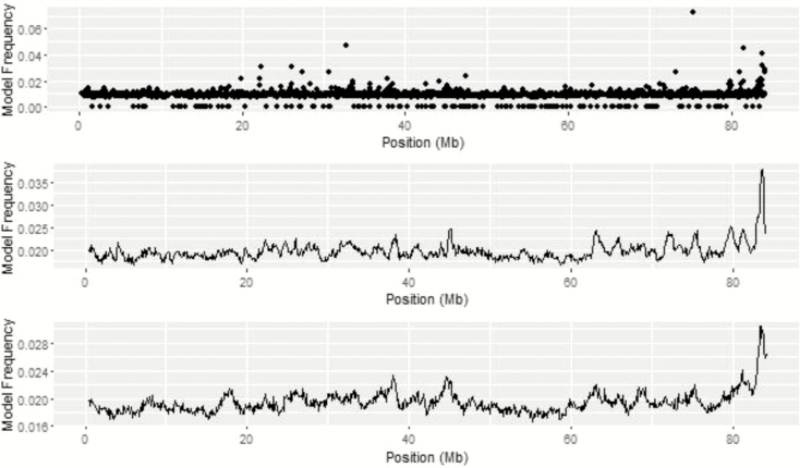
The QTL peak within the chromosomal region on BTA 13 from 83 to 84 Mb was common among the top 1% of 1-Mb windows across all univariate ADG analyses (Figure 4). While the top SNP based on model frequency on BTA 13 was at 75.27 Mb, two SNP within the region of interest, ARS-BFGL-NGS-114977 and ARS-BFGL-NGS-87042, were located at 83.80 and 83.76 Mb, respectively. The maximum of the QTL peak was at 83.7 Mb from BayesIM8 while it shifted slightly to 83.8 Mb for BayesIM16. The QTL region spanned from 81.93 Mb to the end of BTA 13 and from 79.21 Mb to the end of the chromosome for BayesIM8 and BayesIM16, respectively. Within this region are genes associated with the perception of smell (LOC532472) and nervous system development (DOK5). Lu et al. (2013) found ARS-BFGL-NGS-87042 to have a significant allelic substitution effect on DMI. An additional SNP in the same region, ARS-BFGL-NGS-89423, had a significant effect on birth weight (Lu et al., 2013).

Figure 4.

BTA 13 from genome-wide association analyses for ADG from BayesC (top), BayesIM 8 clusters (middle), and BayesIM 16 clusters (bottom). The Y-axis represents the model frequency of each marker or haplotype loci. The X-axis is position in megabases (Mb) on BTA 13.

Also, common across univariate analyses for ADG was BTA 3 from 119 to 120 Mb (Figure 5). The top SNP based on model frequency, ARS-BFGL-NGS-57851, was located at 119.55 Mb. The maximum point of the QTL peak was observed at 119.7 Mb from BayesIM8 and spanned from 118.62 to 121.94 Mb. When 16 haplotype clusters were assumed, the maximum point remained at 119.7 Mb and the width of the QTL peak decreased, 118.42 to 120.91 Mb. This region contains genes that are involved in cell proliferation (HDAC4), skeletal system development (HDAC4), metabolic processes (LOC782114), regulation of insulin and glucose (CAPN10), and positive regulation of skeletal muscle differentiation (GCP1). Serão et al. (2013) identified one SNP associated with residual ADG at 120.79 Mb.

Figure 5.

BTA 3 from genome-wide association analyses for ADG from BayesC (top), BayesIM 8 clusters (middle), and BayesIM 16 clusters (bottom). The Y-axis represents the model frequency of each marker or haplotype loci. The X-axis is position in megabases (Mb) on BTA 3.

Genomic Regions Associated With ADFI

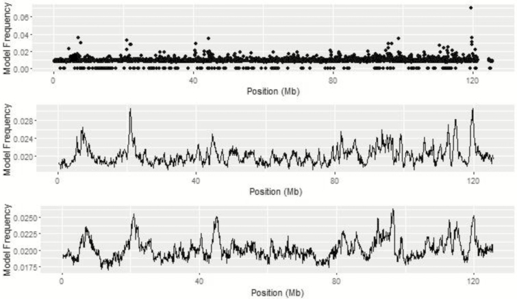
Metropolis plots for ADFI for BayesC, BayesIM8, and BayesIM16 are presented in Figures 6 and 7, respectively. The region from 151 to 152 Mb on BTA 1 was common across univariate analyses for ADFI based on model and window frequency (Figure 8). Three SNP with top model frequencies were within this window, ARS-BFGL-NGS-14751, ARS-BFGL-NGS-57499, and ARS-BFGL-NGS-70523, located at 151.00, 151.15, and 151.13 Mb, respectively. The haplotype analyses agreed with the maximum of the QTL peak located at 151.1 Mb from BayesIM8 and BayesIM16. Within this region, there were two peaks; a sharp, narrow QTL region followed by a broader area that began approximately 1 Mb following the tail of the first peak. For BayesIM8, the first peak ranged from 149.96 to 151.54 Mb with the subsequent interval starting at 152.48 Mb and extending to 156.04 Mb. When the number of haplotype clusters assumed increased, the range of the first peak was consistent (149.92 to 151.53 Mb), while the second QTL interval spanned nearly 8 Mb from 152.53 to 160.08 Mb. The region from 150.5 to 158.5 Mb spans across the two pronounced peaks on BTA 1.

Figure 6.

Genome-wide association analysis between SNP genotypes and ADFI from BayesC. The Y-axis represents the model frequency of each marker. On the X-axis, alternate gray scales represent different chromosomes from BTA 1 to BTA 29.

Figure 7.

Genome-wide association analysis between haplotype genotypes and ADFI from BayesIM 8 (left) and BayesIM 16 (right) clusters. The Y-axis represents the model frequency of each haplotype loci. On the X-axis, alternate gray scales represent different chromosomes from BTA 1 to BTA 29.

Figure 8.

BTA 1 from genome-wide association analyses for ADFI from BayesC (top), BayesIM 8 clusters (middle), and BayesIM 16 clusters (bottom). The Y-axis represents the model frequency of each marker or haplotype loci. The X-axis is position in megabases (Mb) on BTA 1.

At the frontend of this region, Lu et al. (2013) found a SNP located at 149.55 Mb to have a significant allelic substitution effect on ADG. At the end of the QTL peak at 157.50 Mb, the same authors found BTB-01633159 to be associated with residual feed intake (RFI). Gene ontology results for the extended window on BTA 1 include nervous system development (SIM2), cell proliferation (HLCS, RIPPLY3), and cell differentiation (ERG).

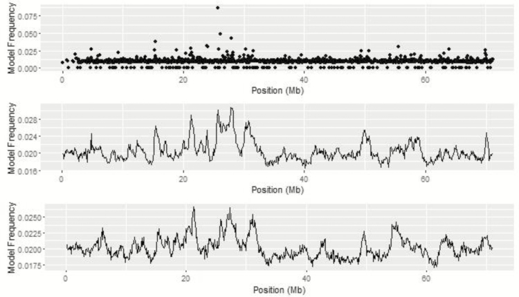
On BTA 21, the window from 27 to 28 Mb was associated with ADFI (Figure 9). Three SNP, Hapmap53212-rs29015272, BTB-01168615, and Hapmap49382-BTA-9378, were located at 25.70, 26.12 and 27.89 Mb, respectively. These top SNP were potentially in LD with the same QTL as the QTL window ranged from 25.19 to 29.23 Mb from BayesIM8 and 25.32 to 28.84 Mb from BayesIM16. Within this region, gene ontology results include positive regulation of cell proliferation (CTSH, RASGRF1) and metabolic processes (FAH, ABHD17C). Abo-Ismail et al. (2014) found two SNP with significant associations with RFI and one SNP significantly associated with DMI on BTA 21 near 29 Mb.

Figure 9.

BTA 21 from genome-wide association analyses for ADFI from BayesC (top), BayesIM 8 clusters (middle), and BayesIM 16 clusters (bottom). The Y-axis represents the model frequency of each marker or haplotype loci. The X-axis is position in megabases (Mb) on BTA 21.

Potential Pleiotropic Genomic Regions Associated With ADG and ADFI

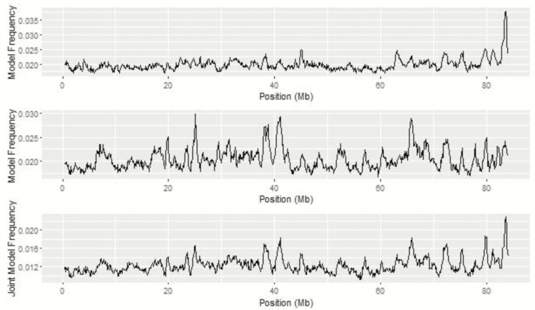
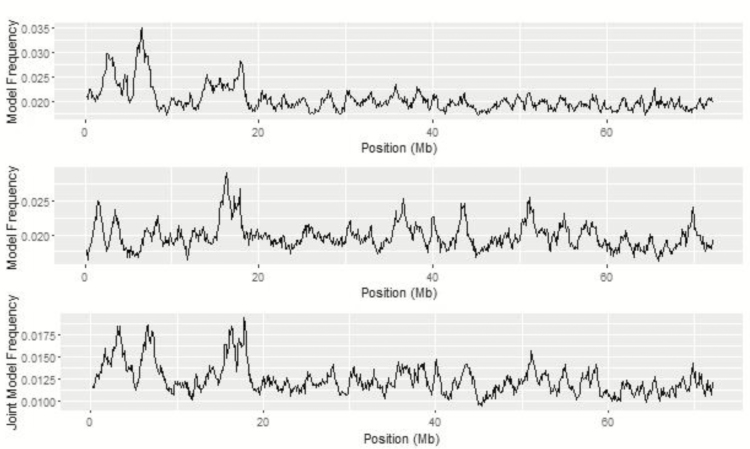
In the bivariate analyses, top regions identified have the potential to influence both traits. Metropolis plots of BayesIM8 bivariate and BayesIM16 bivariate are in Figure 10. It was expected that top regions in common across traits from the univariate analyses would also be apparent in the bivariate associations. The previously discussed region on BTA 13 was also identified in the top 1% of 1-Mb windows from haplotype bivariate associations. Comparison of QTL peaks from BayesIM8 for ADG, ADFI, and bivariate associations for BTA 13 are in Figure 11. Both univariate analyses and the bivariate analyses performed similar with all QTL intervals beginning at approximately 80 Mb and extending to the end of BTA 13.

Figure 10.

Genome-wide association analysis between haplotype genotypes and ADG and ADFI from BayesIM bivariate 8 (left) and BayesIM bivariate 16 clusters (right). The Y-axis represents the joint model frequency of each haplotype loci when both traits are included in the model. On the X-axis, alternate gray scales represent different chromosomes from BTA 1 to BTA 29.

Figure 11.

Comparison of univariate ADG (top) and ADFI (middle), and bivariate (bottom) haplotype associations for BTA 13 from BayesIM 8 clusters. The Y-axis represents the model frequency of each haplotype loci or the joint model frequency when both traits are in the model. The X-axis is position in megabases (Mb) on BTA 13.

The regions on BTA 20 from 4 to 5 Mb and 6 to 7 Mb were observed in the majority of bivariate analyses. Two QTL peaks spanned across these for both bivariate analyses with the first interval stretching from 0.40 to 4.84 Mb and the second interval spanning from 5.44 to 8.40 Mb from BayesIM8. When 16 clusters were assumed, a similar pattern was observed with the first interval ranging from 1.32 to 4.71 Mb and the second spanning from 5.98 to 7.64 Mb. This peak was observed in the univariate haplotype analysis for ADG. The interval locations were similar to the bivariate analyses ranging from 1.14 to 4.94 Mb and 5.22 to 8.05 Mb for BayesIM8 and 2.10 to 12.02 Mb for BayesIM16 for ADG. Comparison of genomic regions across univariate and bivariate haplotype analyses on BTA 20 are illustrated in Figure 12.

Figure 12.

Comparison of univariate ADG (top) and ADFI (middle), and bivariate (bottom) haplotype associations for BTA 20 from BayesIM 8 clusters. The Y-axis represents the model frequency of each haplotype loci or the joint model frequency when both traits are in the model. The X-axis is position in megabases (Mb) on BTA 20.

This region is flanked by two large-effect pleiotropic QTL discovered by Saatchi et al. (2014). A QTL associated with RFI and MMBW in a Hereford population was identified in the 1-Mb window from 4 to 5 Mb on BTA 20. The same study identified a significant window on BTA 20 from 8 to 9 Mb associated with ADG in an admixed population of beef cattle and MMBW in a Simmental × Angus population. Genes within this region are involved in metabolic processes (ENSBTAG00000015512, ENSBTAG00000034138) and fat cell differentiation (MSX2).

Although bivariate analyses detect genomic regions that are potentially associated with two traits, it is unknown if these regions are pleiotropic. Caution must be taken when interpreting genetic correlations between complex traits when conducting associations with molecular markers as linkage between markers can create phantom correlations between traits (Gianola et al., 2015).

CONCLUSIONS

Moving toward the use of haplotype models for genomic association studies has the ability to define the QTL locations more precisely. The traditional method of fitting SNP genotypes as covariates relies on LD between the marker and QTL. The corresponding location is that of the marker instead of the actual QTL of interest. Haplotype models allow for a QTL interval to be established with more resolution, which may help identify the casual variant when studies are advanced for fine mapping although the rank of MBV appears to be unaffected.

Multitrait GWAS is currently unexplored in the beef cattle industry. The deployment of such association studies would not only allow for the identification of potential pleiotropic regions, but offer a more comprehensive biological investigation into genetic variants affecting feed efficiency. Although not the case in this study, animals with missing phenotypic records can be included in the analysis. In beef cattle systems, gain is recorded frequently while feed intake is an expensive phenotype to collect. Since a moderate-to-strong genetic correlation exists between ADG and ADFI, it is logical to exploit the knowledge of one trait to inform the other.

LITERATURE CITED

- Abo-Ismail M. K., Vander Voort G., Squires J. J., Swanson K. C., Mandell I. B., Liao X., Stothard P., Moore S., Plastow G., and Miller S. P.. 2014. Single nucleotide polymorphisms for feed efficiency and performance in crossbred beef cattle. BMC Genet. 15:14. doi:10.1186/1471-2156-15-14 [DOI] [PMC free article] [PubMed] [Google Scholar]
- Arthur P. F., Archer J. A., Johnston D. J., Herd R. M., Richardson E. C., and Parnell P. F.. 2001a. Genetic and phenotypic variance and covariance components for feed intake, feed efficiency, and other postweaning traits in angus cattle. J. Anim. Sci. 79:2805–2811. doi:10.2527/2001.79112805x [DOI] [PubMed] [Google Scholar]
- Arthur P. F., Renand G., and Krauss D.. 2001b. Genetic and phenotypic relationships among different measures of growth and feed efficiency in young Charolais bulls. Livest. Prod. Sci. 68:131–139. doi:10.1016/S0301- 6226(00)00243-8 [Google Scholar]
- Bolormaa S., Hayes B. J., Savin K., Hawken R., Barendse W., Arthur P. F., Herd R. M., and Goddard M. E.. 2011. Genome-wide association studies for feedlot and growth traits in cattle. J. Anim. Sci. 89:1684–1697. doi:10.2527/jas.2010-3079 [DOI] [PubMed] [Google Scholar]
- Dickerson G. E., Kunzi N., Cundiff L. V., Koch R. M., Arthaud V. H., and Gregory G. E.. 1974. Selection criteria for efficient beef production. J. Anim. Sci. 39:659–673. doi:10.2527/jas1974.394659x [Google Scholar]
- FASS 1999. Guide for the care and use of agriculture animals in agriculture research and teaching http://www.fass.org/docs/agguide/Contents.pdf.
- Fernando R. L., and Garrick D. J.. 2009. GenSel user manual for a portfolio of genomic selection related analysis. Animal breeding and genetics. Iowa State University, Ames. [Google Scholar]
- Fox D. G., Tedeschi L. O., and Guiroy P. J.. 2001. Determining feed intake and feed efficiency of individual cattle fed in groups. Proc. Beef Improvement Federation Conference; July 11 to 14, 2001; San Antonio, TX p. 80–98. [Google Scholar]
- Freetly H. C., and Brown-Brandl T. M.. 2013. Enteric methane production from beef cattle that vary in feed efficiency. J. Anim. Sci. 91:4826–4831. doi:10.2527/jas.2011-4781 [DOI] [PubMed] [Google Scholar]
- Gianola D., de los Campos G., Toro M. A., Naya H., Schön C. C., and Sorensen D.. 2015. Do molecular markers inform about pleiotropy?Genetics 201:23–29. doi:10.1534/genetics.115.179978 [DOI] [PMC free article] [PubMed] [Google Scholar]
- Habier D., Fernando R. L., Kizilkaya K., and Garrick D. J.. 2011. Extension of the Bayesian alphabet for genomic selection. BMC Bioinformatics 12:186. doi:10.1186/1471-2105-12-186 [DOI] [PMC free article] [PubMed] [Google Scholar]
- Kachman S. D. 2016. Genomic prediction using a model based on haplotype clusters. J. Anim. Sci. 94 (Suppl. 2):16. [Google Scholar]
- Koch R. M., Swinger L. A., Chambers D., and Gregory K. E.. 1963. Efficiency of feed use in beef cattle. J. Anim. Sci. 22:486–494. doi:10.2527/jas1963.222486x [Google Scholar]
- Lu D., Miller S., Sargolzaei M., Kelly M., Vander Voort G., Caldwell T., Wang Z., Plastow G., and Moore S.. 2013. Genome-wide association analyses for growth and feed efficiency traits in beef cattle. J. Anim. Sci. 91:3612–3633. doi:10.2527/jas.2012-5716 [DOI] [PubMed] [Google Scholar]
- Nkrumah J. D., Basarab J. A., Wang Z., Li C., Price M. A., Okine E. K., Crews D. H. Jr, and Moore S. S.. 2007. Genetic and phenotypic relationships of feed intake and measures of efficiency with growth and carcass merit of beef cattle. J. Anim. Sci. 85:2711–2720. doi:10.2527/jas.2006-767 [DOI] [PubMed] [Google Scholar]
- Robinson D. L., and Oddy V. H.. 2004. Genetic parameters for feed efficiency, fatness, muscle area and feeding behaviour of feedlot finished beef cattle. Livest. Prod. Sci. 90:255–270. doi:10.1016/j.livprodsci.2004.06.011 [Google Scholar]
- Saatchi M., Beever J. E., Decker J. E., Faulkner D. B., Freetly H. C., Hansen S. L., Yampara-Iquise H., Johnson K. A., Kachman S. D., Kerley M. S.,. et al. 2014. QTLs associated with dry matter intake, metabolic mid-test weight, growth and feed efficiency have little overlap across 4 beef cattle studies. BMC Genomics 15:1004. doi:10.1186/1471-2164-15-1004 [DOI] [PMC free article] [PubMed] [Google Scholar]
- Schenkel F. S., Miller S. P., and Wilton J. W.. 2004. Genetic parameters and breed differences for feed efficiency, growth, and body composition traits of young beef bulls. Can. J. Anim. Sci. 84:177–185. doi:10.4141/A03-085 [Google Scholar]
- Serão N. V., González-Peña D., Beever J. E., Faulkner D. B., Southey B. R., and Rodriguez-Zas S. L.. 2013. Single nucleotide polymorphisms and haplotypes associated with feed efficiency in beef cattle. BMC Genet. 14:94. doi:10.1186/1471-2156-14-94 [DOI] [PMC free article] [PubMed] [Google Scholar]
- Snelling W. M., Allan M. F., Keele J. W., Kuehn L. A., Thallman R. M., Bennett G. L., Ferrell C. L., Jenkins T. G., Freetly H. C., Nielsen M. K.,. et al. 2011. Partial-genome evaluation of postweaning feed intake and efficiency of crossbred beef cattle. J. Anim. Sci. 89:1731–1741. doi:10.2527/jas.2010-3526 [DOI] [PubMed] [Google Scholar]
- Wilson-Wells D. F., and Kachman S. D.. 2016. A Bayesian GWAS method utilizing haplotype clusters for a composite breed population. Annual Conference on Applied Statistics in Agriculture; May 1 to 3, 2016; Manhattan, KS. [Google Scholar]
- Zimin A. V., Delcher A. L., Florea L., Kelley D. R., Schatz M. C., Puiu D., Hanrahan F., Pertea G., Van Tassell C. P., Sonstegard T. S.,. et al. 2009. A whole-genome assembly of the domestic cow, Bos taurus. Genome Biol. 10:R42. doi:10.1186/gb-2009-10-4-r42 [DOI] [PMC free article] [PubMed] [Google Scholar]