The Successor Representation: Its Computational Logic and Neural Substrates

Abstract

Reinforcement learning is the process by which an agent learns to predict long-term future reward. We now understand a great deal about the brain's reinforcement learning algorithms, but we know considerably less about the representations of states and actions over which these algorithms operate. A useful starting point is asking what kinds of representations we would want the brain to have, given the constraints on its computational architecture. Following this logic leads to the idea of the successor representation, which encodes states of the environment in terms of their predictive relationships with other states. Recent behavioral and neural studies have provided evidence for the successor representation, and computational studies have explored ways to extend the original idea. This paper reviews progress on these fronts, organizing them within a broader framework for understanding how the brain negotiates tradeoffs between efficiency and flexibility for reinforcement learning.

Introduction

Reinforcement learning, the problem of predicting and maximizing future reward, is hard in part because the number of possible futures is enormous, too big to search through exhaustively. A prospective student choosing between colleges cannot consider all possible career paths she might follow. She could try to learn from experience, picking a college and exploring the consequences, but she probably cannot do that enough times to find the optimal college. She could plan forward, at each decision point mentally choosing the option that seems most promising (“First I'll go to City University, then I'll major in chemistry, then I'll get a job at a pharmaceutical company, etc.”), or she could plan backward, starting from her goal (e.g., being rich, famous, etc.). But planning could go wrong if you explore the wrong path (if only I had majored in computer science instead of chemistry!). Yet another approach is to again imagine the goal state, but instead of planning a path to the goal, only consider how often the goal is achieved from a particular starting point (e.g., how many students who attend City University go on to become pharmaceutical chemists?). If she can access such statistics, then the prospective student could efficiently identify the best college.

As this example illustrates, the success of reinforcement learning algorithms hinges crucially on their representation of the environment. A very flexible representation, such as knowing how often each state transitions to every other state (e.g., the probability of getting a pharmaceutical job after graduating with a chemistry degree), can be highly accurate, but is computationally cumbersome—planning requires significant mental effort. On the other hand, a very inflexible representation, such as the summary of how good each college is based on past experience, is efficient (no planning required) but may be useless if the environment changes (e.g., the pharmaceutical industry crashes). A predictive summary statistic like how many students get jobs as chemists can be both flexible and efficient under certain circumstances (e.g., knowing that students at City University get jobs as chemists is useful if chemistry salaries suddenly increase).

Different representations clearly have different strengths and weaknesses. Computational models can help us to understand these tradeoffs in terms of general principles, guiding us toward answering a fundamental question: what makes a representation useful for reinforcement learning? This question is timely for the neuroscientific study of reinforcement learning, which has uncovered a rich and sometimes unruly menagerie of algorithms and representations. One lesson from these discoveries is that reinforcement learning is not one thing, but rather multiple things; a set of semi-dissociable “systems” that each can solve the reinforcement learning problem independently (Dolan and Dayan, 2013; Kool et al., 2018). These systems make different tradeoffs between computational efficiency and flexibility (Fig. 1), as elaborated in the next section. By formalizing this tradeoff space, we can clarify what makes a “good” representation for a given computational architecture.

Figure 1.

Schematic of how different reinforcement learning systems balance the efficiency-flexibility tradeoff. The efficiency axis represents the degree to which the computational architecture requires costly versus cheap computation. The flexibility axis represents the degree to which the architecture supports flexible adaptation to changes in the environment: how much new data needs to be gathered in order for value estimates to converge to the right answer. Not all of the algorithms listed in this figure are discussed in the text; see Gershman and Daw (2017) for a treatment of episodic reinforcement learning and Dayan et al. (2006) for a treatment of Pavlovian reinforcement learning.

Within this general framework, we will focus on a recently revived idea about how to balance efficiency and flexibility, known as the successor representation (SR; Dayan, 1993). The basic idea is to build a “predictive map” of the environment that summarizes the long-range predictive relationships between states of the environment. We will show how this predictive map, when used as the representation for reinforcement learning, is optimal for a particular computational architecture (linear function approximation). Recent experiments have begun to suggest that the SR may constitute part of a separate system for reinforcement learning, with implications for how we understand the functions of the hippocampus and dopamine.

An efficiency-flexibility tradeoff for reinforcement learning

Reinforcement learning is concerned with the estimation of value, the total reward an agent expects to earn in the future, with short-term rewards weighed more highly than long-term rewards. Formally, value is defined as the expected discounted future return (Sutton and Barto, 1998):

where s denotes the state of the environment, r_t denotes the reward received at time t, and γ is a discount factor that captures a preference for proximal rewards. The expectation 𝔼[·] represents an average over randomness in state transitions and rewards (i.e., transitions and rewards may be probabilistic, causing randomness in the sequence of experienced rewards). For simplicity of exposition, we have chosen to omit actions, though our treatment extends straightforwardly to handle actions (Russek et al., 2017).

To render the reinforcement learning problem tractable, it is common to make the additional assumption that transitions and rewards are governed by a Markov process, which means that rewards and state transitions depend only on the current state, regardless of the antecedent history. Formally, this corresponds to the assumption that 𝔼[r_t] = R(s_t) and P(s_t+1|s_t) = T(s_t, s_t+1), where R is referred to as the reward function and T is referred to as the transition function. Under this assumption, tractable algorithms can be derived for value function estimation, as described in detail by Sutton and Barto (1998).

Model-based algorithms, such as value iteration and Monte Carlo tree search, learn the underlying “model” (i.e., the reward function R and the transition function T), and use this model to compute an estimate of the value function by iterative computation. For example, value iteration repeatedly iterates the following update:

which will eventually converge to the true value function. Intuitively, value iteration starts with a guess about the value function, and iteratively refines this guess by enforcing consistency between the values of adjacent states. This architecture is computationally expensive, because value estimation must iterate over the entire state space each time the model is updated. The advantage of such an architecture lies in its flexibility: local changes in the environment lead to local changes in the model, and thus an agent endowed with a model requires only a small amount of experience to adapt to such changes.

Model-based algorithms represent one extreme in the tradeoff between computational efficiency and representational flexibility (Fig. 1). On the other extreme are model-free algorithms, such as temporal difference learning, which directly estimate the value function V from experienced transitions and rewards, without learning a model. In the most frugal computational architecture, the estimated value function Ṽ is represented by a lookup table storing the estimates for each state. However, a lookup table strategy may fail when the number of states is large and experience is sparse. To allow for some generalization across states, a linear function approximation architecture assigns value as a weighted combination of state features (Fig. 2):

where w_d is the weight for feature d and f_d(s) is the activation of feature d. The temporal difference learning rule for updating the weights takes the following form:

where

is the temporal difference error. If the value function has been overestimated, δ_t will be negative and hence the weights for active features [f_d(s_t) > 0] will be decreased, whereas if the value function has been underestimated, δ_t will be positive and the weights for active features will be increased. Notice that temporal difference learning “bootstraps” its value estimates, using one estimate to improve another estimate. This is computationally efficient, but also causes inflexibility: a local change in the transition or reward functions will produce nonlocal changes in the value function, such that the entire value function needs to be relearned by temporal difference updates whenever the environment changes. In the absence of a model, this necessitates direct experience of state transitions and rewards.

Figure 2.

Illustration of how different reinforcement learning systems compute value in a simple maze with three states (s₁, s₂, s₃). The reward value associated with each state is denoted by R(s), and its value estimate is denoted by Ṽ(s). Transition probabilities are denoted by T(s, s′) and the successor representation is denoted by M(s, s′). The parameter γ denotes the discount factor. The model-free value function estimate is assumed (for illustration) to be a linear function of x and y spatial coordinates, where w_x denotes the weight for the x-coordinate.

The linear function approximation architecture described above has been widely used in neural models of reinforcement learning (Schultz et al., 1997; Daw and Touretzky, 2002; Ludvig et al., 2008; Gershman, 2017a), but it will fail for value functions that are nonlinear. This has prompted some models to adopt a nonlinear function approximation architecture (Schmajuk and DiCarlo, 1992; Mondragón et al., 2017), a strategy that has proven successful in some machine learning applications (Mnih et al., 2015). Even with nonlinear architectures, model-free algorithms are typically computationally cheaper than model-based architectures. The cost of this frugality is inflexibility: the values at different states are coupled together, which means that local changes in the environment will lead to nonlocal changes in the value function, and thus a model-free agent will have to revisit many states to update their values. Function approximation can sometimes mitigate this problem by enabling generalization across states, but it can also sometimes exacerbate the problem by aliasing states that have distinct values.

It is important to recognize that the appropriate choice of function approximation architecture depends strongly on the choice of representation. For example, it is well known that linear architectures cannot solve “exclusive-or” problems (known as “negative patterning” in the animal learning literature), such as learning that I like broccoli and ice cream but not broccoli ice cream, when the features are elemental (i.e., 1 feature for broccoli and 1 for ice cream). However, adding a conjunctive feature that encodes broccoli ice cream will allow a linear architecture to solve the problem. More generally, many machine learning algorithms attempt to solve complex nonlinear problems by mapping the inputs into a new feature space in which linear methods will work well (Schölkopf and Smola, 2002; Bengio, 2009). This perspective has also permeated computational neuroscience, informing our understanding of object recognition (DiCarlo and Cox, 2007) and motor control (Sussillo and Abbott, 2009).

We can also flip this around and ask: for a given choice of function approximation architecture, what is the optimal representation? Linear architectures are often viewed as a reasonable starting point, given their analytical tractability, computational simplicity, and semi-biological plausibility (Poggio and Bizzi, 2004). This leads us directly to the SR.

The computational logic of the successor representation

Although above we differentiated between the relative merits of linear versus nonlinear architectures, it turns out that any value function can be represented as a linear combination of “predictive” features (Dayan, 1993):

where M(s, s′) is the SR, defined as the discounted occupancy of state s′, averaged over trajectories initiated in state s. The SR can intuitively be thought of as a predictive map that encodes each state in terms of the other states that will be visited in the near future. It is “optimal” in the sense that a linear function approximation architecture can exactly represent the value function if the features correspond to the SR; i.e., f_d(s) = M(s,d), where d indexes states.

The SR is defined analogously to the value function; instead of cumulating rewards (as in the value function), the SR cumulates state occupancies. There also exists an analogy between learning algorithms. In temporal difference learning, the value estimate is updated using a reward prediction error (the discrepancy between observed and expected reward). A temporal difference learning algorithm can also be derived for the SR, where the error signal is the discrepancy between observed and expected state occupancy (Russek et al., 2017):

where 𝕀[·] = 1 if its argument is true, and 0 otherwise. Intuitively, this learning rule states that the expected occupancy for states that are visited more frequently than expected (positive prediction error) should be increased, whereas the expected occupancy for states that are visited less frequently than expected (negative prediction error) should be decreased. Notice that unlike the temporal difference error for value learning, the temporal difference error for SR learning is vector-valued, with one error for each successor state. It is also possible to define a linear function approximator for the SR, in which case there is one error for each feature (Gardner et al., 2018).

In terms of the efficiency-flexibility tradeoff, the SR lies somewhere in between model-based and model-free algorithms. On the one hand, it has comparable efficiency to model-free reinforcement learning with linear function approximation. On the other hand, it has some of the flexibility of a model-based algorithm, in the sense that changes in the reward function will immediately propagate to all the state values, because the reward function has been factored out of the expectation over future trajectories, which means that an agent does not need to average over states to update V(s) when only R(s) changes. Note, however, that this is not true of changes in the transition function: the SR is effectively a compiled form of the state transition statistics, much in the same way that the value function is a compiled form of the reward statistics. It is this compilation that confers both efficiency and inflexibility.

We next turn to the behavioral and neural evidence that the brain computes the SR and uses it for reinforcement learning.

Behavioral evidence

Animals and humans are capable of “goal-directed” behavior, nimbly adapting to changes in the environment or their internal states as they pursue their goals. For example, Adams (1982) showed that rats trained to press a lever for sucrose subsequently ceased lever pressing in an extinction test after the sucrose was separately paired with illness (thereby devaluing the sucrose reinforcer) in the absence of the lever. It is critical that the rats did not have the opportunity to relearn the value of lever pressing after the devaluation treatment, thus ruling out a purely model-free account of behavior. Similarly, the observation that animals can learn under a variety of circumstances without direct reinforcement, such as latent learning (Tolman, 1948), is difficult to reconcile with model-free learning. Rather, these experimental phenomena have been interpreted as evidence for model-based control (Daw et al., 2005). However, they are not, as it turns out, strongly diagnostic of model-based control: they can be alternatively explained by SR-based accounts (Russek et al., 2017).

Take, for example, latent learning, in which an animal is placed in a maze for several days without any reward, and then subsequently trained to navigate to a rewarded location in the maze. The key finding, first reported by Tolman (1948), is that animals are faster at learning in the rewarded phase if they were first pretrained without reward. The SR provides a natural account for this finding (Russek et al., 2017), because the SR can be learned during pretraining without direct reinforcement. Then, during the training phase, the reward function is updated and combined with the SR to compute values. Importantly, the reward function (unlike the value function) can be learned locally, and hence is more quickly learnable.

As noted in the previous section, the SR predicts a distinctive pattern of behavioral flexibility, with greater sensitivity to changes in reward structure than to changes in transition structure. Changes in reward structure are propagated immediately to the values, because the reward predictions are represented explicitly and locally (i.e., 1 reward prediction for each state). In contrast, changes in transition structure will only propagate gradually, because the SR discards the local transition structure: it does not represent the fact that one state follows another with some probability, only that one state will tend to occur sometime in the future more frequently than another. This means that the entire SR must be relearned when the transition structure changes. Momennejad et al. (2017) exploited this fact to design a highly diagnostic test of whether human reinforcement learning follows the predictions of an SR-based learning algorithm (Fig. 3).

Figure 3.

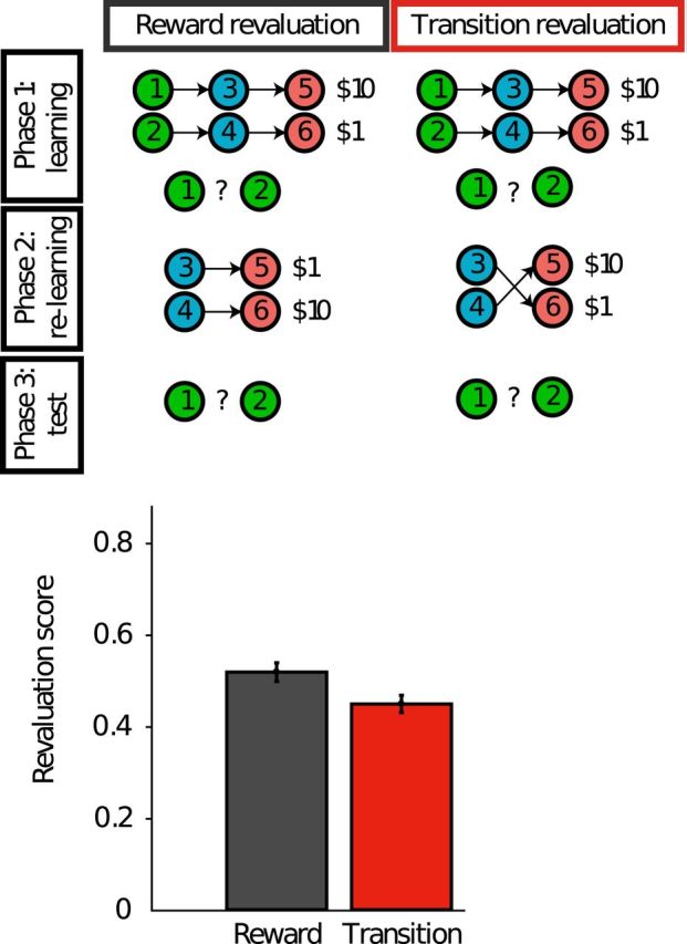
Top, Schematic of the experimental design used by Momennejad et al. (2017). Circles denote states and arrows denote transitions. The experiment consisted of three phases: learning, relearning, and test (in extinction). At the end of Phase 1 (learning) and Phase 3 (test), participants provided a continuous valued rating indicating which of the two starting states they preferred. Bottom, Revaluation score denotes the change in preference rating after versus before the relearning phase. Revaluation was significantly greater in the reward devaluation condition compared with the transition devaluation condition. Adapted from Momennejad et al. (2017).

The basic logic is the same as devaluation studies that have been used to study the goal-directedness of behavior in rodents (Dickinson, 1985) and humans (Valentin et al., 2007; Gershman et al., 2014). In the first phase, subjects first learned two chains of states (with different starting states) that lead to different amounts of reward. This differential reward was registered in subjects' preference for the starting state leading to the more rewarding terminal state. In the second phase, the task is altered, either by changing the reward structure (reward devaluation) or by changing the transition structure (transition devaluation). Both forms of devaluation alter the values of the initial states such that a reward-maximizing agent would reverse the preference learned in the first phase. Critically, subjects only experienced these changes starting in the intermediate states of each chain. This cripples temporal difference learning algorithms, which require unbroken sequences of states to learn correct values (but see Gershman et al., 2014). In the third phase, subjects were once again asked to choose between one of the starting states. Revaluation was measured as the difference in preference between the last and first phase (higher values indicating larger revaluation).

Based on the hypothesis that humans learn the SR with a temporal difference update rule, Momennejad et al. (2017) predicted, and confirmed, that revaluation would be greater in the reward devaluation condition compared with the transition devaluation condition (i.e., subjects reversed their preference more frequently in the reward revaluation condition), despite both changes having equivalent effects on the values of the starting states. The SR is able to rapidly adjust values in response to reward changes, thanks to the way in which the value function is parsed into predictive state and reward components. But this rapid adjustment is not enjoyed by the SR, under the assumption that it is updated using temporal difference learning. Interestingly, however, subjects were able to exhibit some zero-shot revaluation in the transition devaluation condition, despite the fact that temporal difference learning of the SR predicts that no revaluation should occur. Model comparison suggested that subjects were using a combination of SR-based and model-based strategies, whereby the SR provides an initial estimate of the value function, which is then refined by model-based computation. This kind of “cooperative” interplay between reinforcement learning systems has been observed in a number of experiments, realized in a variety of ways (for review, see Kool et al., 2018).

Neural evidence

Consider what the SR looks like in an open field with uniformly distributed rewards (Fig. 4). Because the agent is equally like to go in any direction, the SR for a given state (corresponding to a spatial location) will be radially symmetric over space, with a width that depends on the discount factor γ (larger values of γ translate to larger widths). If we now imagine a collection of neurons encoding this spatial function for each state, then the resulting population code will closely resemble classical place fields observed in the hippocampus (Stachenfeld et al., 2017).

Figure 4.

Place field corresponding to a single column of the successor representation. Left, States are organized into a two-dimensional spatial layout, where each state corresponds to a single (x, y) coordinate. Each state has can be represented in terms of the expected occupancy of all other states. These predictive representations can then be organized into a matrix (right), where each row corresponds to the successor representation of a particular state. A place cell's firing field corresponds to a single column of the matrix. Thus, the successor representation is encoded by the population of place cells. Approximately radially symmetric fields arise from random foraging in an open field.

Although the SR looks like a purely spatial code in the simple setting of random foraging, it takes on richer characteristics in more complex environments. For example, adding impassable barriers to the open field causes the SR to distort around the barrier (Stachenfeld et al., 2017), consistent with experimental observations (Muller and Kubie, 1987; Skaggs and McNaughton, 1998; Alvernhe et al., 2011). The SR can also explain why place cells become skewed opposite the direction of travel over the course of repeated traversals (Mehta et al., 2000). As the predictive representation is learned across a reliable state sequence, upcoming states become predictable further in advance. Place cells are also sensitive to nonspatial factors: place fields tend to cluster around rewarded locations (Hollup et al., 2001), which arises in the SR model because the animal tends to visit those states more frequently. Brain imaging studies in humans recapitulate these observations, indicating an important role for hippocampus in predictive representation (Schapiro et al., 2016; Garvert et al., 2017).

The SR model provides a bridge between these neural observations and animal learning data. For example, a well known finding in the contextual fear conditioning literature is the facilitatory effect of pre-exposure to a context (Fanselow, 2010). From the perspective of the SR, this is essentially a kind of latent learning: the animal develops a predictive representation that can then be used to generalize fear from one location in the conditioning apparatus to all others (Fig. 5). Importantly, hippocampal lesions cause a sharp reduction in the pre-exposure effect, consistent with the SR model's interpretation that this region encodes the predictive map.

Figure 5.

Left, Fear-related freezing response in rats following fear conditioning is stronger if the animal is pre-exposed to the conditioning environment. This effect is much weaker following hippocampal lesions. Adapted from Fanselow (2010). Right, Exploring the environment allows the hippocampus to learn a predictive representation, which can then be used to generalize value across states. Adapted from Stachenfeld et al. (2017).

An important question concerns how the SR is learned. What seems to be required, if we are to take the temporal difference learning story seriously, is a vector-valued error signal that conveys state (or sensory feature) prediction errors. One recent proposal argues that the phasic firing of midbrain dopamine neurons provides the necessary error signal (Gardner et al., 2018). This might seem heterodox for the conventional interpretation of phasic dopamine, according to which the firing rate conveys the temporal difference error for value updating (Eq. 5). However, a number of recent studies seem to contradict the “pure reward” interpretation of dopamine: (1) dopamine neurons respond to sensory prediction errors (Takahashi et al., 2017), (2) dopamine transients are necessary for learning driven by these errors (Chang et al., 2017), and (3) dopamine transients are both sufficient and necessary for learning stimulus–stimulus associations (Sharpe et al., 2017). Using simulations, Gardner et al. (2018) showed that all of these findings could be accounted for under the assumption that dopamine signals temporal difference errors for the SR.

Moving outside the temporal difference learning framework, it is also possible to learn the successor representation using biologically plausible plasticity rules, as shown by Brea et al., (2016). In particular, spike-timing-dependent plasticity can give rise to a form of prospective coding in which dendrites learn to anticipate future somatic spiking. Brea et al. (2016) showed that such prospective coding is mathematically equivalent to the SR, and is consistent with a number of neurophysiological observations. For example, in monkeys performing a delayed paired-associate task, some prefrontal neurons appear to ramp in anticipation of a predictable stimulus (Rainer et al., 1999).

Conclusions and future directions

What makes a good representation for reinforcement learning? There is no single answer to this question, because the goodness of a representation depends on the computational architecture in which it participates. To better understand this interplay, we analyzed different representational choices in terms of the tradeoff between efficiency (computational cost) and flexibility (how quickly the system adapts to changes in the environment). The brain appears to make use of multiple reinforcement learning systems that occupy different positions within this space (Kool et al., 2018). Importantly, each gain in efficiency is accompanied by a reduction in flexibility (Fig. 1).

For a linear function approximation architecture, we showed that the correct representation is the SR, in the sense that a perfectly learned SR will allow exact value computation. The SR occupies an intermediate position in the efficiency-flexibility space, with efficiency comparable to linear model-free methods and flexibility comparable to model-based methods. This and other computational properties have led to a recent resurgence of interest in the SR for machine learning (Kulkarni et al., 2016; Barreto et al., 2017; Zhang et al., 2017).

The research program reviewed in this paper is still in its infancy, and many questions remain. Here we highlight a few of these questions.

First, we have suggested that dopamine conveys a vector-valued signal for updating the SR (Gardner et al., 2018). This is completely speculative at this point, because no one has systematically investigated whether dopamine signals are vector-valued, except in limited and indirect ways. Ensemble recordings of dopamine neurons will be useful for a more decisive test of this hypothesis.

Second, the SR is unlikely to be a self-contained reinforcement learning system; empirical (Momennejad et al., 2017) and theoretical (Russek et al., 2017) arguments indicate that it interacts with both model-based and model-free computations. The nature of these interactions is still unclear, however. Once we have a more systematic mapping of computations onto brain structures, we may have better purchase on this question. For example, Momennejad et al. (2017) presented evidence suggesting that model-based computations incrementally refine an initial SR-based estimate of the value function. If this is true, then we should expect to see SR-related neural signals early on, which are later superseded by model-based neural signals. Another possibility is that the model-based system plans to some depth and then uses the SR to compute a heuristic value function (Keramati et al., 2016). Yet another possibility is that the SR provides an efficient search space for model-based planning, which can be implemented using attractor dynamics (Corneil and Gerstner, 2015).

Third, we have assumed that the value function approximation, at least the one that interfaces with the SR, is linear. Is that a reasonable assumption? This question is intrinsically hard to answer, because we do not know how to directly analyze the function approximation architecture used by a neural circuit. Most biologically realistic neural circuits are of course nonlinear, but the question is whether a linear model is a useful abstraction. As we learn more about the circuit computations underlying reinforcement learning, our assumptions about representation may change in tandem.

Fourth, we have assumed that the brain knows what state it is in, and moreover has some representation of the entire state space. But in reality we often have uncertainty about the underlying state (the state inference problem), and may also have uncertainty about the state space itself (the state discovery problem). These problems raise the question of how to think about the SR under state uncertainty. Some theories posit that the brain forms a posterior distribution over hidden states conditional on sensory data (Daw et al., 2006; Gershman et al., 2010; Rao, 2010; Soto et al., 2014; Babayan et al., 2018; Starkweather et al., 2018), in which case the SR would need to be defined over the continuous space of probability distributions. Although this is a well defined problem mathematically, it is an open question how the brain accomplishes this in a computationally tractable way.

Fifth, if the hippocampus encodes the SR, then we can make predictions about how it should respond to the transition and reward manipulations in revaluation experiments (Momennejad et al., 2017). Specifically, we would expect that when reward changes, the firing rates of hippocampal neurons should respond only once the animal's policy begins to change, because the animal will only observe changes in state occupancy when it alters its policy. In contrast, transition changes should cause hippocampal neurons to respond immediately (before any policy change) because of the altered state occupancy statistics.

Finally, a separate line of research has implicated the SR in memory (Gershman, 2017b). In particular, the SR is closely related to mathematical models of item–context associations (Gershman et al., 2012), and the temporal difference learning algorithm offers a new way of thinking about how these associations are updated (Smith et al., 2013; Manns et al., 2015). Presently, it is unclear whether memory and reinforcement learning rely on a common neural substrate, although the shared dependence on the hippocampus suggests this as a plausible conjecture.

References

- Adams CD. (1982) Variations in the sensitivity of instrumental responding to reinforcer devaluation. Q J Exp Psychol 34:77–98. 10.1080/14640748208400878 [DOI] [Google Scholar]
- Alvernhe A, Save E, Poucet B (2011) Local remapping of place cell firing in the tolman detour task. Eur J Neurosci 33:1696–1705. 10.1111/j.1460-9568.2011.07653.x [DOI] [PubMed] [Google Scholar]
- Babayan BM, Uchida N, Gershman SJ (2018) Belief state representation in the dopamine system. Nat Commun 9:1891. 10.1038/s41467-018-04397-0 [DOI] [PMC free article] [PubMed] [Google Scholar]
- Barreto A, Dabney W, Munos R, Hunt JJ, Schaul T, Van Hasselt H, Silver D (2017) Successor features for transfer in reinforcement learning. In: Advances in neural information processing systems, pp 4056–4066. Cambridge, MA: MIT. [Google Scholar]
- Bengio Y. (2009) Learning deep architectures for AI. Found Trends Mach Learn 2:1–127. 10.1561/2200000006 [DOI] [Google Scholar]
- Brea J, Gaál AT, Urbanczik R, Senn W (2016) Prospective coding by spiking neurons. PLoS Comput Biol 12:e1005003. 10.1371/journal.pcbi.1005003 [DOI] [PMC free article] [PubMed] [Google Scholar]
- Chang CY, Gardner M, Di Tillio MG, Schoenbaum G (2017) Optogenetic blockade of dopamine transients prevents learning induced by changes in reward features. Curr Biol 27:3480–3486.e3. 10.1016/j.cub.2017.09.049 [DOI] [PMC free article] [PubMed] [Google Scholar]
- Corneil DS, Gerstner W (2015) Attractor network dynamics enable preplay and rapid path planning in maze-like environments. In: Advances in neural information processing systems, pp 1684–1692. Cambridge, MA: MIT. [Google Scholar]
- Daw ND, Touretzky DS (2002) Long-term reward prediction in TD models of the dopamine system. Neural Comput 14:2567–2583. 10.1162/089976602760407973 [DOI] [PubMed] [Google Scholar]
- Daw ND, Niv Y, Dayan P (2005) Uncertainty-based competition between prefrontal and dorsolateral striatal systems for behavioral control. Nat Neurosci 8:1704–1711. 10.1038/nn1560 [DOI] [PubMed] [Google Scholar]
- Daw ND, Courville AC, Touretzky DS (2006) Representation and timing in theories of the dopamine system. Neural Comput 18:1637–1677. 10.1162/neco.2006.18.7.1637 [DOI] [PubMed] [Google Scholar]
- Dayan P. (1993) Improving generalization for temporal difference learning: the successor representation. Neural Comput 5:613–624. 10.1162/neco.1993.5.4.613 [DOI] [Google Scholar]
- Dayan P, Niv Y, Seymour B, Daw ND (2006) The misbehavior of value and the discipline of the will. Neural Netw 19:1153–1160. 10.1016/j.neunet.2006.03.002 [DOI] [PubMed] [Google Scholar]
- DiCarlo JJ, Cox DD (2007) Untangling invariant object recognition. Trends Cogn Sci 11:333–341. 10.1016/j.tics.2007.06.010 [DOI] [PubMed] [Google Scholar]
- Dickinson A. (1985) Actions and habits: the development of behavioural autonomy. Phil Trans R Soc Lond B Biol Sci 308:67–78. 10.1098/rstb.1985.0010 [DOI] [Google Scholar]
- Dolan RJ, Dayan P (2013) Goals and habits in the brain. Neuron 80:312–325. 10.1016/j.neuron.2013.09.007 [DOI] [PMC free article] [PubMed] [Google Scholar]
- Fanselow MS. (2010) From contextual fear to a dynamic view of memory systems. Trends Cogn Sci 14:7–15. 10.1016/j.tics.2009.10.008 [DOI] [PMC free article] [PubMed] [Google Scholar]
- Gardner MPH, Schoenbaum, Gershman SJ (2018) Rethinking dopamine prediction errors. bioRxiv 239731 10.1101/239731 [DOI] [PMC free article] [PubMed] [Google Scholar]
- Garvert MM, Dolan RJ, Behrens TE (2017) A map of abstract relational knowledge in the human hippocampal–entorhinal cortex. eLife 6:e17086. 10.7554/eLife.17086 [DOI] [PMC free article] [PubMed] [Google Scholar]
- Gershman SJ. (2017a) Dopamine, inference, and uncertainty. Neural Comput 29:3311–3326. 10.1162/neco_a_01023 [DOI] [PubMed] [Google Scholar]
- Gershman SJ. (2017b) Predicting the past, remembering the future. Curr Opin Behav Sci 17:7–13. 10.1016/j.cobeha.2017.05.025 [DOI] [PMC free article] [PubMed] [Google Scholar]
- Gershman SJ, Daw ND (2017) Reinforcement learning and episodic memory in humans and animals: an integrative framework. Annu Rev Psychol 68:101–128. 10.1146/annurev-psych-122414-033625 [DOI] [PMC free article] [PubMed] [Google Scholar]
- Gershman SJ, Blei DM, Niv Y (2010) Context, learning, and extinction. Psychol Rev 117:197–209. 10.1037/a0017808 [DOI] [PubMed] [Google Scholar]
- Gershman SJ, Moore CD, Todd MT, Norman KA, Sederberg PB (2012) The successor representation and temporal context. Neural Comput 24:1553–1568. 10.1162/NECO_a_00282 [DOI] [PubMed] [Google Scholar]
- Gershman SJ, Markman AB, Otto AR (2014) Retrospective revaluation in sequential decision making: a tale of two systems. J Exp Psychol Gen 143:182–194. 10.1037/a0030844 [DOI] [PubMed] [Google Scholar]
- Hollup SA, Molden S, Donnett JG, Moser MB, Moser EI (2001) Accumulation of hippocampal place fields at the goal location in an annular watermaze task. J Neurosci 21:1635–1644. 10.1523/JNEUROSCI.21-05-01635.2001 [DOI] [PMC free article] [PubMed] [Google Scholar]
- Keramati M, Smittenaar P, Dolan RJ, Dayan P (2016) Adaptive integration of habits into depth-limited planning defines a habitual-goal-directed spectrum. Proc Natl Acad Sci U S A 113:12868–12873. 10.1073/pnas.1609094113 [DOI] [PMC free article] [PubMed] [Google Scholar]
- Kool W, Cushman FA, Gershman SJ (2018) Competition and cooperation between multiple reinforcement learning systems. In: Goal-directed decision making: computations and neural circuits. New York: Academic. [Google Scholar]
- Kulkarni TD, Saeedi A, Gautam S, Gershman SJ (2016) Deep successor reinforcement learning. arXiv:1606.02396. [Google Scholar]
- Ludvig EA, Sutton RS, Kehoe EJ (2008) Stimulus representation and the timing of reward-prediction errors in models of the dopamine system. Neural Comput 20:3034–3054. 10.1162/neco.2008.11-07-654 [DOI] [PubMed] [Google Scholar]
- Manns JR, Galloway CR, Sederberg PB (2015) A temporal context repetition effect in rats during a novel object recognition memory task. Anim Cogn 18:1031–1037. 10.1007/s10071-015-0871-3 [DOI] [PubMed] [Google Scholar]
- Mehta MR, Quirk MC, Wilson MA (2000) Experience-dependent asymmetric shape of hippocampal receptive fields. Neuron 25:707–715. 10.1016/S0896-6273(00)81072-7 [DOI] [PubMed] [Google Scholar]
- Mnih V, Kavukcuoglu K, Silver D, Rusu AA, Veness J, Bellemare MG, Graves A, Riedmiller M, Fidjeland AK, Ostrovski G, Petersen S, Beattie C, Sadik A, Antonoglou I, King H, Kumaran D, Wierstra D, Legg S, Hassabis D (2015) Human-level control through deep reinforcement learning. Nature 518:529–533. 10.1038/nature14236 [DOI] [PubMed] [Google Scholar]
- Momennejad I, Russek EM, Cheong JH, Botvinick MM, Daw N, Gershman SJ (2017) The successor representation in human reinforcement learning. Nat Hum Behav 1:680–692. 10.1038/s41562-017-0180-8 [DOI] [PMC free article] [PubMed] [Google Scholar]
- Mondragón E, Alonso E, Kokkola N (2017) Associative learning should go deep. Trends Cogn Sci 21:822–825. 10.1016/j.tics.2017.06.001 [DOI] [PubMed] [Google Scholar]
- Muller RU, Kubie JL (1987) The effects of changes in the environment on the spatial firing of hippocampal complex-spike cells. J Neurosci 7:1951–1968. 10.1523/JNEUROSCI.07-07-01951.1987 [DOI] [PMC free article] [PubMed] [Google Scholar]
- Poggio T, Bizzi E (2004) Generalization in vision and motor control. Nature 431:768–774. 10.1038/nature03014 [DOI] [PubMed] [Google Scholar]
- Rainer G, Rao SC, Miller EK (1999) Prospective coding for objects in primate prefrontal cortex. J Neurosci 19:5493–5505. 10.1523/JNEUROSCI.19-13-05493.1999 [DOI] [PMC free article] [PubMed] [Google Scholar]
- Rao RP. (2010) Decision making under uncertainty: a neural model based on partially observable markov decision processes. Front Comput Neurosci 4:146. 10.3389/fncom.2010.00146 [DOI] [PMC free article] [PubMed] [Google Scholar]
- Russek EM, Momennejad I, Botvinick MM, Gershman SJ, Daw ND (2017) Predictive representations can link model-based reinforcement learning to model-free mechanisms. PLoS Comput Biol 13:e1005768. 10.1371/journal.pcbi.1005768 [DOI] [PMC free article] [PubMed] [Google Scholar]
- Schapiro AC, Turk-Browne NB, Norman KA, Botvinick MM (2016) Statistical learning of temporal community structure in the hippocampus. Hippocampus 26:3–8. 10.1002/hipo.22523 [DOI] [PMC free article] [PubMed] [Google Scholar]
- Schmajuk NA, DiCarlo JJ (1992) Stimulus configuration, classical conditioning, and hippocampal function. Psychol Rev 99:268–305. 10.1037/0033-295X.99.2.268 [DOI] [PubMed] [Google Scholar]
- Schölkopf B, Smola AJ (2002) Learning with kernels: support vector machines, regularization, optimization, and beyond. Cambridge, MA: MIT. [Google Scholar]
- Schultz W, Dayan P, Montague PR (1997) A neural substrate of prediction and reward. Science 275:1593–1599. 10.1126/science.275.5306.1593 [DOI] [PubMed] [Google Scholar]
- Sharpe MJ, Chang CY, Liu MA, Batchelor HM, Mueller LE, Jones JL, Niv Y, Schoenbaum G (2017) Dopamine transients are sufficient and necessary for acquisition of model-based associations. Nat Neurosci 20:735–742. 10.1038/nn.4538 [DOI] [PMC free article] [PubMed] [Google Scholar]
- Skaggs WE, McNaughton BL (1998) Spatial firing properties of hippocampal ca1 populations in an environment containing two visually identical regions. J Neurosci 18:8455–8466. 10.1523/JNEUROSCI.18-20-08455.1998 [DOI] [PMC free article] [PubMed] [Google Scholar]
- Smith TA, Hasinski AE, Sederberg PB (2013) The context repetition effect: predicted events are remembered better, even when they don't happen. J Exp Psychol Gen 142:1298–1308. 10.1037/a0034067 [DOI] [PubMed] [Google Scholar]
- Soto FA, Gershman SJ, Niv Y (2014) Explaining compound generalization in associative and causal learning through rational principles of dimensional generalization. Psychol Rev 121:526–558. 10.1037/a0037018 [DOI] [PMC free article] [PubMed] [Google Scholar]
- Stachenfeld KL, Botvinick MM, Gershman SJ (2017) The hippocampus as a predictive map. Nat Neurosci 20:1643–1653. 10.1038/nn.4650 [DOI] [PubMed] [Google Scholar]
- Starkweather CK, Gershman SJ, Uchida N (2018) The medial prefrontal cortex shapes dopamine reward prediction errors under state uncertainty. Neuron 98:616–629.e6. 10.1016/j.neuron.2018.03.036 [DOI] [PMC free article] [PubMed] [Google Scholar]
- Sussillo D, Abbott LF (2009) Generating coherent patterns of activity from chaotic neural networks. Neuron 63:544–557. 10.1016/j.neuron.2009.07.018 [DOI] [PMC free article] [PubMed] [Google Scholar]
- Sutton RS, Barto AG (1998) Reinforcement learning: an introduction. Cambridge, MA: MIT. [Google Scholar]
- Takahashi YK, Batchelor HM, Liu B, Khanna A, Morales M, Schoenbaum G (2017) Dopamine neurons respond to errors in the prediction of sensory features of expected rewards. Neuron 95:1395–1405.e3. 10.1016/j.neuron.2017.08.025 [DOI] [PMC free article] [PubMed] [Google Scholar]
- Tolman EC. (1948) Cognitive maps in rats and men. Psychol Rev 55:189–208. 10.1037/h0061626 [DOI] [PubMed] [Google Scholar]
- Valentin VV, Dickinson A, O'Doherty JP (2007) Determining the neural substrates of goal-directed learning in the human brain. J Neurosci 27:4019–4026. 10.1523/JNEUROSCI.0564-07.2007 [DOI] [PMC free article] [PubMed] [Google Scholar]
- Zhang J, Springenberg JT, Boedecker J, Burgard W (2017) Deep reinforcement learning with successor features for navigation across similar environments. In: IROS Vancouver 2017: IEEE/RSJ international conference on intelligent robots and systems: Vancouver, BC, Canada, September 24–28, 2017, pp 2371–2378. Piscataway, NJ: IEEE. [Google Scholar]