Post-Selection Inference for ℓ₁-Penalized Likelihood Models

Abstract

We present a new method for post-selection inference for ℓ₁ (lasso)-penalized likelihood models, including generalized regression models. Our approach generalizes the post-selection framework presented in Lee et al. (2013). The method provides p-values and confidence intervals that are asymptotically valid, conditional on the inherent selection done by the lasso. We present applications of this work to (regularized) logistic regression, Cox's proportional hazards model and the graphical lasso. We do not provide rigorous proofs here of the claimed results, but rather conceptual and theoretical sketches.

1 Introduction

Significant recent progress has been made in the problem of inference after selection for Gaussian regression models. In particular, Lee et al. (2013) derives closed form p-values and confidence intervals, after fitting the lasso with a fixed value of the regularization parameter, and Taylor et al. (2014) provides analogous results for forward stepwise regression and least angle regression (LAR). In this paper we derive a simple and natural way to extend these results to ℓ₁-penalized likelihood models, including generalized regression models such as (regularized) logistic regression and Cox's proportional hazards model.

Formally, the results described here are contained in Tian and Taylor (2015) in which the authors consider the same problems but having added noise to the data before fitting the model and carrying out the selection. Besides expanding on the GLM case, considered only briefly in Tian and Taylor (2015), the novelty in this work is the second-stage estimator, which is asymptotically equivalent to the post-LASSO MLE, and overcomes some problems encountered with a second-order remainder. And unlike the proposals in Tian and Taylor (2015), the estimator proposed here does not require MCMC sampling and is computable in closed form. Our estimator comprises of a single step of Newton-Raphson (or equivalently, Fisher scoring) in the selected model after having fit the LASSO. This is discussed further in Section 3. We note that one-step estimators are commonly used in semi-parametric inference: see for example Bickel et al. (1993).

In this paper we do not provide rigorous proofs of the claimed results, but rather theoretical and conceptual sketches, together with numerical evidence. We are confident that rigorous proofs can be given (with appropriate assumptions) and plan to report these elsewhere. We also note the strong similarity between our one-step estimator and the “debiased lasso” construction of Zhang and Zhang (2014), Bühlmann (2013), van de Geer et al. (2013), and Javanmard and Montanari (2014). This connection is detailed in Remark A of this paper.

Figure 1 shows an example, the South African heart disease data. This is a retrospective sample of 463 males in a heart-disease high-risk region of the Western Cape, South Africa. The outcome is binary— coronary heart disease— and there are 9 predictors. We applied lasso-penalized logistic regression, choosing the tuning parameter by cross-validation. The left panel shows the standard (naive) p-values and the post-selection p-values from our theory, for the predictors in the active set. Since the sample size is large compared to the number of predictors, the unadjusted and adjusted p-values are only substantially different for two of the predictors. On the right we have added 100 independent standard Gaussian predictors (labelled X1, X2 … X100) to examine the effects of selection. Now the naive p-values are unrealistically small for the noise variables while the adjusted p-values are appropriately large. Although our focus is on selection via ℓ₁-penalization, a similar approach can likely be applied to forward stepwise methods for likelihood models, and in principle, least angle regression (LAR).

Figure 1.

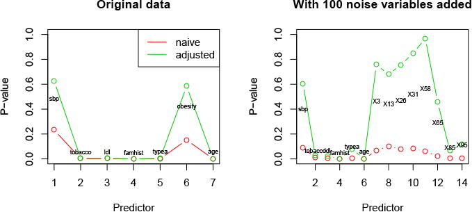
South African Heart disease data. P-values from naive and selection-adjusted approaches, for original data (left) and data with 100 additional noise predictors (right). Each model was chosen by lasso-penalized logistic regression, choosing the tuning parameter by cross-validation. The small p-values in the left panel are all below 0.001

An outline of this paper is as follows. Section 2 reviews post-selection inference for the lasso in the Gaussian regression model and introduces our proposal for more general (non-Gaussian) generalized linear models. In Section 3 we give an equivalent form of the proposal, one that applies to general likelihood models, for example the graphical lasso. We give a rough argument for the asymptotic validity of the procedure. Section 4 reports a simulation study of the methods. In Section 5 we show an example of the proposal applied to Cox's model for survival data. The graphical lasso is studied in Section 6. We end with a discussion in Section 7.

2 Post-selection inference for generalized regression models

Suppose that we have data (x_i, y_i), i = 1, 2, … N consisting of features x_i = (x_i1, x_i2, … x_ip) and outcomes y_i, i = 1, 2, … N. Let X = {x_ij} be the N × p data matrix. We consider a generalized regression model with linear predictor η = α + x^T β and log-likelihood ℓ(α, β). Our objective function has the form

$$J(\alpha ,\beta )=-\ell (\alpha ,\beta )+\lambda \cdot \sum _1^p\left|{\beta }_j\right|.$$ (1)

Let α̂, β̂ be the minimizers of J(α, β). We wish to carry out selective inference for some functional γ^T β. For example, γ might be chosen so that γ^T β is the population partial regression coefficient for the jth predictor.

As a leading example, we consider the logistic regression model specified by

$$\begin{array}{l}\pi =E(Y|x);log\pi /(1-\pi )=\alpha +x^T\beta ;\\ \ell (\alpha ,\beta )=\sum [y_{i}log({\pi }_i)+(1-y_i)log(1-{\pi }_i)].\end{array}$$ (2)

Having fit this model using a fixed value of λ, we carry out post-selection inference, as in the heart disease example above.

The reader may well ask: “partial regression coefficient with respect to what?”, i.e. what other covariates are we going to control for? In this paper, we follow the selected model framework described in Fithian et al. (2014) so that having observed M, the sparsity pattern of β̂ as returned by the LASSO, we carry out selective inference for linear functionals of β_M ∈ ℝ^M under the assumption that the model (2) is correct with parameter β* satisfying β*_−M = 0. That is, we carry out selective inference under the assumption that the LASSO has screened successfully, at least approximately.

There are various ways we might modify this model, though we only consider mainly the parametric case here. For instance, we might assume that y is conditionally independent of X_−M given X_M, but not assume the correctness of the logistic link function. In this case, the covariance matrix of our limiting Gaussian distribution (described below) is not correct, and the asymptotic theory in Section 3 should be modified by using a consistent estimator of the covariance matrix. Alternatively, we might wish to be robust to the possibility that X_−M may have some effect on our sampling distribution, which would also change the limiting Gaussian distribution that we use for inference. For this reason, the results in Section 4.2 of Tian and Taylor (2015) use bootstrap or jackknife to estimate the appropriate covariance in the limiting Gaussian distribution. A short discussion of how this can be done is given in Section 3.4. While robustness to various mis-specifications are important issues, in this paper we focus mainly on the simpler case of providing inference for parameters of (2) under the assumption that the model chosen by the LASSO screens, i.e. has found a superset of the true variables.

2.1 Review of the Gaussian case

For background, we first review the Gaussian case y ∼ N(μ, I·σ²), developed in Lee et al. (2013). We denote the selected model by M with sign vector s. Assuming the columns of X are in general position, the KKT conditions Tibshirani₂ (2013) state that {M̂, ŝ} = {M, s_M} if and only if there exists β̂_M ∈ ℝ^M and u−_M ∈ ℝ^−M satisfying

$$\begin{array}{ccc}{X}_M^T(X_M{\widehat{\beta }}_M-y)+\lambda s_M& =& 0\\ X_{-M}^T(X_M{\beta }_M-y)+\lambda u_{-M}& =& 0\\ \text{sign}({\widehat{\beta }}_M)& =& s_M\\ {\Vert u_{-M}\Vert }_{\infty }& \le & 1.\end{array}$$ (3)

This allows us to write the set of responses y that yield the same M and s in the polyhedral form

$$\{Ay\le b\}$$ (3)

where the matrix A and vector b depend on X and the selected model, but not on y. Let P_M be the orthogonal projector onto the model subspace. Due to the special form of the LASSO optimization problem, it turns out that the rows of A (and b) can be partitioned so that we can rewrite the above as

$$\{A_1{\widehat{\beta }}_M(y)\le b_1,A_2(I-P_M)y\le b_2\}$$ (5)

where ${\widehat{\beta }}_M(y)={(X_M^T{X}_M)}^{-1}{X}_M^{T}y$ are the usual OLS estimators of β_M and (I − P_M)y are the usual OLS residuals.

This result can be used to make conditional inferences about any linear functional γ^T μ, which we assume satisfies P_Mγ = γ. This assumption is roughly equivalent to assuming that we are interested in a linear functional of P_M μ. By conditioning on $P_{\gamma }^{\perp }(y)$ we obtain the exact result based on truncated Gaussian distribution with truncation limits ν⁻, ν⁺:

$$F_{{\gamma }^T\mu ,{\sigma }^2\Vert \gamma \Vert {|}^2}^{{\nu }^{-},{\nu }^{+}}({\gamma }^{T}y)|\{Ay\le b\}~\mathrm{U}(0,1).$$ (6)

Expressions for A, b and the limits ν⁻, ν⁺ are given in Lee et al. (2013) and are reproduced here in the Appendix. The relation (5) implies that the result (6) holds even if we condition only on (P_M − P_γ)y, i.e. the variation of y within the model. This follows since the second condition in (5) is independent of the first condition, and is fixed after conditioning on $P_{\gamma }^{\perp }(y)$. The difference between these two conditional distributions really depends on which model we are interested in. We refer to conditioning on $P_{\gamma }^{\perp }(y)$ as inference in the saturated model, i.e. the collection of distributions

$$\{N(\mu ,{\sigma }^{2}I):\mu \in {ℝ}^n,{\sigma }^2>0\}.$$ (7)

We refer to conditioning on (P_M − P_γ)y as inference in the selected model. Formally speaking, we define the selected model as follows: given a subset of variables E, the selected model corresponding to E is the collection of distributions

$$\{N(X_E{\beta }_E,{\sigma }^{2}I):{\beta }_E\in {ℝ}^E,{\sigma }^2>0\}.$$

This distinction is elaborated on in Lee et al. (2013). In this work, we only consider inference under (7) where the subset of variables E are those chosen by the LASSO. In principle, however, a researcher can add or delete variables from this set at will if they make their decisions based only on the set of variables chosen by the LASSO. This changes the distributions for inference, meaning that the analog of (6) may no longer be the correct tool for inference.

2.2 Extension to generalized regression models

In this section, we make a parallel between the Gaussian case and the generalized linear model setting. This parallel should be useful to statisticians familiar with the usual iteratively reweighted least squares (IRLS) algorithm to fit the unpenalized logistic regression model. While this parallel may be useful, the formal justification is given in Section 3. The method used to solve the optimization problem is unrelated to the results presented in Section 3.

A common strategy for minimizing (1) is to express the usual Newton-Raphson update as an IRLS step, and then replace the weighted least squares step by a penalized weighted least squares procedure. For simplicity, we assume α = 0 below, though our formal justification in Section 3 will allow for an intercept as well as other unpenalized features.

In detail, recalling that ℓ is the log-likelihood, we define

$$W=W(\beta )=-{\left(\frac{{\partial }^2\ell }{\partial \eta {\eta }^T}\right)|}_{\eta =X\beta }$$

and

$$z=z(\beta )={X\beta +W^{-1}\left(\frac{\partial \ell }{\partial \eta }\right)|}_{\eta =XB}.$$

Of course, in the Gaussian case, W = I and z = y.

In this notation, the Newton-Raphson step (in the unpenalized regression model) from a current value β_c can be expressed as

$${\text{minimize}}_{\beta }\frac{1}{2}{(z({\beta }_c)-X\beta )}^{T}W({\beta }_c)(z({\beta }_c)-X\beta ).$$ (8)

In the ℓ₁ penalized version, each minimization has an ℓ₁ penalty attached.

To minimize (1), IRLS proceeds as follows:

1. Initialize β̂= 0

2. Compute W(β̂) and z(β̂) based on the current value of β̂

3. Solve

   $${\text{minimize}}_{\beta }\frac{1}{2}{(z-X\beta )}^{T}W(z-X\beta )+\lambda \cdot \sum \left|{\beta }_j\right|.$$

4. Repeat steps 2 and 3 until β̂ doesn't change more than some pre-specified threshold.

In logistic regression for example, the specific forms of the relevant quantities are

$$\begin{array}{lll}z\hfill & =\hfill & \widehat{\alpha }+X\widehat{\beta }+(y-\widehat{\pi })\cdot \text{diag}[1/(\widehat{\pi }(1-\widehat{\pi }))]\hfill \\ W\hfill & =\hfill & \text{diag}({\widehat{\pi }}_i(1-{\widehat{\pi }}_i))\hfill \end{array}$$ (9)

Another example is Cox's proportional hazards for censored survival data. The partial likelihood estimates can again be found via an IRLS procedure. More generally, both of these examples are special cases of the one-step estimator described in Section 3 below. The details of the adjusted dependent variable z and weights w can be found, for example, in Hastie and Tibshirani (1990) (Chapter 8, pp. 213–214). We give examples of both of these applications later.

How do we carry out post-selection inference in this setting? Our proposal is to treat the final iterate as a weighted least squares regression, and hence use the approximation

$$z~N(\mu ,W^{-1}).$$ (10)

Using this idea, we simply apply the polyhedral lemma to the region {Az ≤ b} (see the Appendix). A potential problem with this proposal is that A and b depend on β̂ and hence on y. As a result, the region Az ≤ b does not exactly correspond to the values of the response vector y yielding the same active set and signs as our original fit. The other obvious problem is that of course z is not actually normally distributed. Despite these points, we provide evidence in Section 3 that this procedure yields asymptotically correct inferences.

2.3 Details of the procedure

Suppose that we have iterated the above procedure until we are at a fixed point. The “active” block of the stationarity conditions has the form

$$X_M^{T}W(z-X_M{\widehat{\beta }}_M)=\lambda s_M$$ (11)

where W = W(β̂_M), z = z(β̂_M). Solving for β̂_M yields

$${\widehat{\beta }}_M={(X_M^{T}W{X}_M)}^{-1}(X_M^T{W}_z-{\lambda }_{sM}).$$

Thinking of z as analogous to y in the Gaussian case, this equality can be re-expressed as

$${\overline{\beta }}_M={(X_M^{T}W{X}_M)}^{-1}{X}_M^{T}Wz={\widehat{\beta }}_M+\lambda {(X_M^{T}W{X}_M)}^{-1}{s}_M.$$ (12)

Note that β̄_M solves

$$X_M^{T}W(z-X_M{\overline{\beta }}_M)=0.$$

This last equation is almost the stationarity conditions of the unpenalized MLE for the logistic regression using only the features in M. The only difference is that above, the W and z are evaluated at β̂ instead of β̄_M.

Ignoring this discrepancy for the moment, recall that the active block of the KKT conditions in the Gaussian case can be expressed in terms of the usual OLS estimators (5). This suggests the correct analog of the “active” constraints:

$$\{y:\text{sign}({\overline{\beta }}_M(y)-\lambda {(X_M^{T}W{X}_M)}^{-1}{s}_M)=s_M\}.$$ (13)

Let's take a closer look at β̄_M:

$$\begin{array}{lll}{\overline{\beta }}_M\hfill & =\hfill & {(X_M^{T}W{X}_M)}^{-1}(X_M^T{W}_z)\hfill \\ \hfill & =\hfill & {(X_M^{T}W{X}_M)}^{-1}\left(X_M^{T}W{X}_M{\widehat{\beta }}_M+{\frac{\partial }{\partial {\beta }_M}{\ell }_M({\beta }_M)|}_{{\beta }_M={\widehat{\beta }}_M}\right)\hfill \\ \hfill & =\hfill & {\widehat{\beta }}_M+{(X_M^{T}W{X}_M)}^{-1}{\frac{\partial }{\partial {\beta }_M}{\ell }_M({\beta }_M)|}_{{\beta }_M={\widehat{\beta }}_M}\hfill \\ \hfill & =\hfill & {\widehat{\beta }}_M+\lambda {(X_M^{T}W{X}_M)}^{-1}{s}_M\hfill \end{array}$$

where

$${\ell }_M({\beta }_M)\equiv \ell \left(\begin{array}{l}{\beta }_M\\ 0\end{array}\right)$$

is the log-likelihood of the selected model and

$$I_M({\widehat{\beta }}_M)=X_M^{T}W{X}_M=X_M^{T}W({\widehat{\beta }}_M)X_M$$

is its Fisher information matrix evaluated at β̂_M. We see that β̄_M is defined by one Newton-Raphson step in the selected model from β̂_M.

If we had not used the data to select variables M and signs s_M, then assuming the model with variables M is correctly specified, as well as standard assumptions on X (Bunea (2008)), β̄_M would be asymptotically Gaussian centered around ${\beta }_M^{\ast }$ with approximate covariance ${(X_M^{T}W{X}_M)}^{-1}$. This approximation is of course the usual one used in forming Wald tests and confidence intervals in generalized linear models.

3 A more general form and an asymptotic justification

We assume that p is fixed, that is, our results do not apply in the high-dimensional regime where p → ∞ To state our main result, we begin by considering a general lasso-penalized problem. Given a log-likelihood ℓ(β), denote an ℓ₁ -penalized estimator by

$$\widehat{\beta }={\widehat{\beta }}_{\lambda }=arg{min}_{\beta }[-\ell (\beta )]+\lambda {\Vert \beta \Vert }_1.$$ (14)

On the event {(M̂, s_M^) = (M, s_M), the active block of the KKT conditions is

$${\frac{\partial }{\partial {\beta }_M}{\ell }_M({\beta }_M)|}_{{\beta }_M={\widehat{\beta }}_M}=\lambda s_M$$

where ℓ_M is the log-likelihood of the submodel M. The corresponding one-step estimator is

$${\overline{\beta }}_M={\widehat{\beta }}_M+\lambda I_M{({\widehat{\beta }}_M)}^{-1}{s}_M={\widehat{\beta }}_M+{I_M{({\widehat{\beta }}_M)}^{-1}\frac{\partial }{\partial {\beta }_M}{\ell }_M({\beta }_M)|}_{{\beta }_M={\widehat{\beta }}_M}.$$ (15)

where I_M (β̂_M) is the |M| × |M| observed Fisher information matrix of the submodel M evaluated at β̂_M.

In the previous section, we noted that β̄_M almost solves the KKT conditions for the unpenalized logistic regression model. We further recognized it as a one step estimator with initial estimator β̂_M in the logistic regression model. In the context (14) we have directly defined β̄_M as a one-step estimator with the initial estimator β̂_M. As long as λ is selected so that β̂_M is $\sqrt{n}$ consistent (usually satisfied by taking λ ∝ n^1/2 at least in the fixed p setting considered here) the estimator β̄_M would typically have the same limiting distribution as the unpenalized MLE in the selected model if we had not used the data to choose the variables to be included in the model. That is, if we had not selected the variables based on the data, standard asymptotic arguments yield

$${\overline{\beta }}_M\approx N\left({\beta }_M^{\ast },I_M{({\widehat{\beta }}_M)}^{-1}\right)$$ (16)

where IM (β̂_M)⁻¹ is the “plug-in” estimate of the asymptotic covariance of β̄_M, with the population value being $E_F{[I_M({\beta }_M^{\ast })]}^{-1}$. Implicit in this notation is that I_M = I_M,n, i.e. the information is based on a sample of size n from some model. We specify this model precisely in Section 3.1 below.

However, selection with the LASSO has imposed the “active” constraints, i.e. we have observed the following event is true

$$\left\{\text{diag}(s_M)\left[{\overline{\beta }}_M-I_M{({\widehat{\beta }}_M)}^{-1}\lambda s_M)\right]\ge 0\right\},$$ (17)

as well as some “inactive” constraints that we return to shortly. Selective inference Fithian et al. (2014); Taylor and Tibshirani (2015) modifies the preselection distribution by conditioning on the LASSO having chosen these variables and signs, i.e. by conditioning on this information we have learned about the data.

3.1 Specification of the model

As the objective function involves a log-likelihood, there is some parametric family of distributions that is natural to use for inferential purposes. In the generalized linear model setting, these distributions are models for the laws y_i|X. Combining this with a marginal distribution for X yields a full specification of the joint law of (y, X). In our only result below, we consider the X_i's to be IID draws from some distribution F and y_i|X to be independently drawn according to the log-likelihood corresponding to the generalized linear model setting. In this case, our model is specified by a pair (β, F) and we can now consider asymptotic behaviour of our procedure sending n → ∞. Similarly, for p fixed and any M ⊂ {1, …, p} our selected model is specified by the pair (β_M, F) and we can consider similar asymptotic questions. As is often the case, the most interesting asymptotic questions are local alternatives in which β_M itself depends on n, typically taking the form ${\beta }_{M,n}^{\ast }=n^{-1/2}{\theta }_M^{\ast }$. These assumptions are similar to those studied in Bunea (2008). In local coordinates, (16) could more properly be restated as

$${\overline{\theta }}_M=n^{1/2}{\overline{\beta }}_M\approx N\left({\theta }_M^{\ast },n{I}_M{({\widehat{\beta }}_M)}^{-1}\right)$$ (18)

where nI_M(β̂_M)⁻¹ will have non-zero limit

$$\underset{n\to \infty }{lim}{E}_F{[I_M(n^{1/2}{\theta }_M^{\ast })/n]}^{-1}.$$

For example, in the Bernoulli case (binary Y), for any M ⊂ {1, …, p} and sample size n our selected model is therefore parametrized by $({\theta }_M^{\ast },F)$ where features are drawn IID according to F and, conditionally on X_i we have

$$y_i|X_i~\text{Bernoulli}(\pi (n^{-1/2}{\theta }_M^{\ast })).$$

3.2 Asymptotics of the one-step estimator

In this section we lay out a description of the limiting conditional distribution of the one-step estimator in the logistic case. Under our local alternatives, in the selected model the data generating mechanism is completely determined by the tuple $(n,{\theta }_M^{\ast },F)$ where F is the distribution of the features X and y|X is assumed to follow the parametric logistic regression model with features X_M and parameters ${\beta }_M^{\ast }=n^{-1/2}{\theta }_M^{\ast }$. Therefore, any statement about consistency and weak convergence that follows is a statement about this sequence of data generating mechanisms.

The event (17) can be rewritten as

$$\left\{\text{diag}(s_M)\left[{\overline{\theta }}_M-(n^{-1/2}\lambda ){ℐ}_M^{-1}{s}_M)\right]+R_M\ge 0\right\}$$ (19)

where

$$R_M=(n^{-1/2}\lambda )\cdot ({ℐ}_M^{-1}-{(I_M({\widehat{\beta }}_M)/n)}^{-1})s_M=(n^{-1/2}\lambda )\cdot \left({ℐ}_M^{-1}-E_F{[I_M(n^{-1/2}{\theta }_M^{\ast })/n]}^{-1}\right)s_M+(n^{-1/2}\lambda )\cdot \left(E_F{[I_M(n^{-1/2}{\theta }_M^{\ast })/n]}^{-1}-{(I_M(n^{-1/2}{\theta }_M^{\ast })/n)}^{-1}\right)s_M+(n^{-1/2}\lambda )\cdot D_M(n^{-1/2}{\stackrel{\sim }{\theta }}_M^{\ast })(n^{-1/2}{\stackrel{\sim }{\theta }}_M^{\ast }-{\widehat{\beta }}_M)s_M$$

is an unobservable remainder. The second equality is just Taylor's theorem with D_M denoting the derivative of I_M/n⁻¹ with respect to β which is evaluated at some $n^{-1/2}{\stackrel{\sim }{\theta }}_M^{\ast }$ between $n^{-1/2}{\theta }_M^{\ast }$ and β̂_M. If λ = Cn^1/2 then all terms in the above event have non-degenerate limits as n → ∞ with the only randomness in the event being θ̄_M and the remainder R_M.

Pre-selection, the first term of the remainder is seen to converge to 0 by the assumption that the information converges. The second term is seen to converge to 0 by the strong law of large numbers and the third term is seen to converge to 0 when β̂_M is consistent for $n^{-1/2}{\theta }_M^{\ast }=(\text{both}{\widehat{\beta }}_M^{\ast }\text{and}{\widehat{\beta }}_M^{\ast }\text{converge to zero})$. As we are interested in the selective distribution we need to ensure that this remainder goes to 0 in probability, conditional on the selection event. For this, it suffices to assume that the probability of selecting variables M is bounded below by some ε > 0, ensuring that Lemma 1 of Tian and Taylor (2015) is applicable to transfer consistency pre-selection to consistency after selection. In terms of establishing a limiting distribution for inference, we appeal to the CLT which holds for pre-selection and consider its behaviour after selection. It was shown in Tian and Taylor (2015) that CLTs that hold before selection extend to selective inference after adding noise to the outcome, under suitable assumptions.

We provide a sketch of such a proof in our setting. As we want to transfer a CLT pre-selection to the selective case, we assume that θ̄_M satisfies a CLT pre-selection under our sequence of data generating mechanisms. Now, consider the selection event after removing the ignorable remainder R_M under the assumption that λ = Cn^1/2

$$\{{\text{diag}(s}_M)[{\overline{\theta }}_M-C\cdot {ℐ}_M^{-1}{\mathrm{s}}_M)]\ge 0\}$$ (20)

If the probability of (20) converges to some positive limit under our sequence of data generating mechanisms, it must agree with the same probability computed under the limiting Gaussian distribution. A direct application of the Portmanteau theorem establishes that the sequence of conditional distributions of θ̄_M will therefore converge weakly and this limit will be the limiting Gaussian conditioned on (20).

This simple argument establishes weak convergence of the conditional distribution for a particular $({\theta }_M^{\ast },F)$ sending n → ∞. For full inferential purposes, this pointwise weak convergence is not always sufficient. See Tibshirani et al. (2015) for some discussion of this topic and honest confidence intervals. A more rigorous treatment of transferring a CLT pre-selection to the selective model is discussed in Tian and Taylor (2015), where quantitative bounds are derived to compare the true distribution of a pivotal quantity to its distribution under the limiting Gaussian distribution.

Let's look at the inactive constraints. In the logistic regression example, with $\pi ={\pi }_M({\beta }_M^{\ast })$, we see that by construction

$$X_{-M}^{T}W(z-X_M\widehat{\beta })=X_{-M}^T(y-{\pi }_M({\widehat{\beta }}_M))=X_{-M}^T(y-{\pi }_M({\beta }_M^{\ast }))-E_F[X_{-M}^{T}W({\beta }_M^{\ast })X_M]({\overline{\beta }}_M-{\beta }_M^{\ast })+\mathrm{\Delta }(F,M)s_M+R_{M,2}$$

where

$$\mathrm{\Delta }(F,M)=E_F[X_{-M}^{T}W({\beta }_M^{\ast })X_M]E_F{[(X_M^{T}W({\beta }_M^{\ast })X_M)]}^{-1}$$

is a population version of the matrix appearing in the well-known irrepresentable condition [Wainwright (2009); Tropp (2004)] and the remainder R_M,2 goes to 0 in probability after appropriate rescaling Tian and Taylor (2015). Hence, our “inactive constraints” can be rewritten in terms of the random vector

$$X_{-M}^T(y-{\pi }_M({\beta }_M^{\ast }))-E_F[X_{-M}^{T}W({\beta }_M^{\ast })X_M]({\overline{\beta }}_M-{\beta }_M^{\ast }),$$

the remainder R_M,2 and a constant vector. Now, under our selected model, standard asymptotic arguments show that the random vector

$$\left(\begin{array}{c}{\overline{\beta }}_M-{\beta }_M^{\ast }\\ X_{-M}^T(y-\pi )-E_F[X_{-M}^{T}W({\beta }_M^{\ast })X_M]({\overline{\beta }}_M-{\beta }_M^{\ast })\end{array}\right)$$ (21)

satisifes a CLT before selection. It is straightforward to check that under this limiting Gaussian distribution these two components are independent. Indeed, in the Gaussian case, they are independent for every n. This implies a simplification similar to (5) occurs asymptotically for the problem (14). While this calculation was somewhat specific to logistic regression, this asymptotic independence of the two blocks and simplification of the constraints also holds when the likelihood in (14) is an exponential family and β with being the natural parameters.

If we knew ${\beta }_M^{\ast }$ and F we could compute all relevant constants in the constraints and simply apply the polyhedral lemma (Lee et al. (2013)). This would yield asymptotically exact selective inference for the selection event $\{(\widehat{M},s_{\widehat{M}})=(M,s_M)\}$ by construction of a pivotal quantity

$$g({\overline{\theta }}_M;\underset{n\to \infty }{lim}n{E}_F{[I_M(n^{1/2}{\theta }_M^{\ast })]}^{-1};A,b)$$ (22)

as in (6), where A and b can be derived from the polyhedral constraints (19). Specifically, A = −diag(s_M), and $b=-E_F{[I_M(n^{1/2}{\theta }_M^{\ast })/n]}^{-1}(n^{-1/2}\lambda )s_M)-n^{1/2}{R}_{M,1}$.

However, the quantities needed to compute ${lim}_{n\to \infty }n{E}_F{[I_M(n^{1/2}{\theta }_M^{\ast })]}^{-1}$ are unknown, though there are certainly natural plug-in estimators that would be consistent without selection. This suggests using a plug-in estimate of variance. In Tian and Taylor (2015) it was shown that, under mild regularity assumptions, consistent estimates of variance can be plugged into limiting Gaussian approximations for asymptotically valid selective inference. Hence, to construct a practical algorithm, we apply the polyhedral lemma to the limiting distribution of n^1/2 β̄_M, with M, s_M fixed and n ∇² ℓ_M(β̂_M) as a plugin estimate for $n{E}_F[I_M({\beta }_M^{\ast })]$.

Thus we have the following result:

Result 1. Suppose that the model described in Section (3.1) holds for all n and some $({\theta }_M^{\ast },F)$ such that the corresponding population covariance ${ℐ}_M({\theta }_M^{\ast })$ is non-degenerate. Then, the pivot (22) is asymptotically U(0, 1) as n →∞ conditioned on having selected variables M with signs s_M. Furthermore, plugging in $n{I}_M{({\widehat{\beta }}_M)}^{-1}$ both in the limiting variance and in the constraints of (19) of the pivot is also asymptotically U(0, 1).

As noted in the introduction, a detailed proof of this result will appear elsewhere.

Remark A. In the Gaussian model, our one-step estimator has the form

$${\overline{\beta }}_M={\overline{\beta }}_M+{(X_M^T{X}_M)}^{-1}{X}_M^T(y-X{\widehat{\beta }}_M)={(X_M^T{X}_M)}^{-1}{X}_M^{T}y$$ (23)

with ${\overline{\beta }}_M~N({(X_M^T{X}_M)}^{-1}{X}_M^{T}X\beta ,{(X_M^T{X}_M)}^{-1}{\sigma }^2)$ and constraints

$$\{\text{diag}(s_M){[{\overline{\beta }}_M-{(X_M^T{X}_M)}^{-1})}^{-1}\lambda s_M)]\ge 0\}.$$ (24)

These are just the usual least squares estimates for the active variables. We note the strong similarity between the one-step estimator and the “debiased lasso” construction of Zhang and Zhang (2014), Bühlmann (2013), van de Geer et al. (2013), and Javanmard and Montanari (2014). In the context of Gaussian regression, the latter approach uses

$${\widehat{\beta }}^d\equiv {\widehat{\beta }}_M+(1/N)\mathrm{\Theta }{X}^T(y-X{\widehat{\beta }}_M)$$ (25)

where Θ is an estimate of (X^T X/N)⁻¹. This estimator takes a Newton step in the full model direction. Our one-step estimator has a similar form to (25), but takes a step only in the active variables, leaving the others at 0. Further, the ${(X_M^T{X}_M/N)}^{-1}$ is used as the estimate for Θ. The debiased lasso (25) uses a full model regularized estimate of Θ and ignores the constraints in (17). As pointed out by a referee, the debiased lasso is more complex because it does not assume that the lasso has the screening property, (i.e. the true nonzero set is included in the estimated nonzero set). Another important difference is that their target of inference for the debiased lasso is a population parameter, i.e. is determined before observing the data. This is not the case for our procedure.

Remark B. The conclusions of Result 1 can be strengthened to hold uniformly over compact subsets of ${\theta }_M^{\ast }$ parameters. While we do not pursue this here, such results are stated more formally in Tian and Taylor (2015) in the setting where noise is first added to the data before model fitting and selection. Lemma 1 is a statement about the conditional distribution of the pivot under selected model. In the Gaussian case, similar results hold unconditionally for the pivot in the saturated model Tian and Taylor (2014); Tibshirani et al. (2015).

Remark C. For the Cox model, we define the one-step estimator in a similar fashion. In terms of the appropriate distribution for inference, we simply replace the likelihood by a partial likelihood.

3.3 Unpenalized variables

It is common to include an intercept in logistic regression and other models, which is typically not penalized in the ℓ₁ penalty. More generally, suppose that features U_n×k are to have unpenalized coefficients while those for X_n×p are to be penalized. This changes the KKT conditions we have been using somewhat, but not in any material way. We now have η = Uα + Xβ and the KKT conditions now include a set of conditions for the unpenalized variables, say U. In the logistic regression case, these read as

$$U^{T}W(z-X_M{\widehat{\beta }}_M-U\widehat{\alpha })=0.$$ (26)

The corresponding one-step estimator is

$$\left(\begin{array}{c}\overline{\alpha }\\ {\overline{\beta }}_M\end{array}\right)=\left(\begin{array}{c}\widehat{\alpha }\\ {\widehat{\beta }}_M\end{array}\right)+I_M{(\widehat{\alpha },{\widehat{\beta }}_M)}^{-1}\left(\begin{array}{c}0\\ \lambda s_M\end{array}\right)$$

where I_M is the (|M|+k)×(|M|+k) Fisher information matrix of the submodel M. In terms of constraints, we only really need consider the signs of the selected variables and the corresponding “plug-in” form of the active constraints are

$$\text{sign}\left({\overline{\beta }}_M-E_M\left(I_M{(\widehat{\alpha },{\widehat{\beta }}_M)}^{-1}\left(\begin{array}{c}0\\ \lambda s_M\end{array}\right)\right)\right)=s_M.$$

The population version uses the expected Fisher information at $({\alpha }^{\ast },{\beta }_M^{\ast })$ instead of the observed information and E_M is the matrix that selects rows corresponding to M. As our one-step estimator is expressed in terms of the likelihood this estimator can be used in problems that are not regression problems but that have unpenalized parameters such as the graphical LASSO discussed in Section 6.

3.4 The random X-case

The truncated Gaussian theory of Lee et al. (2013) assumes that X is fixed, and conditions on it in the inference. When X is random (most often the case), this ignores its inherent variability and makes the inference non-robust when the error variance is non-heterogeneous. This point is made forcefully by Buja et al. (2016).

The one-step estimation framework of this paper provides a way to deal with the problem. Consider for simplicity the Gaussian case for the lasso of Lee et al. (2013), which expresses the selection as Ay ≤ 0 with y ∼ N(μ, Iσ). Above, we have re-expressed this as β̄_M ~ N(β*, Σ) where β̄_M is the one-step estimator for the selected model. In the Gaussian case, β̄_M is just β̂_M, the usual least squares estimate on the selected set and $\sum ={(X_M^T{X}_M)}^{-1}{\sigma }^2$. Now analogous to (21), for the Gaussian case we have the asymptotic result

$$\left(\begin{array}{c}{\overline{\beta }}_M-{\beta }_M^{\ast }\\ X_{-M}^T(y-X{\beta }^{\ast })-E_F[X_{-M}^T{X}_M]({\overline{\beta }}_M-{\beta }_M^{\ast })\end{array}\right)~N(0,{\sum }^{\prime }).$$ (27)

This suggests that we can use the pairs bootstrap to estimate the unconditional variance-covariance matrix Σ′ and then simply apply the polyhedral lemma, as before. Alternatively, a sandwich-style estimator of Σ′ can be used.

Figure 2 shows an example, illustrating how the pairs bootstrap can give robustness with heterogeneity of the error variance. Details are in the caption.

Figure 2.

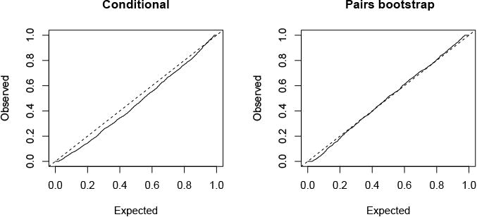
P-values for the lasso in the Gaussian setting: n = 200, p = 50, 20 strong signals. Predictors have pairwise correlation of 0.3 and variance of the errors depends on non-signal variables. Shown are the quantile-quantile plots for the non-signal variables in realizations for which the lasso has successfully screened (captured all of the signal variables). We see that the conditional analysis yields anti-conservative p-values while the pairs bootstrap gives p-values closer to uniform.

4 Simulations

To assess performance in the ℓ₁-penalized logistic model, we generated Gaussian features with pairwise correlation 0.2 in two scenarios: n = 30, p = 10 and n = 40, p = 60. Then y was generated as Pr(Y = 1|x) = 1/(1 + exp(−x^Tβ)). There are two signal settings: null (β = 0) (Figure 3) non-null (β = (5, 0, 0 …)) (Figure 4). Finally, in each case we tried two methods for choosing the regularization parameter λ: a fixed value yielding a moderately sparse model and cross-validation. The figures show the cumulative distribution function of the resulting p-values over 1000 simulations. Thus a function above the 45 degree line indicates an anti-conservative test in the null setting and a test with some power in the non-null case. We see the adjusted p-values are close to uniform under the null in every case and show power in the non-null setting. Even with a cross-validation-based choice for λ the type I error seems to be controlled, although we have no theoretical support for this finding. In Figure 3 we also plot the naive p-values from GLM theory: as expected they are very anti-conservative.

Figure 3.

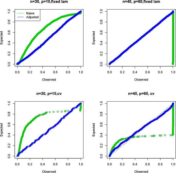
P-values for the logistic regression model, null setting. The top panels use a fixed λ while the bottom ones use cross-validation to choose λ.

Figure 4.

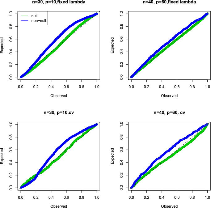
P-values for the logistic regression model, non-null setting. The top panels use a fixed λ while the bottom ones use cross-validation to choose λ.

Figure 5 shows the results of an analogous experiment for the Cox model in the null setting, using exponential survival times and random 50% censoring. Type I error control is good, except in the cross-validation case where it is badly anti-conservative for smaller p-values. We have seen similar behaviour in the Gaussian lasso setting, and this phenomenon deserves further study.

Figure 5.

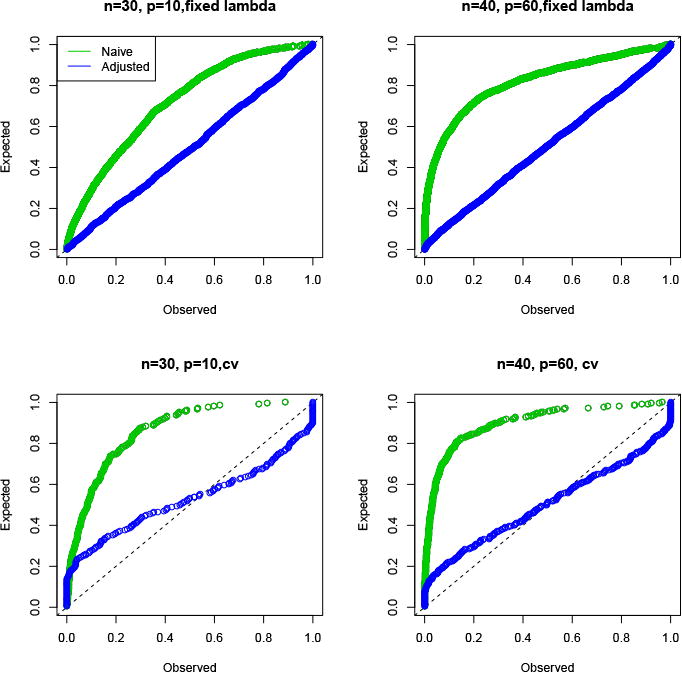
P-values for the Cox Model, null setting. The top panels use a fixed λ while the bottom ones use cross-validation to choose λ.

Table 1 shows the miscoverage and median lengths of intervals for the logistic regression example in the null setting, with a target miscoverage of 10%. The intervals can sometimes be very long, and in fact, have infinite expected length.

Table 1.

Lasso-penalized logistic regression. Details as in Figure 4. Shown are the the miscoverage and median length of selection (confidence) intervals for main proposal of this paper. The target miscoverage is 10%. Selection of λ is done using either a fixed value yielding moderate sparsity or cross-validation (cv).

	N>p, fixed λ	N>p, cv	N<p, fixed λ	N<p, cv
miscoverage	0.11	0.11	0.14	0.14
median length	8.07	6.63	5.75	29.69

As a comparison, Table 2 shows analogous results for Gaussian regression, using the proposal of Lee et al. (2013). For estimation of the error variance σ², we used the mean residual error for N > p and the cross-validation estimate of Reid et al. (2013) for N < p.

Table 2.

Lasso-penalized Gaussian regression. Shown are the miscoverage and median lengths of selection (confidence) intervals based on the Gaussian model of Lee et al. (2013). The target level is 10%. Selection of λ is done using either a fixed value yielding moderate sparsity or cross-validation (cv).

	N > p, fixed λ	N >p, cv	N < p, fixed λ	N < p, cv
miscoverage	0.11	0.12	0.13	0.10
median length	12.29	6.90	20.50	32.06

Again, the intervals can be quite long. There are potentially better ways to construct the intervals: Tibshirani et al. (2015) propose a bootstrap method for post-selection inference that in our current problem would draw bootstrap samples from z₁, z₂, … z_n and use their empirical distribution in the polyhedral lemma (in place of the Gaussian distribution). The “randomized response” strategy provides another way to obtain shorter intervals, at the expense of increased computation: see Tian and Taylor (2015).

5 Examples

5.1 Liver data

The data in this example and the following (edited) description were provided by D. Harrington and T. Fleming.

“Primary biliary cirrhosis (PBC) of the liver is a rare but fatal chronic liver disease of unknown cause, with a prevalence of about 50-cases-per-million population. The primary pathologic event appears to be the destruction of interlobular bile ducts, which may be mediated by immunologic mechanisms.

The following briefly describes data collected for the Mayo Clinic trial in PBC of the liver conducted between January, 1974 and May, 1984 comparing the drug D-penicillamine (DPCA) with a placebo. The first 312 cases participated in the randomized trial of D-penicillamine versus placebo, and contain largely complete data. An additional 112 cases did not participate in the clinical trial, but consented to have basic measurements recorded and to be followed for survival. Six of those cases were lost to follow-up shortly after diagnosis, so there are data here on an additional 106 cases as well as the 312 randomized participants.”

We discarded observations with missing values, leaving 276 observations. The predictors are

• X₁ : Treatment Code, 1 = D-penicillamine, 2 = placebo.

• X₂ : Age in years. For the first 312 cases, age was calculated by dividing the number of days between birth and study registration by 365.

• X₃ : Sex, 0 = male, 1 = female.

• X₄ : Presence of ascites, 0 = no, 1 = yes.

• X₅ : Presence of hepatomegaly, 0 = no, 1 = yes.

• X₆ : Presence of spiders, 0 = no, 1 = yes.

• X₇ : Presence of edema, 0 = no, .5 yes but responded to diuretic treatment, 1 = yes, did not respond to treatment.

• X₈ : Serum bilirubin, in mg/dl.

• X₉ : Serum cholesterol, in mg/dl.

• X₁₀ : Albumin, in gm/dl.

• X₁₁ : Urine copper, in μg/day.

• X₁₂ : Alkaline phosphatase, in U/litre.

• X₁₃ : SGOT, in U/ml.

• X₁₄ : Triglycerides, in mg/dl.

• X₁₅ : Platelet count; coded value is number of platelets per cubic ml. of blood divided by 1000.

• X₁₆ : Prothrombine time, in seconds.

• X₁₇ : Histologic stage of disease, graded 1, 2, 3, or 4.

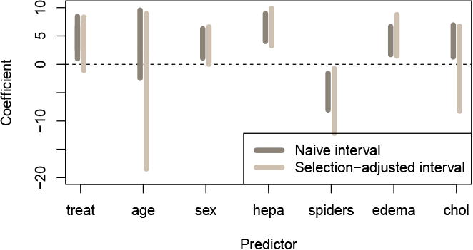
We applied Cox's proportional hazards model. Figures 6 and 7 show the results. As expected, the adjusted p-values are larger than the naive ones and the corresponding selection (confidence) intervals tend to be wider.

Figure 6. P-values for Cox model applied to the liver data.

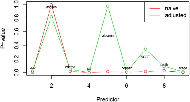
Figure 7. Selection intervals for Cox model applied to the liver data.

6 The Graphical lasso

Another, different, example is the graphical lasso for estimation of sparse inverse covariance graphs. Here we have data X_n×p ∼ N(0, Σ). Let S = X^T X/N, Θ = Σ⁻¹.

We maximize

$$\ell (\mathrm{\Theta })=logdet\mathrm{\Theta }-\text{tr}S\sum -\lambda {\Vert \mathrm{\Theta }\Vert }_1$$ (28)

where the norm in the second is the sum of the absolute values.

The KKT conditions have the form

$${\mathrm{\Theta }}^{-1}-S-\lambda s(\mathrm{\Theta })=0$$ (29)

or for one row/column, Σ₁₁β − s₁₂ − λs(β) = 0, where β is a p − 1 vector in the pth row/column of Θ, excluding the diagonal, and Σ ₁₁ is the block Σ of excluding one row and column. Defining R = d²ℓ/dΘdΘ^T we have

$${\overline{\mathrm{\Theta }}}_M={\widehat{\mathrm{\Theta }}}_M+\lambda R^{-1}{s}_M.$$ (30)

Hence we apply the polyhedral lemma to ${\overline{\mathrm{\Theta }}}_M~N({\mathrm{\Theta }}_M^{\ast },R^{-1})$ with constraints −diag (s_M)(Θ̄_M−R⁻¹ s_M) ≤ 0. From this we can obtain p-values for testing whether a link parameter is zero (H₀ : θ_jk = 0) and confidence intervals for θ_jk. We note the related work on high-dimensional inverse covariance estimation in Jankova and van de Geer (2014).

Figure 8 shows the results of a simulation study with n = 80, p = 20 with the components X₁, X₂, … X_p being standard Gaussian variables. All components were generated independently except for the first two, which had correlation 0.7. A fixed moderate value of the regularization parameter was used. Conditioning on realizations for which the partial correlation for the first two variables was non-zero, the Figure shows the p-values for non-null (1,2) entry and the null (the rest). We see that the null p-values are close to uniform and the non-null ones are (slightly) sub-uniform.

Figure 8.

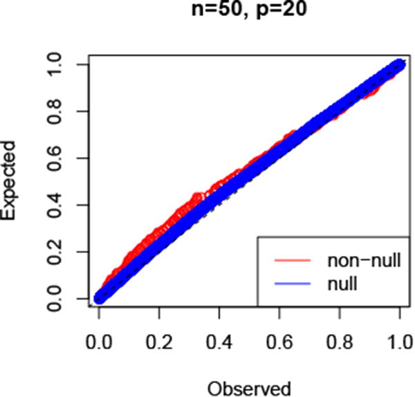
Simulation results: P-values for the graphical lasso. Details are given in the text.

6.1 Example

Here we analyze the protein data discussed in Friedman et al. (2008). The measurements are from flow cytometry, with 11 proteins measured over 7466 cells. Table 3 and Figure 9 show the results of applying the post-selection procedure with a moderate value of the regularization parameter λ. Six interactions are present in the selected model, with only one (Mek-P38) being strongly significant.

Table 3. P-values from the graphical lasso applied to the protein data.

Protein pair	P-values
Raf -Mek	0.789
Mek -P38	0.005
Plcg- PIP2	0.107
PIP2 -P38	0.070
PKA -P38	0.951
P38 -Jnk	0.557

Figure 9.

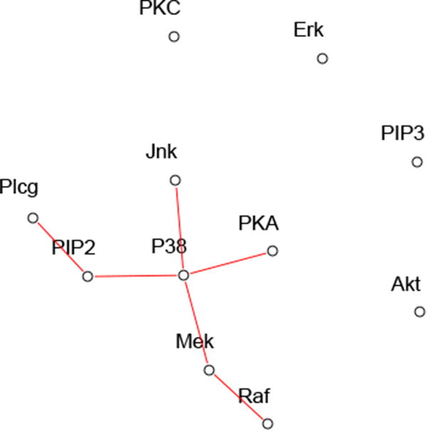
Results for protein data. The red lines indicate non-zero fitted entries in Θ̂.

7 Discussion

We have proposed a method for post-selection inference, with applications to ℓ₁-penalized likelihood models. These include generalized linear models, Cox's proportional hazards model, and the graphical lasso. As noted earlier, while our focus has been on selection via ℓ₁-penalization, a similar approach can be applied to forward stepwise methods for likelihood models, and in principle, least angle regression.

A major challenge remains in the estimation of the tuning parameter λ One possibility is to use a choice proposed by Negahban et al. (2012) (Theorem 1), which is λ′ = 2⋅E[max_j ∇ L(0)]. In the logistic and Cox models, for example, this is not a function of y and hence the proposals of this paper can be applied. More generally, it would be desirable to allow for the choice of λ by cross-validation in our methodology. Choosing λ by cross-validation is feasible, particularly in the “randomized response” setting of Tian and Taylor (2015) though this approach requires MCMC for inference. A related approach to selective inference after cross-validation is described in Loftus (2015).

The proposals of this paper are implemented in our selectiveInference R package in the public CRAN repository.

Appendix

The Polyhedral lemma and truncation limits for post-selection Gaussian inference

Let y ∼N(μ, Σ) and suppose that we apply the lasso with parameter λ to data (X, y), yielding active variables M. Lee et al. (2013) show that for the active variables, $A_1=-D{(X_M^T{X}_M)}^{-1}{X}_M^T,b_1=-D{(X_M^T{X}_M)}^{-1}\lambda s$ where D = diag(s). For inactive variables, $A_0=\frac{1}{\lambda }\left(\begin{array}{c}{X}_{-M}^T\\ -X_{-M}^T\end{array}\right),b_0=\left(\begin{array}{c}1+X_{-M}^T{X}_M\widehat{\beta }/\lambda \\ 1-X_{-M}^T{X}_M\widehat{\beta }/\lambda \end{array}\right)$

Finally, we define $A=\left(\begin{array}{c}{A}_1\\ A_0\end{array}\right)$, b = (b₁, b₀). They also show that

$$\{Ay\le b\}=\{{\nu }^{-}(y)\le {\gamma }^{T}y\le {\nu }^{+}(y),{\nu }^0(y)\ge 0\},$$ (31)

and furthermore, γ^T y and (ν⁻(y), ν⁺(y), ν⁰(y)) are statistically independent. This surprising result is known as the polyhedral lemma. Let c ≡ Σ_γ(γ^TΣ_γ)⁻¹, and r ≡ (I_N − c_γ^T)y. Then the three values on the righthand side of (31) are computed via

$$\begin{array}{ccc}{\nu }^{-1}(r)& =& \underset{j:{(Ac)}_j<0}{max}\frac{b_j-{(Ar)}_j}{{(Ac)}_j}\\ {\nu }^{+1}(r)& =& \underset{j:{(Ac)}_j>0}{min}\frac{b_j-{(Ar)}_j}{{(Ac)}_j}\\ {\nu }^0(r)& =& \underset{j:{(Ac)}_j=0}{min}{b}_j-{(Ar)}_j.\end{array}$$ (32)

Hence the selection event {Ay ≤ b} is equivalent to the event that γ^T y falls into a certain range, a range depending on A and b. This equivalence and the independence means that the conditional inference on γ^T μ can be made using the truncated distribution of γ^T y, a truncated normal distribution.

The Hessian for the graphical lasso

Let (Δ_ij)_{1≤i≤j≤p} denote the upper triangular parameters for the graphical lasso and

$$\mathrm{\Theta }{(\mathrm{\Delta })}_{ij}=\{\begin{array}{cc}{\mathrm{\Delta }}_{ji}& i>j\\ {\mathrm{\Delta }}_{ij}& i\le j\end{array}$$

be the symmetric version so that

$$\frac{\partial }{\partial {\mathrm{\Delta }}_{ij}}{\mathrm{\Theta }}_{kl}={\delta }_{ik}{\delta }_{jl}+{\delta }_{il}{\delta }_{jk}.$$

Now,

$$\frac{{\partial }^2}{\partial {\mathrm{\Theta }}_{ij}\partial {\mathrm{\Theta }}_{kl}}(-logdet\mathrm{\Theta })=\text{Tr}(e_i{e}_j^T{\mathrm{\Theta }}^{-1}{e}_k{e}_l^T{\mathrm{\Theta }}^{-1})={\sum }_{jk}{\sum }_{il}$$

with Σ = Θ⁻¹. Note that we evaluate this at a symmetric matrix, i.e. Θ^T = Θ.

Therefore,

$$\begin{gathered} \frac{{\partial }^2}{\partial {\mathrm{\Delta }}_{ij}\partial {\mathrm{\Delta }}_{kl}}(-logdet(\mathrm{\Theta }(\mathrm{\Delta }))) \\ =\sum _{i^{\prime },j^{\prime },k^{\prime },l^{\prime }}{\sum }_{j^{\prime }{k}^{\prime }}{\sum }_{i^{\prime }{l}^{\prime }}({\delta }_{i{i}^{\prime }}{\delta }_{j{j}^{\prime }}+{\delta }_{i{j}^{\prime }}{\delta }_{j{i}^{\prime }})({\delta }_{k{k}^{\prime }}{\delta }_{l{l}^{\prime }}+{\delta }_{k{l}^{\prime }}{\delta }_{l{k}^{\prime }}) \\ =2({\sum }_{il}{\sum }_{jk}+{\sum }_{ik}{\sum }_{jl}). \end{gathered}$$

References

- Bickel PJ, Klaassen CA, Ritov Y, Wellner JA. Efficient and adaptive estimation for semiparametric models. Johns Hopkins Univ. Press; Baltimore: 1993. [Google Scholar]
- Bühlmann P. Statistical significance in high-dimensional linear models. Bernoulli. 2013;19(4):1212–1242. [Google Scholar]
- Buja A, Berk R, Brown L, George E, Pitkin E, Traskin M, Zhang K, Zhao L. A Conspiracy of Random X and Nonlinearity against Classical Inference in Linear Regression. 2016 submitted. [Google Scholar]
- Bunea F. Honest variable selection in linear and logistic regression models via l1 and l1+enalization. Electron J Statist. 2008;2:1153–1194. doi: 10.1214/08-EJS287. URL: [DOI] [Google Scholar]
- Fithian W, Sun D, Taylor J. Optimal inference after model selection. ArXiv e-prints 2014 [Google Scholar]
- Friedman J, Hastie T, Tibshirani R. Sparse inverse covariance estimation with the graphical Lasso. Biostatistics. 2008;9:432–441. doi: 10.1093/biostatistics/kxm045. [DOI] [PMC free article] [PubMed] [Google Scholar]
- Hastie T, Tibshirani R. Generalized Additive Models. Chapman & Hall; London: 1990. [DOI] [PubMed] [Google Scholar]
- Jankova J, van de Geer S. Confidence intervals for high-dimensional inverse covariance estimation. 2014 arXiv:1403.6752. [Google Scholar]
- Javanmard A, Montanari A. Confidence intervals and hypothesis testing for high-dimensional regression. Journal of Machine Learning Research. 2014;15:2869–2909. [Google Scholar]
- Lee J, Sun D, Sun Y, Taylor J. Exact post-selection inference, with application to the Lasso. 2013 arXiv:1311.6238. [Google Scholar]
- Loftus JR. Selective inference after cross-validation. ArXiv e-prints 2015 [Google Scholar]
- Negahban SN, Ravikumar P, Wainwright MJ, Yu B. A unified framework for high-dimensional analysis of m-estimators with decomposable regularizers. Statist Sci. 2012;27(4):538–557. doi: 10.1214/12-STS400. URL: [DOI] [Google Scholar]
- Reid S, Tibshirani R, Friedman J. A Study of Error Variance Estimation in Lasso Regression. 2013 ArXiv e-prints to appear Statistica Sinica. [Google Scholar]
- Taylor J, Lockhart R, Tibshirani2 R, Tibshirani R. Post-selection adaptive inference for least angle regression and the Lasso. 2014 arXiv:1401.3889; submitted. [Google Scholar]
- Taylor J, Tibshirani RJ. Statistical learning and selective inference. Proceedings of the National Academy of Sciences. 2015;112(25):7629–7634. doi: 10.1073/pnas.1507583112. URL: http://www.pnas.org/content/112/25/7629.abstract. [DOI] [PMC free article] [PubMed] [Google Scholar]
- Tian X, Taylor JE. Asymptotics of selective inference. ArXiv e-prints 2014 [Google Scholar]
- Tian X, Taylor JE. Selective inference with a randomized response. ArXiv e-prints 2015 [Google Scholar]
- Tibshirani RJ, Rinaldo A, Tibshirani R, Wasserman L. Uniform Asymptotic Inference and the Bootstrap After Model Selection. ArXiv e-prints 2015 [Google Scholar]
- Tibshirani2 R. The Lasso problem and uniqueness. Electronic Journal of Statistics. 2013;7:1456–1490. [Google Scholar]
- Tropp J. Greed is good: algorithmic results for sparse approximation. Information Theory, IEEE Transactions on. 2004;50(10):2231–2242. [Google Scholar]
- van de Geer S, Bühlmann P, Ritov Y, Dezeure R. On asymptotically optimal confidence regions and tests for high-dimensional models. 2013 arXiv:1303.0518v2. [Google Scholar]
- Wainwright M. Sharp thresholds for high-dimensional and noisy sparsity recovery using l1-constrained quadratic programming (lasso) Information Theory, IEEE Transactions on. 2009;55(5):2183–2202. [Google Scholar]
- Zhang CH, Zhang S. Confidence intervals for low-dimensional parameters with high-dimensional data. Journal of the Royal Statistical Society Series B. 2014;76(1):217–242. [Google Scholar]