Future population and human capital in heterogeneous India

Significance

India will soon be the world’s most populous country, but in terms of human capital and, consequently, Gross Domestic Product per capita, it has been trailing behind China. While some economists believe that India’s younger population will be an advantage over China’s aging one, here we show that much will depend on future investments in education and health and thus human capital. In terms of methodology, this paper addresses the question of what sources of observable population heterogeneity should be explicitly incorporated in population projections. It suggests that the dominant model of considering only the age and sex structures at the national level should be complemented by multidimensional models depending on the importance of heterogeneity and substantive user interest in the additional dimensions.

Abstract

Within the next decade India is expected to surpass China as the world’s most populous country due to still higher fertility and a younger population. Around 2025 each country will be home to around 1.5 billion people. India is demographically very heterogeneous with some rural illiterate populations still having more than four children on average while educated urban women have fewer than 1.5 children and with great differences between states. We show that the population outlook greatly depends on the degree to which this heterogeneity is explicitly incorporated into the population projection model used. The conventional projection model, considering only the age and sex structures of the population at the national level, results in a lower projected population than the same model applied at the level of states because over time the high-fertility states gain more weight, thus applying the higher rates to more people. The opposite outcome results from an explicit consideration of education differentials because over time the proportion of more educated women with lower fertility increases, thus leading to lower predicted growth than in the conventional model. To comprehensively address this issue, we develop a five-dimensional model of India’s population by state, rural/urban place of residence, age, sex, and level of education and show the impacts of different degrees of aggregation. We also provide human capital scenarios for all Indian states that suggest that India will rapidly catch up with other more developed countries in Asia if the recent pace of education expansion is maintained.

At the time of independence in 1947, India’s total population was around 370 million and Indian women on average had six children. The age structure was very young, and over 80% of the population was illiterate (1). As a consequence, the population grew very rapidly, raising early concerns about the sufficiency of food supply and development prospects in general. Given these fears, in the late 1960s the Ford Foundation commissioned the “Second India” study to understand how India would fare under an expected doubling of its population (hence the name of the study) (2). In 1965 India’s population was 500 million, and shortly before 2000 it reached the 1 billion mark. Revisiting the Second India around that time, Cassen found a rather mixed record. Some issues such as food production turned out to be better than feared, while others such as lack of education and poverty were worse than hoped (2). Both authors pointed at the great heterogeneity of the subcontinent, illustrated by the fertility rates in the early 1990s, which had already declined to 1.8 children per woman in Kerala but still stood at 5.1 in Uttar Pradesh (3).

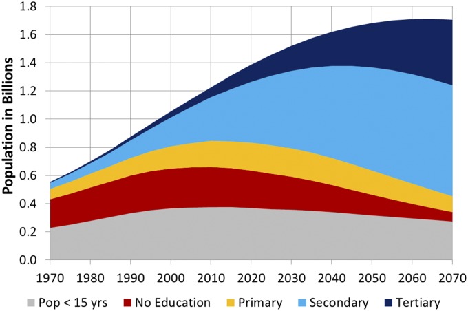
The great heterogeneity of the Indian population is also the main focus of this paper. We will show how different ways of explicitly addressing heterogeneity in our demographic models will produce different outlooks for India’s future population, human capital, and thus development. Fig. 1 shows the evolution of one century of India’s population by level of education as observed since 1970 and forecast under a model described in this paper. It shows that in the 1970s still far more than half of the entire adult population had never received any formal education and that this unfavorable situation has changed only very slowly. Still, by 1990, half of the adult population had never been to school.

Fig. 1.

India’s total population 1970–2070 by level of education (23).

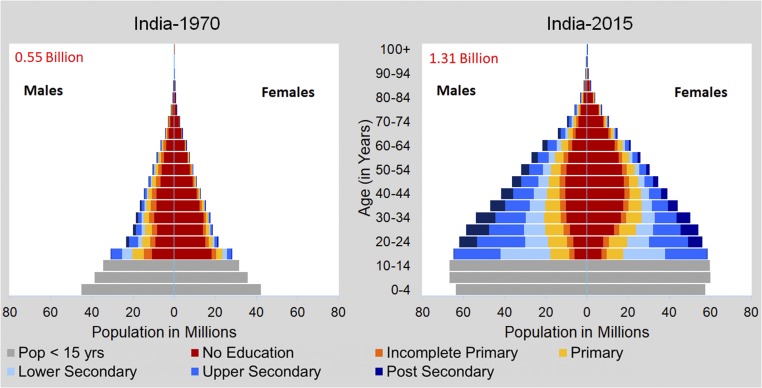
Educational attainment of women has been much worse than that of men. Fig. 2 shows the age and education pyramids for 1970 and 2015. It shows that in 1970 about three quarters of Indian adult women had never been to school. Only a very tiny elite had the privilege of education. Among the younger cohorts, the proportion with at least primary education starts to slowly increase. For males, education levels are remarkably higher with only fewer than half of all adult men never having been to school. Because of higher fertility levels—during the 1960s Indian women had on average almost six children—the population age structure in 1970 was still extremely young. This very young age structure, together with only slow declines in birth rates, resulted in an increase of India’s population from 554 million in 1970 to 1.3 billion in 2015. Today the younger cohorts are significantly better educated, but the legacy of low levels of female education is still visible in the low educational attainment of older cohorts, particularly of women. In association with the improving education of younger women, national-level fertility rates have also declined to 2.2, which is just around a third of their levels in the 1960s.

Fig. 2.

Age and education pyramids for India (national level) for 1970 and 2015 (23).

In this paper we will address the likely future population trends of India while systematically accounting for India’s great population heterogeneity. Earlier projections of India that tried to go beyond conventional aggregate projections by age and sex revealed an interesting phenomenon, namely that projections turn out to be significantly higher or lower depending on what additional sources of heterogeneity are taken into account. One study (4) showed that, if the projection is carried out at the level of India’s 35 states, then the sum of state projections turns out to be significantly higher due to the fact that the high-fertility states over time receive more weight, and thus the higher fertility rates are applied to relatively more women. In contrast, projections that differentiated by level of educational attainment (at the national level) (5) resulted in lower forecasts because over time the younger, more educated cohorts of women entered the main reproductive ages, and since higher education is associated with lower fertility, this led to lower overall fertility.

These seemingly contradictory results, which depend on which source of evident population heterogeneity is included in the model, lead to the more general methodological debate in population forecasting and even more broadly for all social and economic forecasting models. What is the most appropriate way to account for the observable heterogeneity of agents in forecasts? While unobservable population heterogeneity also matters (6), the options to account for it are limited, a fact that suggests caution when interpreting results. Observed population heterogeneity, on the other hand, could readily be incorporated into multidimensional models, but there has been an interesting debate about whether this should always be done, most prominently in a set of papers in 1995 on the question of whether simple models outperform complex ones (7). This discussion focused primarily on the question of whether forecasting total population size directly by applying assumed growth rates has given more accurate projections than the more complex cohort-component methods projecting individual age cohorts. In this context, Long (8) stresses that one needs to distinguish between two different questions: (i) whether one is only interested in the difference it makes for total population size forecasts and (ii) whether the additional dimension considered is of interest in its own right. We will add to this methodological discussion through an ex ante analysis of the sensitivity of Indian population forecasts to different sources of heterogeneity in the context of a multidimensional model, which, in addition to the conventional age and sex structure, also explicitly differentiates by level of educational attainment, urban/rural place of residence, and state of residence with differential fertility and mortality rates.

Heterogeneous India

India is a subcontinent that includes many population groups differing by language, ethnicity, religion, and caste (3). While some of this heterogeneity is stratified spatially and can be captured by differentiating between states and urban and rural areas, other factors (such as caste) exist in almost every location. Since statistical information tends to be collected along administrative boundaries, regional differentiation can be captured more easily from official aggregate statistical sources. Some of the other sources of heterogeneity can be derived only from individual-level data or more detailed cross-tabulations of census data. As has been argued earlier (9) and recently by Lutz and KC (10), the level of educational attainment and urban/rural place of residence are the two most important demographic dimensions of population heterogeneity after age and sex that cover relevant sociodemographic differentiations and should be used when measuring and modeling population dynamics. Following this approach, this study uses data that differentiate the populations of each of the 35 Indian states by all four dimensions (age, sex, level of education, and urban/rural place of residence).

The data used in this study come from detailed tabulations of the two most recent Indian censuses that were conducted in 2001 and 2011. These census tabulations were complemented with respect to vital rates by tabulations from the Sample Registration Survey (SRS) with annual information for the years 1999–2013. This allows us not only to study cross-sectional information, but also to analyze the trends over time since 1999. A more detailed specification of the data sources is given in SI Appendix.

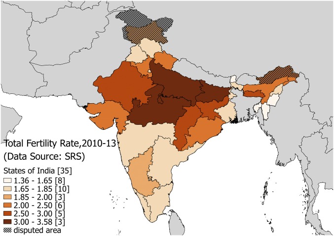
Since fertility levels are the most important source of differential population growth, we studied the regional demographic heterogeneity first through the lens of fertility. The map of India’s 35 states and union territories according to their fertility levels in 2010–2013 (Fig. 3) shows a distinct pattern of North–South differences with some interesting exceptions. Fertility is highest in the big states of the northwestern India—above three children per woman in Bihar, Uttar Pradesh, and Madhya Pradesh, with Rajasthan and Jharkhand being very close to that level. On the other end of the spectrum are eight small states and union territories with fertility levels of less than 1.6. But even the big southern states of Andhra Pradesh, Kerala, and Tamil Nadu are well below 2.0. As will be discussed below, these differences to a large extent can be explained by different levels of social and economic development, but there remain some relevant cultural differences as well. Odisha is an example where, despite a low level in terms of social and economic development, fertility level has been relatively low due to extensive family planning drives in some parts of India (3, 11).

Fig. 3.

Map of Indian states. Color codes for TFR (24).

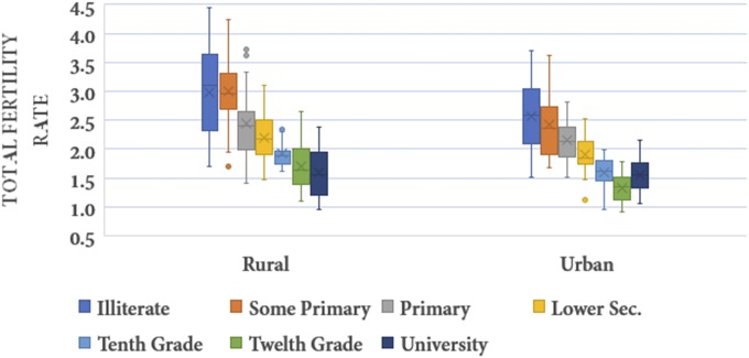
Next, we look at the further stratification of fertility levels by maternal education and urban/rural place of residence (Fig. 4). Here we see a very consistent, almost linear, decline of fertility by levels of education with only a slight reversal for the very highest group. For rural fertility at the national level, total fertility rate (TFR) is 3.2 for illiterate women, declines to 2.6 for those with completed primary education, and bottoms at 1.7 for those with completed secondary education. For urban women, the slope of the gradient is about the same, but the level of the line is about half a child lower, starting at 2.6 for illiterate women to 1.3 for women with completed secondary education. While the line gives the national average, there clearly is some variation around these averages at the state level. The variation can be explained in terms of social, economic, and cultural differences as well as varying levels of success in family-planning drives among the poor and less educated population at the state level (3, 11). In addition, the education distribution within each education category could also be a reason for the variation.

Fig. 4.

Total fertility rates in India by place of residence and education of the mother, distributions across states and territories (box shows 50% range, lines span full range, and points are outliers) (24).

Illustrative Constant Rates Scenario

For analytically comparing the effect of different forms of aggregation on project results, one must compare projections with equivalent fertility, mortality, migration, and education assumptions. This raises problems for any kind of more realistic projection that assumes continued changes of these rates in the future because the assumptions about these changes must be made for some specific level of aggregation. If we want to make “identical” assumptions at different levels of aggregation, then the easiest way of doing so is to simply hold constant all of the currently observed rates at all levels of aggregation. This freezing of transition rates at their current level will result in differences that can be entirely attributed to the effects of different levels of aggregation. The resulting differences will be the consequence of projection “errors” that result from assuming population homogeneity where actually there is measurable heterogeneity. The result will also allow us to understand which sources of heterogeneity, of the ones considered here, are more relevant in influencing results. The findings of this systematic comparison have important general implications for the way in which population projections should be done in the future.

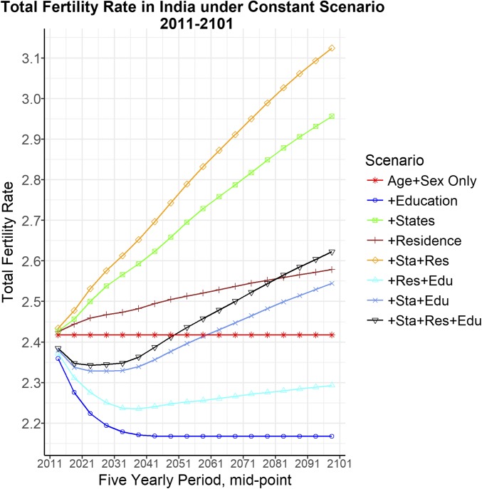
Fig. 5 shows the aggregate national TFR for India, resulting from assuming constant fertility rates at different levels of aggregation. Starting from the baseline TFR of slightly above 2.4, the straight red horizontal line gives the national level TFR, which is invariant when it is assumed to be constant at the national level without considering heterogeneity. If fertility rates are held constant at the level of the 35 states and union territories of India, then TFR will increase almost linearly to close to 3.0 by the end of the century because over time the high fertility states will see higher population growth and thus their higher fertility level will gradually carry more weight in determining the national fertility level. However, when fertility rates are kept constant at the level of the six different education groups without considering the state of residence, then the national-level fertility declines sharply over the coming two decades before leveling off. This is due to the education momentum that is already embedded in the population structure with the young cohorts of women being significantly better educated than the average woman in reproductive age today. These better-educated young cohorts will gradually move up the age pyramid and hence lower the average fertility of reproductive-age women. But this effect will be happening only over the next two decades because in this scenario school enrollment rates are also kept constant and the new cohorts entering school age will not see any further improvements in education, which translates into no further decline in fertility under this constant scenario.

Fig. 5.

National-level TFR in India under constant scenario at different levels of disaggregation.

These results show numerically the above-described issue, which in part motivated this study. The two projections accounting for different sources of heterogeneity (one by states, the other by education) yielded deviations from the aggregate-level projection that go in different directions. Fig. 5 also shows that disaggregation by urban/rural place of residence goes in the same direction as states, and thus considering both together, yields the highest aggregate fertility. When combining education and urban/rural place of residence that have effects in opposing directions, then the education effect clearly dominates. The most interesting case is to see what happens when state, place of residence, and education effects (two working upward and one working downward) are combined. Here, first the education effect dominates and leads to lower fertility until around 2050, after which point the state and place of residence effects dominate.

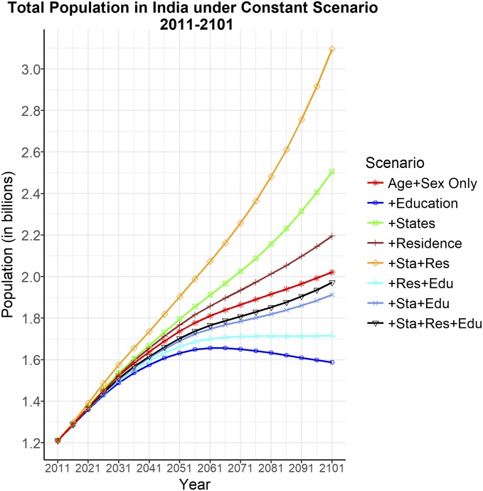
Fig. 6 shows the results of these different fertility levels together with all other demographic rates held constant at the indicated levels. The resulting population sizes by the end of the century span a huge range from 1.6 billion in the case of stratifying only by level of education to 3.1 billion in the case of stratifying only by state and place of residence. Considering that these results (differing by 1.5 billion people) come from identical assumptions that keep all demographic rates constant and vary only the source of heterogeneity explicitly included in the model suggests the critical importance of the question of which heterogeneity to include in the model (discussed further in the concluding section).

Fig. 6.

Resulting total population sizes for India under constant scenario at different levels of disaggregation.

A Multidimensional Medium Scenario for India

To come up with a realistic population scenario that incorporates what is seen from today’s perspective as the most likely future trajectories of fertility, mortality, migration, and education, we conducted a very detailed analysis of education-specific trends in 70 territorial units of India (urban and rural for each of the 35 states and union territories). Since full documentation of these specific analyses is given elsewhere (12), here we summarize only the basic findings and choices that went into defining the medium scenario. To make the study comparable across demographic components, similar methods were used to define the models generating the assumptions for all 70 territorial units. Hence, we developed a fertility model, a mortality model, a migration model, and an education model that will be briefly outlined in the following sections.

Fertility.

In terms of the fertility model, a method was developed to extend into the future the empirically given trends of age- and education-specific fertility rates (by state and urban/rural) from the period 1999–2013. General trends show that fertility has been declining rapidly among women with no education or some primary education, while rates among women with completed primary and lower secondary education declined more slowly with a tendency to level off. Fertility among women with the highest education seems to have largely leveled off at rates well below replacement fertility. Since these trends showed slightly different patterns for urban and rural women, two separate models were developed. Both models are based on fitting a spline through the data points that aligns the trends over time for each education group with the cross-sectional pattern of lower fertility by level of education, which tends to show a rather clear general trend from high to low fertility levels. Since, for the highest education group (university), both the cross-sectional pattern as well as the trend over time show a minor increase after reaching very low levels (a TFR of 1.73 for rural and 1.40 for urban, which are floor values), this light upswing is also reflected in the fertility model that will eventually converge to a level of 2.08 in urban and 1.75 in rural areas (see SI Appendix for details). This is also in line with what the United Nations (UN) assumes for long-term fertility assumptions of low-fertility countries (UN 2017 assessment) and can also be explained in terms of a to-be-expected end of the tempo effect that depresses period fertility due to postponement of childbearing (13). At the national level these assumptions imply that fertility across all education groups would reach a bottom of around 1.4 in 60 y for urban areas and of around 1.73 in 80 y for rural areas. With different starting values, all states will follow the rural- and urban-specific trajectories into the future (see SI Appendix for details).

Mortality.

As for mortality, sex-specific life tables of each state were taken separately for rural and urban areas from the SRS website (14). These life tables were estimated based on registered deaths during 2009–2013. Unfortunately, no education-specific life tables were available, not even at the national level. The only source of information for differential mortality is child mortality by mother’s education as recorded in demographic surveys. Therefore, using the Indian Demographic and Health Survey (15), we calculated differential mortality by mother’s education and used this to estimate adult mortality differentials using model life tables. While this may result in a slight overestimation of mortality differentials if child mortality is more sensitive to education than adult mortality, it is still preferable to disregarding educational differentials, which implicitly assumes a certainly incorrect zero difference.

The SRS estimates for life expectancy at birth at the national level were 69.3 y for women and 65.8 y for men for the period around 2011. This sex difference in mortality in India is somewhat lower than in most other countries, and only since the 1980s has the original pattern of higher female mortality been reversed. Before then, India was one of the few countries where men lived longer than women, presumably due to differential treatment. In the coming decades we assume India will move toward the standard international sex differentials in mortality.

For projecting life expectancy into the future, we generated an average pathway for future gain by regressing gains in life expectancy between two observed points in time using time-series data for several periods spanning 1970–2013 (SRS) separately for males and females. This takes into account the fact that at high levels of life expectancy potential gains tend to diminish. We fit a simple linear regression and extrapolated life expectancy into the future using the regression results to generate the general predicted average gain. For men and women in each territory, we started with the recently observed average rate of change and then let it converge to the general predicted average gain by 2030. On average, this gain starts out to be somewhat above 2 y per decade and carries on until the end of the century at somewhat below 2 y per decade.

Migration.

Internal migration between rural and urban regions within and between the states is one of the main determinants of regional population dynamics in India. The data for bilateral flows between all of the rural and urban areas in all states were not readily available and had to be estimated from different tables from the Census 2001 as the relevant data from the 2011 census has not yet published. A detailed account of this estimation procedure and its results is given in SI Appendix.

Education.

This study distinguishes between six levels of educational attainment ranging from illiterate to university. The given educational attainment distributions for women and men in 2011 in each of the 70 urban and rural territories was used to reconstruct the distributions in earlier years by going back along cohort lines. This utilizes the fact that educational attainment is typically acquired at a younger age and then stays invariant over the rest of life. Hence, if we know how many 60-y-old women are high school graduates, we also know how many 30 y olds were high school graduates 30 y ago. From this information, detailed analysis of trends in educational attainment progression rates by sex were produced for all urban and rural areas. The Indian Education Trend scenario then assumes that these trends will continue in the future, where only for tertiary education a ceiling of 50% for rural and 70% for urban men and women is assumed. Since recent progress in education in India has been very impressive, the continuation will result in further rapid education expansion. As a contrast, below we will also discuss the Constant Enrollment Rates Scenario, which shows the implications of the hypothetical case of no further education expansion.

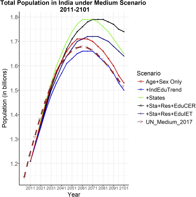
A comparison of the different scenarios based on medium-level assumptions for all of the components confirms the differences between the models including alternative sources of heterogeneity that had been identified for the constant scenario above. But the differences in population size turn out to be smaller than under the constant rates scenario due to smaller differences in future fertility and mortality levels resulting from assumptions of convergence. Over the next two to three decades the results hardly differ because of the common effect of population momentum and the only gradually increasing differences in rates, all hitting the 1.6 billion mark between 2036 and 2046 (Fig. 7). However, in terms of births the differences in the trajectories start earlier with 2.3% in 2011–2016 between the age-and-sex-only model and the age-sex-education model, increasing to around 7% for the next 25 y.

Fig. 7.

Resulting population size of India as a consequence of applying the medium scenario assumptions to models accounting for different sources of heterogeneity. CER, Constant Enrollment Rate; IET, Indian Education Trend.

After 2040 the paths in total population size diverge, with India’s population peaking at quite different levels and at different points in time. The red line in Fig. 7 gives the conventional national-level projection in which only the age and sex structures are considered. Here the population will peak at 1.71 billion in 2056–2066 and then enter a slow decline. Fig. 7 also gives the medium variant of the UN projections for India (thick broken line), which is based on an age- and sex-only model but assumes slightly lower fertility than our age- and sex-only model. This is why it results in somewhat lower projections that after 2070 are almost identical with our Indian education trend scenario. This also reminds us of the fact that the heterogeneity effect discussed in this paper is only one dimension of uncertainty while different assumptions on future fertility levels may even have bigger impacts on the outcomes.

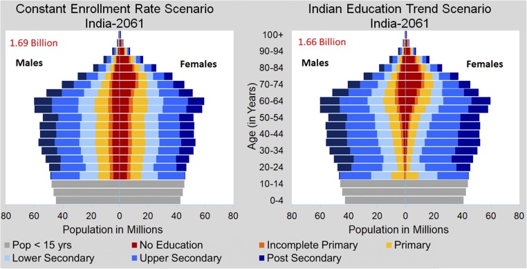
As expected, the lowest projection comes from the model that considers only age, sex, and level of education, showing that the population will peak at 1.66 billion. If only the states are being considered and education is disregarded, the results peak at almost 1.8. The full model—considering all five dimensions—first (dark blue line) produces a lower trajectory than the conventional age-and-sex-only model (red line) due to a dominating education effect, but at 2061 the two lines cross and it climbs higher due to the state effect dominating. Finally, Fig. 7 also shows the line for the full scenario in which medium fertility, mortality, and migration assumptions are combined with the assumption of constant school enrollment rates. Because of the great momentum of changes in the educational composition by cohort, this results in the highest population growth only toward the end of the century. But, as Fig. 8 clearly shows, the two different education scenarios show quite different education distributions for the younger age groups in 2061. Since the Indian education expansion has not yet reached all parts of the population, cessation of further expansions would result in a sizable segment of the population with very low or no education.

Fig. 8.

Education and age pyramids for India as projected to 2061 by the medium scenario combined with the education trend scenario (Left) and the Constant Enrollment Rate Scenario (Right).

Outlook and Conclusions

This study has provided insights with implications for the future of India as well as for the future of producing population projections around the world. We have shown how different degrees of accounting for measurable heterogeneity within populations changes the way in which we see the future. No universally valid recommendation can be derived, and we suggest following Long’s (8) pragmatic suggestion to include those dimensions that are informative for the users and for which an empirical basis exists. While age and sex are explicitly included by most producers of population forecasts, we have concluded that education should also be routinely included because it has well-established implications for fertility and mortality (10, 16), all methods and data are readily available, and the future educational attainment distributions are of great interest in their own right as indicators of a country’s future human capital and development potential (17, 18).

Since independence, India has seen tremendous expansion in its population size, which has increased by a factor of 3.6 up to today. In the past, only elites were educated, with the majority of the population and in particular women never receiving any schooling. Still, in 1990, 70% of adult women had never attended any school, a proportion that subsequently has declined to 46% today. In parallel, the proportion of adult women with some tertiary education increased from 3 to 7%. Hence, recent years have seen a rapid improvement in education, and a look at younger cohorts shows that India is set for further rapid expansion. Among women aged 15–19 today, only 14% are without formal schooling, and already 65% have completed junior secondary or higher levels. Given the consistent evidence of the importance of broad-based education, benefits ranging from poverty eradication and economic growth to health and well-being to quality of institutions and even democracy (18–22) suggest likely future improvements in human development. But our analysis also shows that, if the education expansion should stall in the near future, some of this potential benefit might be lost.

Where does this leave us with respect to comparison of the world’s two billion-plus populations? Because China has massively invested in universal education since the 1950s, it is about three to four decades ahead of India in terms of human capital. Actually, the education pyramid of India today looks similar to that of China around 1980. And the one projection given here for India in 2050 looks similar to that of China today. While cultural and institutional factors may differ between the two countries, and there can be no perfect analogy, this comparison makes it look likely that India will experience similarly rapid human-capital–driven development as China has over the past three to four decades.

References

- 1.National Informatics Centre 2007 Economic Survey 2006-2007: 9.4 State-wise literacy rates (1951-2001) (National Informatics Centre, Ministry of Finance, New Delhi). Available at https://www.indiabudget.gov.in/es2006-07/chapt2007/tab94.pdf. Accessed December 7, 2017.
- 2.Cassen R. Review of the “Second India” revisited: Population, poverty, and environmental stress over two decades. Popul Dev Rev. 1995;21:163–170. [Google Scholar]
- 3.James KS. India’s demographic change: Opportunities and challenges. Science. 2011;333:576–580. doi: 10.1126/science.1207969. [DOI] [PubMed] [Google Scholar]
- 4.Haub C, Sharma OP. India’s Population Reality: Reconciling Change and Tradition. Population Reference Bureau; Washington, DC: 2006. [Google Scholar]
- 5.Lutz W, Scherbov S. Probabilistic population projections for India with explicit consideration of the education-fertility link. Int Stat Rev. 2004;72:81–92. [Google Scholar]
- 6.Vaupel JW, Yashin AI. Heterogeneity’s ruses: Some surprising effects of selection on population dynamics. Am Stat. 1985;39:176–185. [PubMed] [Google Scholar]
- 7.Rogers A. Population forecasting: Do simple models outperform complex models? Math Popul Stud. 1995;5:187–202, 291. doi: 10.1080/08898489509525401. [DOI] [PubMed] [Google Scholar]
- 8.Long JF. Complexity, accuracy, and utility of official population projections. Math Popul Stud. 1995;5:203–216. [Google Scholar]
- 9.Lutz W, Goujon A, Doblhammer-Reiter G. Demographic dimensions in forecasting: Adding education to age and sex. Popul Dev Rev. 1998;24:42–58. [Google Scholar]
- 10.Lutz W, KC S. Dimensions of global population projections: What do we know about future population trends and structures? Philos Trans R Soc Lond B Biol Sci. 2010;365:2779–2791. doi: 10.1098/rstb.2010.0133. [DOI] [PMC free article] [PubMed] [Google Scholar]
- 11.Bhat PM. Returning a favor: Reciprocity between female education and fertility in India. World Dev. 2002;30:1791–1803. [Google Scholar]
- 12.KC S, Speringer M, Wurzer M. 2017 doi: 10.1073/pnas.1722359115. Population projection by age, sex, and educational attainment in rural and urban regions of 35 provinces of India, 2011-2101: Technical report on projecting the regionally explicit socioeconomic heterogeneity in India (International Institute for Applied Systems Analysis, Laxenburg, Austria). Available at pure.iiasa.ac.at/id/eprint/14516/1/WP-17-004.pdf. [DOI] [PMC free article] [PubMed]
- 13.Sobotka T, Lutz W. Misleading policy messages derived from the period TFR: Should we stop using it? Comp Popul Stud-Z Für Bevölkerungswissenschaft. 2011;35:637–664. [Google Scholar]
- 14.ORGI 2014 Sample registration system statistical report 2013 (Office of Registrar General of India, New Delhi). Available at www.censusindia.gov.in/vital_statistics/SRS_Reports_2013.html. Accessed February 10, 2017.
- 15.USAID 2006 Demographic and health survey India 2005/2006 (ICF International, Rockville, MD). Available at www.dhsprogram.com/Data/. Accessed June 4, 2016.
- 16.Lutz W, Butz WP, KC S. World Population and Human Capital in the Twenty-First Century. Oxford Univ Press; Oxford: 2014. [Google Scholar]
- 17.Lutz W. Global sustainable development priorities 500 y after Luther: Sola schola et sanitate. Proc Natl Acad Sci USA. 2017;114:6904–6913. doi: 10.1073/pnas.1702609114. [DOI] [PMC free article] [PubMed] [Google Scholar]
- 18.Lutz W, Cuaresma JC, Sanderson W. Economics. The demography of educational attainment and economic growth. Science. 2008;319:1047–1048. doi: 10.1126/science.1151753. [DOI] [PubMed] [Google Scholar]
- 19.Lutz W, Cuaresma JC, Abbasi-Shavazi MJ. Demography, education, and democracy: Global trends and the case of Iran. Popul Dev Rev. 2010;36:253–281. doi: 10.1111/j.1728-4457.2010.00329.x. [DOI] [PubMed] [Google Scholar]
- 20.Lutz W, Muttarak R. Forecasting societies’ adaptive capacities through a demographic metabolism model. Nat Clim Chang. 2017;7:177–184. [Google Scholar]
- 21.Pamuk ER, Fuchs R, Lutz W. Comparing relative effects of education and economic resources on infant mortality in developing countries. Popul Dev Rev. 2011;37:637–664. doi: 10.1111/j.1728-4457.2011.00451.x. [DOI] [PubMed] [Google Scholar]
- 22.Cutler DM, Lleras-Muney A. Understanding differences in health behaviors by education. J Health Econ. 2010;29:1–28. doi: 10.1016/j.jhealeco.2009.10.003. [DOI] [PMC free article] [PubMed] [Google Scholar]
- 23.Wittgenstein Centre for Demography and Global Human Capital 2015 Wittgenstein Centre Data Explorer. Version 1.2. Available at www.wittgensteincentre.org/dataexplorer/. Accessed September 26, 2017.
- 24.ORGI 2017 Sample Registration System. Available at www.censusindia.gov.in/2011-Common/Sample_Registration_System.html. Accessed December 22, 2017.
Associated Data
This section collects any data citations, data availability statements, or supplementary materials included in this article.