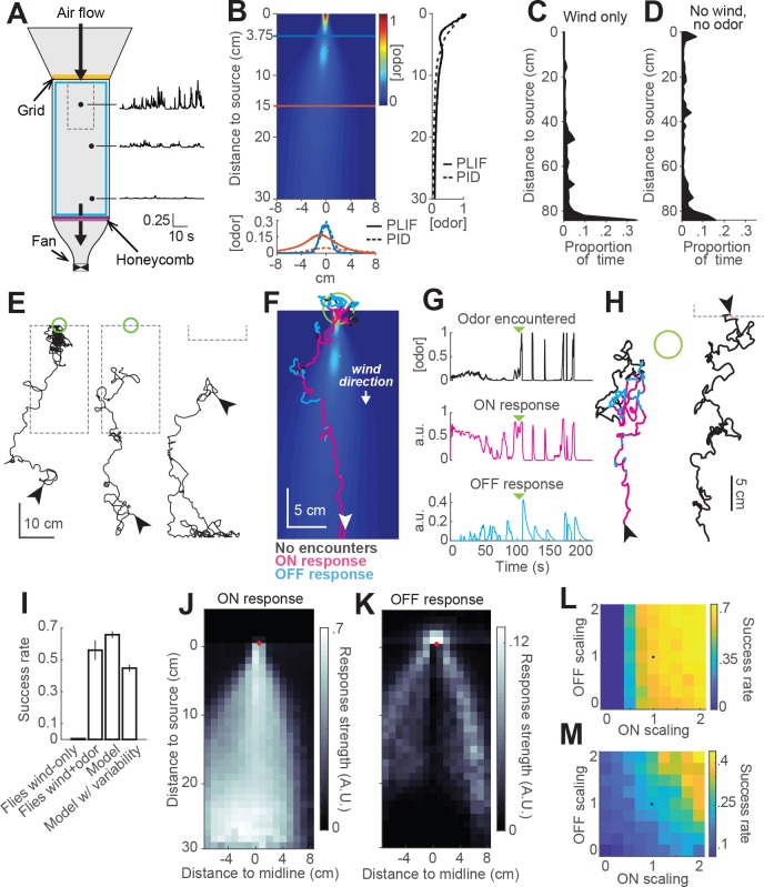
Figure 6. Real and virtual behavior of flies in a turbulent odor environment.

(A) Schematic of a turbulent wind tunnel used for behavioral experiments and PLIF imaging (top view; see Materials and methods). Black arrows: direction of air flow drawn by fan at downwind end; top arrow coincides with the tube carrying odor to the arena. Black dots and associated traces: sites of PID measurements (and corresponding signals; units normalized to mean concentration near the odor source). Smaller dashed square: Area covered with the PLIF measurements in the Colorado wind-tunnel (see Materials and methods). Yellow line: position of the wooden dowel grid. Purple line: position of the honeycomb filter. Blue square: perimeter moat filled with water. (B) PLIF measurements of an odor plume (average of 4 min of data). Blue/red horizontal lines: Sites of cross-sections (bottom plot). Bottom plot: cross-sections of the plume measured with PLIF (solid lines; 4 min average) and PID (dashed lines; 3 min average). Right plot: Odor concentration along midline of the plume (x = 0) measured with PLIF and PID (4 and 3 min average, respectively). All measurements in B appear normalized to average odor concentration at the source. (C–D) Flies exhibit a downwind preference in the turbulent wind tunnel. (C) Distribution of fly positions during trials with wind but no odor (n = 14 flies/trials). (D) Same as C, during trials with no wind (n = 13 flies/trials). (E) Example trajectories of flies during trials with an odor plume. From left to right: a successful trial in which the fly came within 2 cm of the source; intermediate trial in which the fly searched but did not find the source; failed trial where fly moved downwind. Arrowheads: starting positions. Green circles: 2 cm area around odor source. Dashed gray lines: area covered by PLIF measurements (use as positional reference; right-most trace shows only lower section of outline). (F) Example trajectory of a model fly that successfully found the odor source (background image from B). Colors show times when ON > 0.1 (magenta) or OFF > 0.05 (cyan). White arrowhead: Starting position and orientation. Green circle: 2 cm area around source. (G) Time courses of odor concentration encountered along the trajectory in F, with corresponding ON and OFF responses. Green arrowheads: time of entrance into the green circle. (H) Example trajectories of model flies (color code, green circle and arrowheads as in F). Left trace and green circle associated: intermediate trial where fly searched but did not find the source. Right trace: failed trial where fly moved downwind. Dashed line: lower section of the plume area. (I) Performance (proportion of successful trials$\pm$SE; see Materials and methods) of real and model flies in a plume. Data from real flies on trials with only wind (n = 13 flies/trials) and trials with wind and odor (n = 14 flies/trials). Model data using parameters fit to the mean fly in every trial (n = 500 trials; see Results). Model with variable ON and OFF scaling, reflecting variability in ON/OFF responses across individuals (n = 500 trials; see Results and Figure 1—figure supplement 2). (J–K) Average strength of ON (J) and OFF (K) responses as a function of position for model flies in the plume (data from simulation with mean parameters). Red dots: odor source. Note that ON is high throughout the odor plume, especially along its center, while OFF is highest at the plume edges. (L) Performance of the model in a plume (proportion of successful trials) with different scaling factors applied to ON and OFF responses. Black dot: performance of model using fitted values. (M) Same as L for model flies navigating a simulated odor gradient with a gaussian distribution and no wind (see Materials and methods).