Advanced error diagnostics of the CMAQ and Chimere modelling systems within the AQMEII3 model evaluation framework

Abstract

The work here complements the overview analysis of the modelling systems participating in the third phase of the Air Quality Model Evaluation International Initiative (AQMEII3) by focusing on the performance for hourly surface ozone by two modelling systems, Chimere for Europe and CMAQ for North America.

The evaluation strategy outlined in the course of the three phases of the AQMEII activity, aimed to build up a diagnostic methodology for model evaluation, is pursued here and novel diagnostic methods are proposed. In addition to evaluating the “base case” simulation in which all model components are configured in their standard mode, the analysis also makes use of sensitivity simulations in which the models have been applied by altering and/or zeroing lateral boundary conditions, emissions of anthropogenic precursors, and ozone dry deposition.

To help understand of the causes of model deficiencies, the error components (bias, variance, and covariance) of the base case and of the sensitivity runs are analysed in conjunction with timescale considerations and error modelling using the available error fields of temperature, wind speed, and NO_x concentration.

The results reveal the effectiveness and diagnostic power of the methods devised (which remains the main scope of this study), allowing the detection of the timescale and the fields that the two models are most sensitive to. The representation of planetary boundary layer (PBL) dynamics is pivotal to both models. In particular, (i) the fluctuations slower than ~ 1.5 days account for 70–85 % of the mean square error of the full (undecomposed) ozone time series; (ii) a recursive, systematic error with daily periodicity is detected, responsible for 10–20 % of the quadratic total error; (iii) errors in representing the timing of the daily transition between stability regimes in the PBL are responsible for a covariance error as large as 9 ppb (as much as the standard deviation of the network-average ozone observations in summer in both Europe and North America); (iv) the CMAQ ozone error has a weak/negligible dependence on the errors in NO₂, while the error in NO2 significantly impacts the ozone error produced by Chimere; (v) the response of the models to variations of anthropogenic emissions and boundary conditions show a pronounced spatial heterogeneity, while the seasonal variability of the response is found to be less marked. Only during the winter season does the zeroing of boundary values for North America produce a spatially uniform deterioration of the model accuracy across the majority of the continent.

1. Introduction

The vast majority of the research and applications related to the evaluation of geophysical models make use of aggregate statistical metrics to quantify, in some averaged sense, the properties of the residuals obtained from juxtaposing observations and modelled output (typically time series of the variable of interest). This practice is rooted in linear regression analysis and the assumption of normally distributed residuals and has been proven to be reliable when dealing with simple, deterministic, and low-order models. Led by the rapid pace of improved understanding of the underlying physics, the paradigm is, however, changed nowadays in that models have grown in complexity and non-linear interactions and require more powerful and direct diagnostic methods (Wagener and Gupta, 2005; Gupta et al., 2008; Dennis et al., 2010; So-lazzo and Galmarini, 2016).

Evaluation of geophysical models is typically carried out under the theoretical umbrella proposed by Murphy in the early 1990s for assessing the dimensions of goodness of a forecast: consistency (“the correspondence between forecasters’ judgments and their forecasts”), quality (“the correspondence between the forecasts and the matching observations”), and value (“the incremental benefits realised by decision makers through the use of the forecasts”) (Murphy, 1993). Since 2010, the Air Quality Model Evaluation International Initiative (AQMEII, Rao et al., 2011) has focused on the quality dimension - the one most relevant to science, according to Weijs et al. (2010) - of air quality model hind-cast products, aiming to build an evaluation strategy that is informative for modellers as well as to users.

Our claim is that the value of a model’s result depends strictly on the quality of the model that, in turn, depends on sound evaluation. The scientific problem of assessing the quality of a modelling system for air quality is tackled by Dennis et al. (2010) who distinguish four complementary approaches to support model evaluation-operational, probabilistic, dynamic, and diagnostic-which are also the four founding pillars of AQMEII. Several studies performed under AQMEII have focused on the operational and probabilistic evaluation (Solazzo et al., 2012a, b, 2013; Im et al., 2015a, b; Appel et al., 2012; Vautard et al., 2012) and more recently efforts have been expanded to the diagnostic aspect (Hogrefe et al., 2014; Solazzo and Galmarini, 2016; Kioutsioukis et al., 2016; Solazzo et al., 2017).

Operational metrics usually employed in air quality evaluation (see Simon et al., 2012, for a review) have several limitations as summarised by Tian et al. (2016): interdependence (they are related to each other and are redundant in the type of information they provide), under determination (they do not describe unique error features), and incompleteness (how many of these metrics are required to fully characterise the error?). Furthermore, they do not help to determine the quality problem set above in terms of diagnostic power. Gauging (average) model performance through model-to-observation distance leaves open several questions such as (a) how much information is contained in the error? In other words, what remains wrong with our underlying hypothesis and modelling practice? (b) Is the model providing the correct response for the correct reason? (c) What is the degree of complexity of the system models can actually match? These questions have a straightforward, very practical impact on the use of models, the return they provide (the value), and their credibility. Answers to these questions are also relevant to the widespread practice of bias correction, which aims to adjust the model value to the observed value rather than correct the causes of the bias which might stem from systematic, cumulative errors.

The main aims of this study are to move towards tools devised to enable diagnostic interpretation of model errors, following the approach of Gupta et al. (2008, 2009), Solazzo and Galmarini (2016), and Kioutsioukis et al. (2016), and to advance the evaluation strategy outlined in the course of the three phases of AQMEII. In particular, the work presented here is meant to complement the overview analysis of the modelling systems participating in AQMEII3 (summarised by Solazzo et al., 2017) by concentrating on the performance for surface ozone modelled by two modelling systems: Chimere for Europe (EU) and CMAQ for North America (NA). This study attempts to

• –identify the timescales (or frequencies) of the error of modelled ozone;
• –attribute each type of error to processes by utilising modelling runs with modified fluxes at the boundaries (anthropogenic emissions and deposition at the surface and boundary conditions at the bounding planes of the domain) and breaking down the mean square error (MSE) into bias, variance, and covariance - this analysis allows us to diagnose the quality of error and to determine whether it is caused by external conditions or due to missing or biased parameterisations or process representations;
• –investigate the periodicity of the ozone error which can be symptomatic of recursive (either casual or systematic) model deficiencies;
• –determine the role of the error of precursor or meteorological fields in explaining the ozone error. The significance (or the non-significance) of a correlation between the ozone error and that of one of the explanatory variables can help to understand the impact (or lack of impact) of the latter on the ozone error as well as the timescale of the process(es) causing the error.

Among the several models participating in AQMEII3, CMAQ and Chimere have been selected as the analysis proposed in this study requires additional simulations beyond those performed by all AQMEII3 groups, which implied additional dedicated resources that were not available to all groups. This of course opens an important issue connected with the relevance of models in decision making, the adequacy of their contribution, and consequently the fact that far more resources would be required by the present complexity and state of development of modelling systems to guarantee that deeper evaluation strategies are put in place. Although only these two modelling systems are analysed here, they represent two well-established systems that have been systematically developed over many years, are in use by a large number of research groups around the world, and also have participated in the various phases of AQMEII.

The data, model features, and error decomposition methodology are summarised in Sect. 2. Results of the aggregate time series and error decomposition analyses are presented in Sect. 3 and results of the diagnostic error investigation through wavelet, autocorrelation, and multiple regression analysis are presented in Sect. 4. Discussion, conclusions, and final remarks are drawn in Sects. 5 and 6.

2. Methods

2.1. Data and models

Unless otherwise specified, analyses are carried out and results are presented for the rural receptors of three subregions over each continental area as shown in Fig. 1. The three subregions have been selected based on similarity analysis of the observed ozone fluctuations slower than ~ 1.5 days. The regions where the slow fluctuations showed similar characteristics were selected through unsupervised hierarchical clustering (details in Solazzo and Galmarini, 2015). Due to the similarity of the observations within these regions, which implies that they experience common physical and chemical characteristics, spatial averaging within these subregions was carried out.

Figure 1.

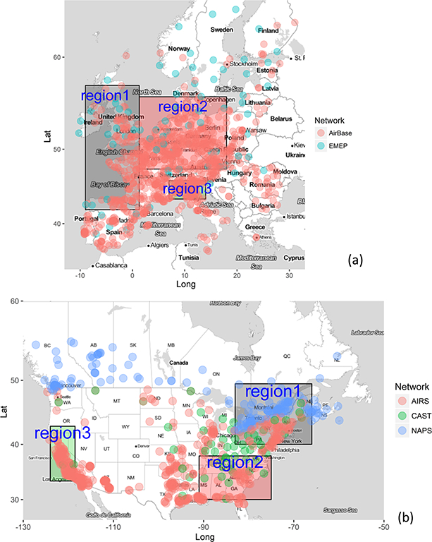
Continental domains and subregions used for analysis. The networks of ozone receptors are also shown.

The stations used for the analysis are part of European (European Monitoring and Evaluation Programme: EMEP; http://www.emep.int/; European Air Quality Database AirBase; http://acm.eionet.europa.eu/databases/airbase/) and North American (USEPA Air Quality System AQS: http://www.epa.gov/ttn/airs/airsaqs/; Analysis Facility operated by Environment Canada: http://www.ec.gc.ca/natchem/) monitoring networks. Full details are given in Solazzo et al. (2017) and references therein.

Following the approach used in previous AQMEII investigations, modelled hourly concentrations in the lowest model layer (~20 m for both models) and corresponding observational data are paired in time and space to provide a verification data sample {${\mathrm{mod}}_r^t$, ${\text{obs}}_r^t$; t = 1,..., 8760; r = 1,..., n_recs} of n_recs (number of monitoring stations) record of matched modelled and observational data, where the rth pair mod^t0 and obs^t0 is evaluated at receptor r at a given time t₀. Further, while the observations are reported at the hour at the end (for Europe) or at the beginning (for NA) of the hourly averaging window, the model values available in this study are provided instantaneously. Therefore, the model concentrations were assumed to be linear between the instantaneous on-the-hour reporting times; the integration (average) between those times was used to construct hour starting (or ending) values in order to more directly compare to the averaging used in the observations. This is of particular relevance when estimating the error due to timing of the diurnal cycle discussed in Sect. 4.3.

For the analyses conducted in this study, the spatial average of the observed and modelled ozone time series has been carried out prior to any time aggregation; i.e. the spatial average is created by averaging the hourly values over all rural stations in each region. Missing values in the time series, prior to the spatial averaging, have not been imputed. The analysis is restricted to stations with a data completeness percentage above 75 % and located below 1000 m above sea level. Time series with more than 335 consecutive missing records (14 days) have been also discarded. The number of rural receptors n_recs for ozone is 38, 184, and 40 for EU1, EU2, and EU3 and 73, 43, and 28 for NA1, NA2, and NA3, respectively. The EU continental domain used for analyses extends between −30 and 60° latitude and between 25 and 70° longitude, whereas the NA continental domain extends between-130 and-40° latitude and between 23.5 and 69° longitude.

The configuration of the CMAQ and Chimere modelling systems for AQMEII3 is extensively discussed in Solazzo et al. (2017) with respect to resolution, parameterisations, and inputs of emissions, meteorology, land use, and boundary conditions. For completeness a short summary is provided hereafter.

The CMAQ model (Byun and Schere, 2006) is configured with a horizontal grid spacing of 12 km and 35 vertical layers (up to 50 hPa) and uses the widely applied CB05-TUCL chemical mechanism (carbon bond mechanism; Whitten et al., 2010) for the representation of gas-phase chemistry. Emissions from natural sources are calculated by the Biogenic Emissions Inventory System (BEIS) model. The meteorology is calculated by the Weather Research and Forecast (WRF) model (Skamarock et al., 2008) with nudging of temperature, wind, and humidity above the planetary boundary layer (PBL) height. In CMAQ, dry deposition is used as a flux boundary condition for the vertical diffusion equation. A review of CMAQ dry deposition model as well as other approaches is provided in Pleim and Ran (2011).

Chimere (Menut et al., 2013) is configured with a grid of 0.25° (corresponding, approximately, to 25 km × 18 km over France), nine vertical layers (up to 500 hPa), and uses the Melchior2 chemical mechanism (Lattuati, 1997) for the representation of gas-phase chemistry. Natural emissions are calculated using the MEGAN model (Guenther, 2012). The hourly meteorological fields are retrieved from the Integrated Forecast System (IFS) operated by the European Centre for Medium-Range Weather Forecast (ECMWF). In Chimere the dry deposition process is described through a resistance analogy (Wesely, 1989). For each model species, three resistances are estimated: the aerodynamical resistance, the resistance to diffusivity near the ground, and the surface resistance. For particles, the settling velocity is added. More information is included in Menut et al. (2013).

Both models are widely used worldwide in a range of applications such as scenario analysis, forecasting, ensemble modelling, and model intercomparison studies.

2.2. Sensitivity runs with CMAQ and Chimere

The Chimere and CMAQ models have been used to perform a series of sensitivity simulations aiming for a better understanding of the causes of differences between the base model simulations and observed data. In particular, the following set of sensitivity runs was performed:

• –One annual run with zeroed anthropogenic emissions provided an indication of the amount of regional ozone due to boundary conditions and biogenic emissions (referred to as “zero emi”).
• –One annual run with a constant value of ozone (zero for NA and 35 ppb for EU) at the lateral boundaries of the model domain provided an indication of amount of ozone formed due to anthropogenic and biogenic emissions within the domain (in addition to the constant value for EU) (referred to as “zero BC” and “const BC”). All species other than ozone had boundary condition values of zero for both NA and EU in these sensitivity simulations.
• –One annual run was performed where the anthropogenic emissions are reduced by 20 %. In addition, the boundary conditions for this run were prepared from a C-IFS simulation (detail in Galmarini et al., 2017, and references therein) in which global anthropogenic emissions were also reduced by 20 % (referred to as a “20 % red”).
• –One run with ozone dry deposition velocity set to zero was available for the months of January and July (referred to as “zero dep”).

The analyses presented are not meant to intercompare the two modelling systems, as the CMAQ and Chimere models are applied to non-comparable contexts (different emissions, meteorology, and observational data). The response of each model to the changes in emissions, boundary conditions, and deposition needs to be interpreted independently.

2.3. Error diagnostic metric

To aid diagnostic interpretation, the mean square (or quadratic) error (MSE = E[mod—obs]²) is decomposed according to

$$\begin{gathered} \text{MSE}={\left(\overline{\mathrm{mod}}-\overline{\mathrm{obs}}\right)}^2+{({\sigma }_{\mathrm{m}}-{\sigma }_{\mathrm{o}})}^2+2{\sigma }_{\mathrm{m}}{\sigma }_{\mathrm{o}}(1-r) \\ ={\mathrm{bias}}^2+\mathrm{var}+\mathrm{covar}, \end{gathered}$$ (1)

where σ_m and σ_o are the modelled and observed standard deviation, var and covar are the variance and covariance operators, r is the linear correlation coefficient, and bias is the time averaged offset between the mean modelled and observed ozone concentration. The decomposition in Eq. (1) (and several variations of it), derived e.g. by Theil (1961), has been extensively discussed in Potempski and Galmarini (2009), Solazzo and Galmarini (2016), and Gupta et al. (2009). The first two moments (mean and variance) relate to the systematic error (unconditional bias) and variability (variance), respectively. All other differences between the statistical properties of modelled and observed chemical species (e.g. the timing of the peaks and autocorrelation features) are quantified by the correlation coefficient, i.e. in the covariance term (Gupta et al., 2009).

The MSE is a quadratic, parametric metric widely applied in many contexts and occurs because the model does not account for information that could produce a more accurate estimate. Put in an information theory context, the MSE provides a measure of the information about the observation that is missing from a Gaussian model centred at a deterministic prediction (Nearing et al., 2016). Ideally, the deviation of a perfect model from the observation should be zero or simply white noise (uncorrelated, zero mean, constant variance). Various flavours of MSE decomposition have been exploited in several geophysical contexts (Enthekabi, et al., 2010; Murphy, 1988; Wilks, 2011; Wilmott, 1981; Gupta et al., 2009), all stemming from the consideration that the bias, the variance, and the covariance characterise different (although not complementary and not exhaustive) properties of the error - accuracy, precision, and correspondence, respectively.

The relative contribution of each of the MSE components to the overall MSE is summarised by the Theil coefficients (Theil, 1961):

$$\begin{gathered} F_{\mathrm{b}}={\mathrm{bias}}^2/\mathrm{MSE} \\ {F}_{\mathrm{v}}=\mathrm{var}/\mathrm{MSE} \\ {F}_{\mathrm{c}}=\mathrm{covar}/\mathrm{MSE}. \end{gathered}$$ (2)

The overall MSE suffers from the limitations of the aggregate metrics discussed in the introductory section, lacking independence and explanatory power (Tian et al., 2016). When decomposed (e.g according to Eq. 1), however, the underdetermination issue is reduced and the MSE coefficients (Eq. 2) do offer diagnostic aid in interpreting the modelling error (Gupta et al., 2009).

3. Sensitivity analysis to emissions and boundary conditions perturbations

3.1. Aggregated time series of ozone

Figures 2 and 3 show monthly and diurnal curves for the base and sensitivity simulations over the three subregions in each continent. Results show that the monthly averaged curves of the zeroed emission runs peak in April in NA and in July in EU (May to July in EU1 are approximately the same), indicating the periods when the impact of background concentration (boundary conditions) and biogenic emissions on regional ozone is largest: springtime in NA and summer in EU. The monthly curves of “zero BC” and “zero emi” for NA are anticorrelated between the months of April to July-August (“zero emi” curve decreasing and “zero BC” curve raising) and during autumn (“zero emi” curve rising and “zero BC” curve decreasing), framing the interplay among these two factors in terms of total ozone loading: boundary conditions dominate in autumn-winter and biogenic plus anthropogenic emissions are more important during spring-summer. The springtime peak for the zero emissions case over NA is consistent with the springtime peak in northern hemispheric background ozone (Penkett and Brice, 1986; Logan, 1999) and the predominant westerly and north-westerly inflow into the NA domain. The background ozone springtime peak is thought to be caused by a combination of more frequent tropospheric-stratospheric exchange and in-situ photochemical production during that season (Atlas et al., 2003).

Figure 2.

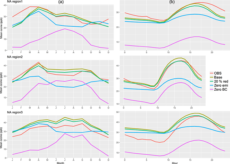
Average monthly (column a) and diurnal curves (column b) constructed from the January-December 2010 time series of hourly ozone observations and model simulations for three North American subregions.

Figure 3.

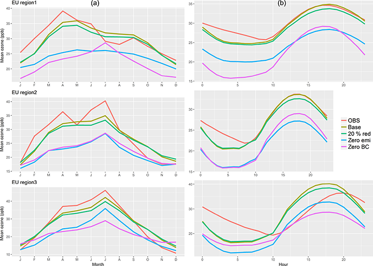
Average monthly (column a) and diurnal curves (column b) constructed from the January-December 2010 time series of hourly ozone observations and model simulations for three European subregions.

The daily averaged profiles of mean ozone for NA show that the observed peak (occurring between 16:00–18:00 LT in NA1 and NA2 and ~ 1 h earlier in NA3) is preceded by the peak in the base run by ~ 1 h in NA2 and by ~ 2–3 h in NA1, while the timing of the observed minimum (occurring at 08:00–09:00 LT) is captured by the base run in NA2 and NA3 while it is preceded by the base run by ~ 1 h in NA1. The modelled morning transition to convective conditions is in phase with the observations except for NA1, where the modelled transition occurs 1 h earlier than the observed one. The modelled afternoon transition in NA1 precedes the observed transition by 3–4 h, possibly due to errors in the partitioning between sensible and latent surface heat flux that causes a faster-than-observed collapse of the PBL. One possible reason, as discussed in Appel et al. (2017), could reside in the stomatal conductance function and the heat capacity for vegetation in WRF and the ACM2 vertical mixing scheme in both WRF and CMAQ (relative to the version of WRF and CMAQ used in the current study). Recent updates to these processes in CMAQ lead to a change in the modelled diurnal cycle of ozone as well as other pollutants and meteorological variables. In particular, the updates lead to a delay in the evening collapse of the modelled PBL (Appel et al., 2017).

The shape of the “zero BC” curve is similar in amplitude to that of the base run, suggesting that the effect of the regional/background ozone represented through boundary conditions in a limited area model is mainly to shift the mean concentration upwards, while it has no major effect on the frequency modulation. By contrast, the absence of anthropogenic emissions has a major effect on the amplitude of the signal as well as its magnitude (“zero emi” curve). As discussed in the next section, these considerations translate into the bias and/or variance type of error due to the boundary conditions and emissions.

As for EU (Fig. 3), the observed daily profiles in EU1 and EU2 are closely matched by the Chimere model between 11:00 and 23:00 LT (underestimated outside these hours), while in EU3 the daily peak (observed at 19:00–20:00 LT) is consistently occurring earlier in the model and its magnitude is overestimated. The morning transition occurs earlier in the model than the observations and follows a significant model underprediction of nighttime and early morning ozone due to difficulties in reproducing stable or near-stable conditions (Bessagnet et al., 2016). In EU3, the model displays the poorest performance, with significant underestimation between midnight and 09:00 LT (5–7 ppb) and overestimation in daylight conditions (7–9 ppb).

As opposed to the CMAQ case for NA, the shape of the “zero emi” curve of Chimere closely follows the shape that of the base case (even when considering only the stations classified as “urban”; Fig. S2 in the Supplement). Due to the long time average (1 year), the daily profiles displayed in Figs. 2 and 3 do not provide information about the exact timing of the minima and maxima for each season throughout the year. Figures S3 and S4 report the seasonal average diurnal profiles for the model predictions and the observations (network average over all stations) and show that the timing of the ozone diurnal cycle varies seasonally.

3.2. Error decomposition

The plots in Figs. 4 (NA) and 5 (EU) show the MSE decomposition according to Eq. (1) for the summer months of June, July, and August for the base case simulation as well as the sensitivity simulations, distinguishing between daylight (from to 05:00 to 09:00 LT) and nighttime hours (the remaining hours, from 10:00 to 04:00 LT). These plots are meant to aid the understanding of the relative impacts of potential errors in lateral boundary conditions, anthropogenic emissions, and the representation of ozone dry deposition on the total model error by comparing the magnitude and type of model error from these simulations against the model error for the base case.

Figure 4.

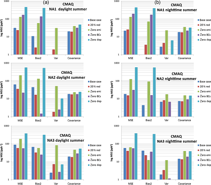
MSE decomposition for June-August hourly ozone into bias, variance, and covariance for the three North American (NA) subregions. Results are presented separately for daylight hours (a) and nighttime hours (b).

The plots in Figs. 6 to 15 are complementary to Figs. 4 and 5 and show the error decomposition for both the summer and winter season in more detail, including the error coefficients F_b, F_v, and F_c of Eq. (2) (left vertical axis), the total MSE (right vertical axis), the sign of the bias and variance error (± for model over- and underprediction), and the values of the correlation coefficient. Furthermore, the maps in Figs. 16 and 17 show the root MSE (RMSE) at the receptors for the “base” case as well as ΔRMSE, i.e. the percentage change of RMSE of the sensitivity runs with respect to the “base” case simulation:

$$\Delta \mathrm{RMSE}=100\cdot ({\mathrm{RMSE}}_s-{\mathrm{RMSE}}_{\mathrm{base}})/{\mathrm{RMSE}}_{\mathrm{base}},$$

where the subscript s indicates the zeroed emission or the zeroed (constant) boundary condition simulations (ΔRMSE is measured as percentage).

Figure 6.

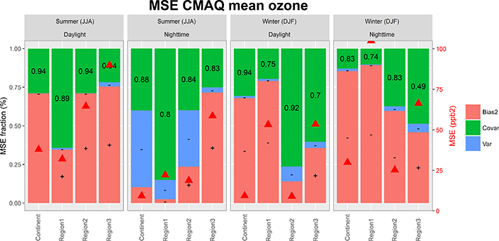
CMAQ MSE breakdown for summer and winter for the base case (hourly time series of ozone) over NA. The error coefficients F_b, F_v, and F_c are reported on the left axis and the total MSE (ppb²) on the right axis (red triangles). The + and — signs within the bias and variance portions of the errors indicate model over- and underprediction of mean concentration or variance, respectively. The values in the covariance portion indicate the correlation coefficient between modelled and observed time series. Results are provided separately for daytime and nighttime.

Figure 5.

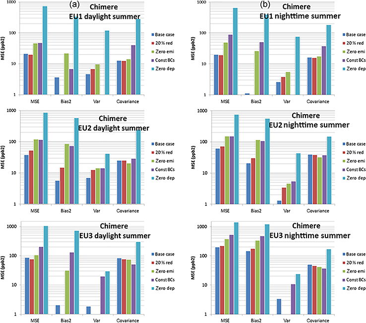
MSE decomposition for June-August hourly ozone into bias, variance, and covariance for the three EU subregions (the zero dep data refers to the month of July only). Results are presented separately for daylight hours (a) and nighttime hours (b).

Figure 16.

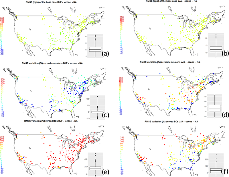
(a, b) Spatial maps of RMSE (in ppb) for the base case. (c, d) Percentage RMSE changes for the zeroed emissions case with respect to the base case. (e, f) Percentage RMSE changes for the zeroed boundary condition case with respect to the base case. (a, c, e) Winter months (DJF); (b, d, f) summer months (JJA).

Figure 17.

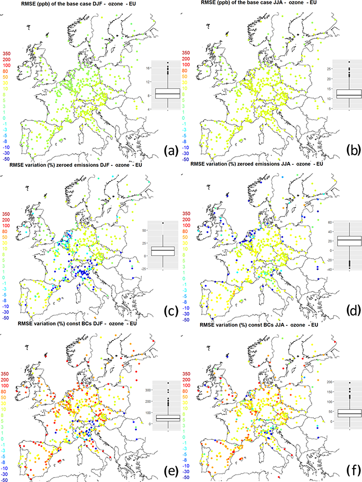
(a, b) Spatial maps of RMSE (in ppb) for the base case. (c, d) Percentage RMSE changes for the zeroed emissions case with respect to the base case. (e, f) Percentage RMSE changes for the constant boundary condition case with respect to the base case. (a, c, e) Winter months (DJF); (b, d, f) summer months (JJA).

The CMAQ results for NA are presented in Figs. 4, 6–10, and 16 and can be summarised as follows:

• –The MSE of the base case (MSE_base) during summer daylight is mainly due to bias (~35 % in NA1 and ~75 % in NA2 and NA3) and the remaining portion is due to covariance error. The fact that there is no variance error shows that the model is able to replicate the observed 3-month averaged variability. Possible reasons for the positive model bias (model overestimation) have been discussed in Solazzo et al. (2017) and includes overestimation of emissions precursors (Travis et al., 2016) and absence of correct parameterisations of forested areas on surface ozone (Makar et al., 2017).
• –The effect of zeroing the emissions of anthropogenic pollutants on the summer MSE is a rise by a factor ~2 to 4 (daylight) and by a factor ~6 to 7 (nighttime) in NA1 and NA2 with respect to MSE_base; during night-time in NA3 the MSE stays approximately the same, indicating that the emissions play a negligible role in determining the total error in this subregion during summer night.
• –Furthermore, all the error components deteriorate in the simulations with zero anthropogenic emissions except for the bias in NA3. This is particularly true for the variance, signifying the fundamental role of emissions in shaping the diurnal variation of ozone. Indeed, this suggests that the absence of a variance error in the base case (see above) is due to the correct interplay between the temporal/spatial distribution of the emissions, potentially coupled with the variability due to the meteorology.
• –The covariance share of the error also increases (although only slightly in NA2) for the zero emissions case, indicating that the emissions play a role in determining the timing of the modelled diurnal ozone signal; this increase is more pronounced during nighttime.
• –The zeroing of the input of ozone from the lateral boundaries has either no effect or only a limited effect (e.g. daylight summer in NA2; Fig. 4) on the variance and covariance shares of the error, while it has a profound impact on the bias portion. This impact is approximately equal during daylight and nighttime, as expected from the discussion of the daily cycle shown in Fig. 2.
• –The removal of ozone dry deposition from the model simulations (results based on July only) has the most profound impact, increasing by 1 order of magnitude the MSE of the base case, which is approximately double the combined effect of the emissions and boundary conditions perturbation. This sensitivity gives a gross indication of the relative strength of this process vs. external conditions during summer, while the “zero BC” case has a larger effect than the “zero deposition” case in January (not shown). Similar to the “zero BC” case, the exclusion of ozone dry deposition from the model simulations acts as an additive term to the diurnal curve in NA1, leaving almost unaltered the shape and timing of the signal, while it impacts the variance and covariance error in the other two subregions. The small impact the removal of dry deposition has on the covariance error (timing of the ozone signal) together with the outweighing offsetting bias might suggest that the correct estimate of the deposition magnitude is more beneficial than, e.g. the time dependence of surface resistance. The role of the variance is, however, unclear and deserves further analyses.
• –The instances where the “20 % red” bias error is lower than the error of the base case occur when the mean ozone concentrations were overestimated in the base case (e.g. daylight for all subregions and NA2 and NA3 over nighttime summer) as illustrated in Figs. 6 and 7.
• –The maps show that there are stations where the error is reduced with zero anthropogenic emissions (e.g. a reduction of 20–30 % in the southern coast of the US and in the far north-east during summer; Fig. 16d). This suggests the presence of other compensating model errors in both the base and sensitivity simulations that lead to better agreement with observations when prescribing an unrealistic emission scenario. The sources of these compensating errors need to be investigated in future work.
• –The “zero BC” run has profound negative effects over the whole continental area of NA during winter (Fig. 16e), while the effects are smaller during summer (Fig. 16f), especially over the southern coast, due to the relatively higher importance of photochemical formation of ozone during summer.
• –The error characteristics of the daily maximum 8 h rolling mean (DM8h, Fig. 10) resemble those of the daylight base case (Fig. 6, left column), but reduced in magnitude during winter, with almost null variance error and the same sign of the bias as the base case. The NA1, NA2, and NA3 standard deviations of the summer DM8h is of 7.6, 5.2, and 8.1 ppb and of 7.6, 6.5, and 7 ppb for the model and the observations, respectively. The model variability is therefore in line with the observed variability. The error of the DM8h for the sensitivity runs is reported in Fig. S5.
• –On a network-wide average, removing anthropogenic emissions causes a RMSE increase of 25 % during summer and of 0 % (10 % at 75th percentile) during winter while a zeroing out of input from the lateral boundaries causes a RMSE increase of 30 % during summer and of 180 % during winter (median values; Fig. 16)

Figure 10.

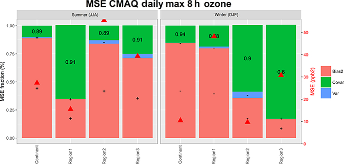
As in Fig. 6 for the rolling average daily maximum 8 h ozone time series.

Figure 7.

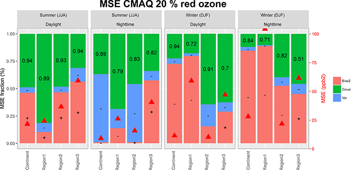
As in Fig. 6 for the hourly time series of “20 % reduction” scenario.

The allocation of the error of the Chimere model for EU varies greatly by subregion (Figs. 5, 11–15, and 17):

• –The summer daylight RMSE_base ranges between ~ 20ppb² (EU1, ~ 60% covariance and ~20% bias) and ~85ppb² (EU3, 95% covariance). In EU3, the nighttime bias of ~75 % outweighs the covariance, as seen in Fig. 11.
• –Removing the anthropogenic emissions had almost no effect on the covariance share of the MSE (if not a slight reduction with respect to the base case in EU2 and EU3 and also during nighttime), indicating that the error in the timing of the signal is influenced not by the emissions but rather by other processes. Moreover, the variance portion is left almost unchanged (1 ppb increase in EU1 and EU2), in contrast to the CMAQ results for NA. This would indicate that the variability of ozone concentration is hardly influenced by anthropogenic emissions in Chimere. The bias is the error component most sensitive to emissions reductions, especially in EU2 and less so in EU3. This is in line with the discussion of the daily profiles of Fig. 2b (which showed similar shapes of for the “zero emi” and of the “base” profiles) and contrasts with the NA case where the “zero emi” daily profiles are flatter than the base case.
• –The effect of imposing a constant ozone boundary condition value of 35 ppb (and of zero for all other species) has a net small effect on the variance of the ozone error but significantly reduces the covariance share of the error in favour of the bias (Figs. 5 and 14). The total MSE is similar to that of removing the anthropogenic emissions as far as the total MSE and the bias of EU2 are concerned. It outweighs the latter for the total MSE, bias, and variance in EU3 and covariance and nighttime bias component in EU1. We can infer that the variability of the boundary conditions has a significant role in determining the timing of the ozone signal in EU1 (close to the western boundary of the domain) as the correlation coefficient degrades from 0.89 (base case) to 0.66 (“const BC”) (Figs. 5, 11, and 14). The bias staying the same in EU1 daylight summer depends on the magnitude of the constant value (35ppb were chosen here) that is in close agreement with that of the base case while the small variance error (~2 ppb) vanishing with respect to the base case might be explainable with numerical compensation.
• –During summer in EU2 and EU3 changing the ozone boundary condition only influences the bias with marginal impacts on variance and covariance, while in winter (Fig. 14) there is also a significant reduction of the correlation coefficient, meaning that the boundary conditions modulate the timing of the signal. This also implies that the variability of the boundary conditions becomes more important in winter.
• –EU3 deserves special consideration as the RMSE_{zero emi} is approximately the same as the RMSE_base, which mostly consists of covariance error during daylight and bias error during nighttime (Fig. 5e). Due to the local topography, EU3 is typically characterised by stagnant conditions that are difficult to model. For example, 50 % of the observed wind speed is below 1.65ms⁻¹, while Chimere predicts 1.95 ms⁻¹. The largest impact on the total MSE is seen in the “const BC” run and arises in the bias portion, pointing to the importance of properly characterising background (regional) concentrations.
• –With respect to the base case, the DM8h (Fig. 15) shows a reduced share of the covariance error with respect to the mean ozone (Fig. 11) at the expense of an increase in variance error; the timing error is now shifted towards seasonal timescales. The variability of the DM8h is governed by synoptic processes which are likely responsible for the variability error of the DM8h. The EU1, EU2, and EU3 standard deviations of the summer DM8h is of 3, 6.2, and 8.6ppb and of 6, 11, and 10.2ppb for the model and the observations, respectively. The model therefore underestimates the observed variability (as indicated by the “minus” sign in the variance share of the error in Fig. 15) by up to 50 % in EU1. A range of processes could be responsible for the lack of variability in Chimere, from emission to chemistry to transport. The error of the DM8h for the sensitivity runs is reported in Fig. S6.
• –On a network-wide average, removing anthropogenic emission causes an RMSE increase of 21 % during summer and 12 % during winter (median values; Fig. 17c,d).
• –The effect of setting the dry deposition velocity of ozone to zero (July only, Fig. 5) increases not only the bias error but also the variance and covariance shares of the error. Thus in Chimere the deposition not only acts as a shifting term on the modelled concentration but also influences the variability and timing of ozone more profoundly than for the CMAQ case examined earlier.

Figure 11.

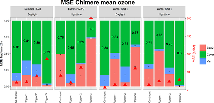
Chimere MSE breakdown for summer and winter for the base case (hourly time series of ozone) and sensitivity simulations over EU. The error coefficients F_b, F_v, and F_c are reported on the left axis, the total MSE (ppb²) on the right axis (red triangles). The + and — signs within the bias and variance portions of the errors indicate model over- and underprediction of mean concentration or variance, respectively. The values in the covariance portion indicate the correlation coefficient between modelled and observed time series. Results are provided separately for daytime and nighttime.

Figure 15.

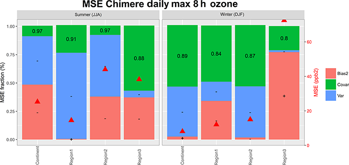
As in Fig. 11 for the rolling average daily maximum 8 h ozone time series.

Figure 14.

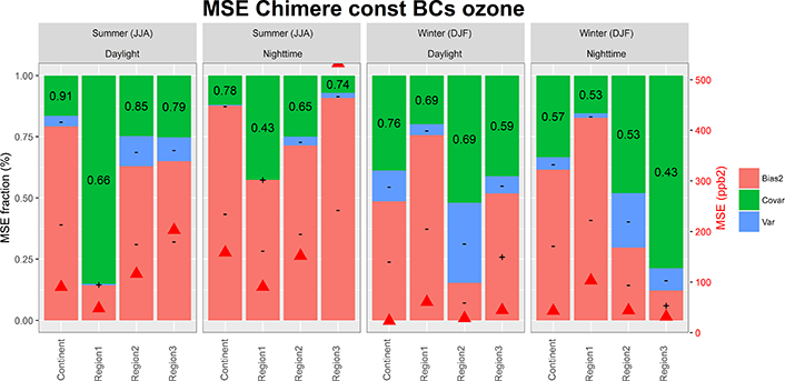
As in Fig. 11 for the hourly time series of the “constant boundary conditions” scenario.

4. Timescale error analysis and diagnostic

The focus of this section is ΔO₃, the time series of the deviation between the base case and observations. The nature of ΔO₃ is examined for time-frequency patterns using wavelet analysis and for error persistence using autocorrelation functions (ACFs). The causes of ΔO₃ are also tentatively investigated as dependencies on other fields using multiple regression analysis combined with bootstrapping to sample the relative importance of the regression variables.

4.1. Spectral considerations

The coefficients of the ACFs (Appendix A) can be interpreted as the Fourier transform of the power spectral density. Frequency analysis of a signal is often performed by constructing the periodogram (or spectrogram; see e.g. Chat-field, 2004). This approach has proven useful when dealing with harmonic processes superimposed on a baseline signal (Mudelsee, 2014) but, at the same time, periodograms often contain high noise. Therefore, examining a signal at specific frequencies can be instructive, for instance by resorting to wavelet transform, which has the further advantage of enabling a 3-D time-frequency-power visualisation. Compared to a power spectrum showing the strength of variations of the signal as function of frequencies, wavelet transformation also allows the allocation of information in the physical time dimension other than phase space. Here, wavelet analysis of the periodogram of seasonal ΔO₃ is performed using the Morlet wavelet transform (Torrence and Compo, 1997).

From inspecting Fig. 18 (NA) it emerges that the highest values of spectral energies for ΔO₃ for the three subregions (corresponding to the 99th percentile of the spectrum) are observed for periods spanning the whole year (i.e. the intensity keeps the same high value during the whole year and is associated with a periodicity higher than ~300 days). These high values of the energy spectrum are likely associated with the slow variability of the non-zero bias throughout the investigated period that acts as a slow envelop modulation of the error at shorter timescales. Such a process is more evident in NA1 and NA2 and its magnitude is 1 order of magnitude (or more) higher of the 90th percentile value.

Figure 18.

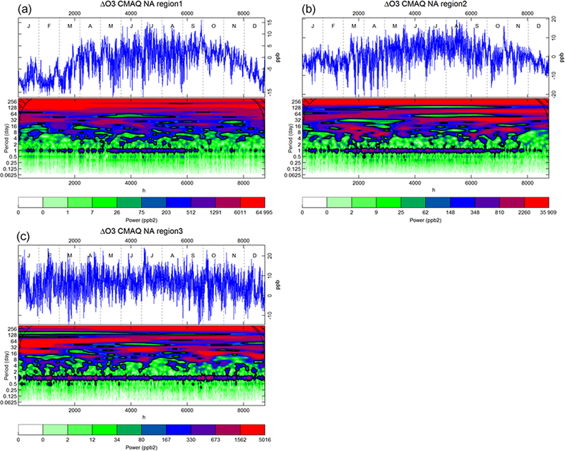
Annual time series of differences between CMAQ and observed O₃ (ΔO₃, top portion of each panel) and Morlet wavelet analysis of the periodogram of ΔO₃ (lower portion of each panel) for the three NA subregions. Black contours lines identify the 95 % confidence interval. The period (in days) is reported in the vertical axis, while the quantiles of the power spectral density are measured in ppb². (The scale reports the quantiles of the power spectrum.)

NA3 and to a lesser extent NA2 show a high spectral power of the error for periodicities of 1–2 months and lasting from January to May with a weaker wake extending up to the end of the year, potentially pointing to errors in the characterisation of larger-scale background concentrations associated with boundary conditions. NA3 also exhibits a high spectral power for errors associated with a periodicity of ~20 days during January-February and June-July and ~15 days during October and December. This may point to errors in representing the effects of changing weather regimes on simulated ozone concentrations.

Except for the long-term variations of the model error with periodicities greater than 2 months discussed above, NA1 is the only subregion that shows only weak power associated with model errors of shorter periodicities from June to December. This suggests that fluctuations caused by variations in large-scale background and changing weather patterns are better captured in this region compared to the other two subregions.

The energy associated with the daily error is again higher and more pronounced in NA3 than in the other subregions, where it is most pronounced during summer (NA1) or between March to October (NA2). While during winter and autumn the daily error is likely driven by difficulties in reproducing stable PBL dynamics, during spring and summer it is also influenced by the chemical production and destruction of ozone, a process entailing NO_x chemistry, radiation, biogenic emission estimates, and chemical transformation, and thus difficult to disentangle from boundary layer dynamics. Wavelet plots of the ozone error for periods between 12 h and 6 days are reported in Figs. S7 and S8, allowing us to better identify the periods (and/or the periodicity) affecting the error of the fast fluctuations, e.g the daily error in NA3 (all year) and the high energy spot towards the end of April in NA2 with a periodicity of ~6 days and above, that could be associated with an ozone episode, but analysis of episodes is beyond the scope of this investigation.

For the EU (Fig. 19) a notable feature is the very high daily error energy in EU3 that is present throughout the year and most pronounced in summer. Such high energy suggests persistent problems in representing processes having a periodicity of 1 day. Further, EU3 shows an area of high energy associated with a period of 1 to 2 months and extending from February, peaking in April and May, and ending in September (mostly model underestimation; Fig. 19c), while the error of the winter months in EU3 receives high energy from slower processes, acting on timescales of ~6 months and beyond. Considering that the EU3 region is surrounded by high mountains, tropopause folding (e.g. Bonasoni et al., 2000; Makar et al., 2010) together with the lack of modelling mechanisms for the tropopause/stratosphere exchange could offer an explanation of the high energy of the error at long timescales (also considering that the higher level modelled by Chimere is well below the tropopause and that vertical fluxes are those prescribed by the C-IFS model). Errors in the biogenic emissions also remain a plausible cause of ozone error during spring and summer months.

Figure 19.

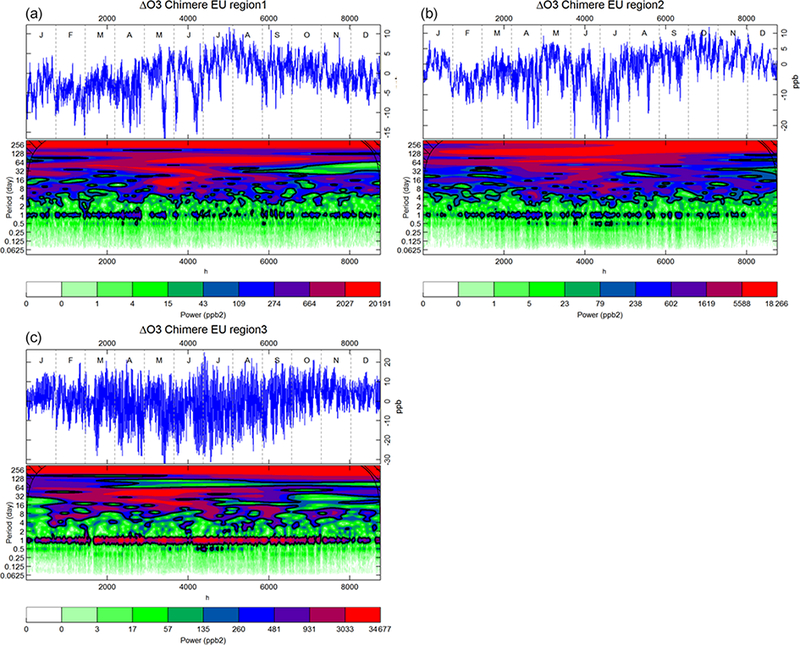
Same as in Fig. 18 for Chimere over the three EU subregions.

The similarity of the wavelet spectra for NA3 (Fig. 18c) and EU1 (Fig. 19a) (both regions are located on the western edge of their domain) at the beginning of the year for periods of 1 to 2 months might be indicative of the periodicity of the bias induced by the boundary conditions. Compared to CMAQ, the error of the Chimere model is more concentrated during spring and early summer, with a periodicity of 10–20 days.

Having identified some relevant timescales for the ΔO₃ error, in the next sections methods are proposed for its detection and quantification.

4.2. Temporal characteristics of the error of ozone

In a recent study, Otero et al. (2016) analysed which synoptic and local variables best characterise the influence of large-scale circulation on daily maximum ozone over Europe. The authors found the majority of the variance during spring over the entire EU continent is accounted for in the 24 h lag autocorrelation while during summer the maximum temperature is the principal explanatory variable over continental EU. Other influential variables were found to be the relative humidity, the solar radiation, and the geopotential height. Camalier et al. (2007) and Lemaire et al. (2016) found that the near-surface temperature and the incoming short-wave radiation were the two most influential drivers of ozone uncertainties.

The ACFs and PACFs (partial autocorrelation function) of ΔO₃ (see Appendix A for a definition of both functions) reveal a strong periodicity for periods that are multiples of 24 h (Figs. 20 and 22) (note that the first derivative of ΔO₃ is used in this analysis to achieve stationarity). The structure of the error is such that it repeats itself with daily regularity, indicating either a systematic error in the model physics or a missing process at the daily scale, possibly related to radiation and/or PBL-related variables. While the presence of a daily periodic forcing due to the deterministic nature of day-night differences superimposed on the baseline ozone is expected, the periodicity maintained in the error structure is not and deserves further analysis.

Figure 20.

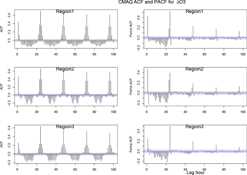
CMAQ model: autocorrelation (ACF) and partial autocorrelation (PACF) functions for the differenced time series of residuals of ozone (model-observations). The differentiation is necessary to remove non-stationarity and thus to convey the ACF and PACF values depending on lag only.

Figure 22.

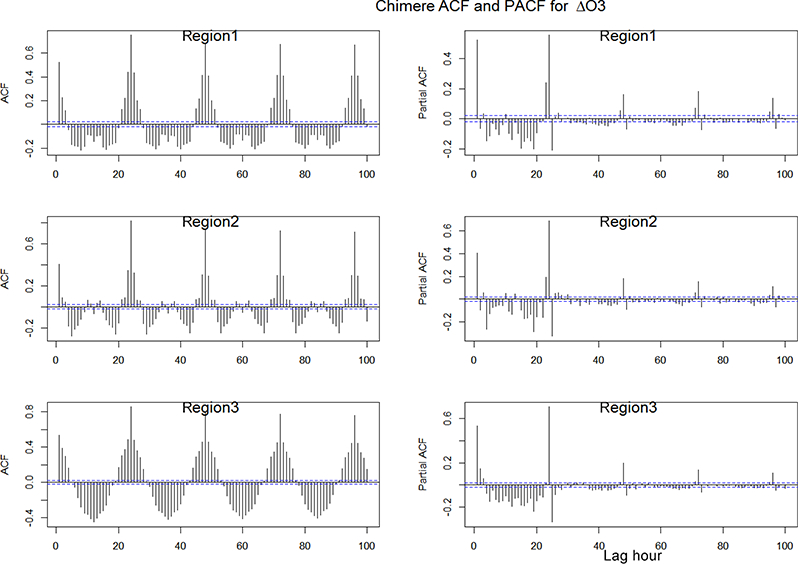
Chimere model: autocorrelation (ACF) and partial autocorrelation (PACF) functions for the differenced time series of residuals of ozone (model-observations). The differentiation is necessary to remove non-stationarity and thus to convey the ACF and PACF values depending on lag only.

The PACF plots confirm that the error is not simply due to propagation and memory from previous hours but rather arises at 24 h intervals and hence stems from daily processes. On average, for NA corr(ΔO₃ (h), Δ0₃(h+1)) (i.e. the correlation between ΔO₃(h) and ΔO₃(h+1)) is ~0.45, while the corr(ΔO₃(h), ΔO₃(h+24) ~0.68, for any given hour h. Similarly for EU, corrΔO₃(h) and ΔO₃(h+1)) ranges between 0.31 (EU2) and 0.54 (EU3), while corrΔO₃(h), ΔO₃(h+24)) ~0.70 for all subregions. Thus, the ozone error with a 24 h periodicity has a longer memory than the error with a 1 h periodicity. Since the 24 h periodicity of the error is present in the entire annual time series, the periodic error is not associated with particular conditions (e.g. stability) but is rather embedded into the model at a more fundamental level. Moreover, similar periodicity is observed for

• –the ACF analysis repeated for the “zero emi” scenario (Fig. S9);
• –the ACF of ΔWS and ΔTemp for both models (Fig. S10);
• –the ACF of primary species (PM₁₀ for EU and CO for NA) (Fig. S11);
• –the ACF of ozone error for the “zero emi” scenario at three stations where isoprene emissions are low (Fig. S12). These stations have been selected by looking at the locations where isoprene emissions accumulated over the months of June, July, and August as provided by the two models analysed here.

In all cases, the error has a marked daily structure, strengthening the notion that a daily process affecting several model modules is not properly parameterised. The error due to chemical transformation at daily scale is screened out by the daily periodicity of the ACF of the primary species, while the daily periodicity of the zeroed emission scenario allows the reinforcement of the claim that the PBL dynamics is the most probable cause of the error.

Since the individual daily processes directly or indirectly affecting the PBL dynamics cannot be untangled, here “PBL error” is meant to encompass errors in the representation of the variables affecting boundary layer dynamics (i.e. radiation, surface description, surface energy balance, heat exchange processes, development or suppression of convection, shear generated turbulence, and entrainment and detrainment processes at the boundary layer top for heat and any other scalar) and their non-linear interdependencies.

By removing the diurnal fluctuations (i.e. by screening out the frequencies between 12 h and up to ~1.5 days by means of the Kolmogorov-Zurbenko (KZ) filter, as described in Hogrefe et al., 2000) from the modelled and observed time series, the daily structure of the ACF disappears (Figs. 21 and 23), replaced by a slow decay and negative (EU1, EU2 and partially NA1, NA2) or fluctuating (NA3, EU3) correlation values. The PACF plots in Figs. 21 and 23 suggest that some significant correlation persists up to ~40 h, likely due to leakage from the removed diurnal component. As extensively discussed in several earlier works, the KZ filter does not allow for a clear separation among components and thus some leakage is expected (see e.g. Galmarini et al., 2013; Solazzo et al., 2017). The amount of overlapping variance between the isolated diurnal fluctuations and the remainder of the time series is of ~4–9%.

Figure 21.

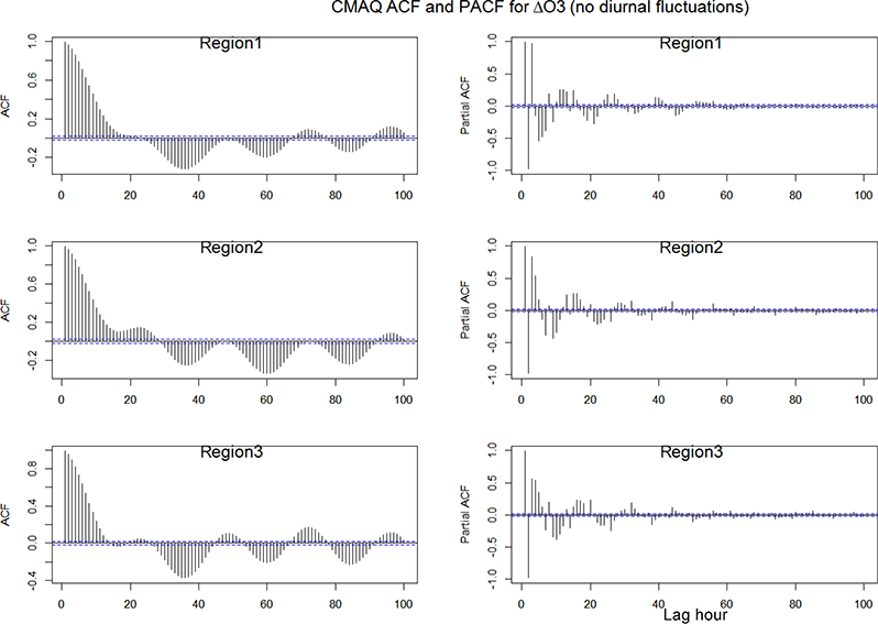
As in Fig. 20 for the differenced time series of residual of ozone obtained by filtering out the diurnal fluctuations from the modelled and observed time series.

Figure 23.

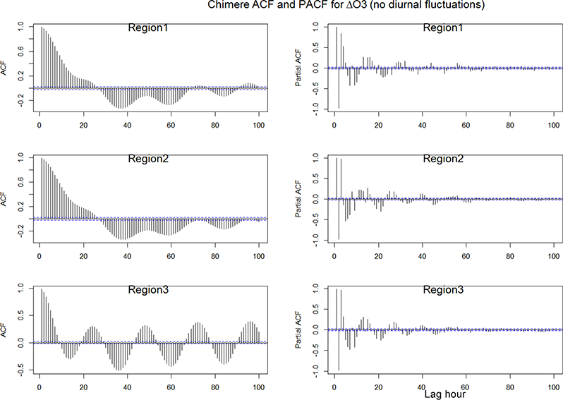
As in Fig. 22 for the differenced time series of residual of ozone obtained by filtering out the diurnal fluctuations from the modelled and observed time series.

The relative strength of the MSE for the undecomposed ozone time series and for the ozone time series with the diurnal fluctuations removed and with only the diurnal fluctuations is reported in Table 1. With the exception of NA1 and EU3, the baseline error (denoted with “noDU”) accounts for ~70 to 85 % of the total error, while the diurnal fluctuations (denoted with “DU”) are responsible for 10 to 23 % of the total error (and even less during nighttime). The “DU” error outweighs the “noDU” error (67% to 26%) only in EU3, where the daily PBL issue has been pointed out in the previous section.

Table 1.

MSE (ppb²) of the full, undecomposed ozone time series (FT) and relative fraction of MSE of the time series derived by filtering out the diurnal fluctuations (noDU) and of the time series derived by keeping only the diurnal fluctuations (DU). The diurnal signal has been isolated by applying a Kolmogorov-Zurbenko filter KZ(13,5). The relative fraction of noDU and of DU does not add up to 100% because the filter allows some leakage to the nearest frequencies (see Hogrefe et al., 2000, and Solazzo and Galmarini, 2016, for details). (a) NA; (b) EU.

(a)	NA1			NA2			NA3			Continent
	FT (ppb2)	noDU	DU	FT (ppb2)	noDU	DU	FT (ppb2)	noDU	DU	FT (ppb2)	noDU	DU
CMAQ MSE - summer
	28.65	40%	41 %	49.12	70%	23%	79.35	84%	13%	28.25	56%	29 %
CMAQ MSE - winter
	86.08	94%	5%	19.27	75 %	21%	61.67	74%	21 %	22.38	85%	9%
(b)	EU1			EU2			EU3			Continent
	FT (ppb2)	noDU	DU	FT (ppb2)	noDU	DU	FT (ppb2)	noDU	DU	FT (ppb2)	noDU	DU
CHIMERE MSE - summer
	20.91	85%	10%	46.19	78 %	15%	125.86	26%	67 %	26.95	76%	18%
CHIMERE MSE - winter
	20.87	85%	12%	19.95	85%	10%	39.91	38 %	59%	11.34	73%	16%

4.3. Covariance error: phase shift of the diurnal cycle

This section explores the nature of the covariance error which occurs, among other reasons, when the two signals being compared are not in phase. The first and second moments of the error distribution are invariant with respect to a phase shift between the two signals (Murphy, 1995); i.e. the mean of the signal and the amplitude of the oscillations with respect to the mean value are not affected by a phase shift, which therefore does not have an impact on the bias and variance components of the error. The correlation coefficient, in contrast, is impacted by a lagged signal, producing a net increase of the covariance error.

The analysis of the phase lag between the daily component of the modelled and observed cycles is reported in Figs. 24 (NA) and 25 (EU), while winter and summer are analysed separately.

Figure 24.

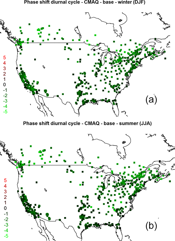
Phase shift of the diurnal cycle (in hours). A positive phase shift indicates that the model peak is “late”, while a negative phase shift indicates that the modelled peak precedes the observed peak. This analysis includes urban and suburban stations in addition to rural stations.

To perform this analysis, the modelled and observed ozone time series are first filtered to isolate the diurnal component using a KZ filter. Then, the cross covariance between the two time series is calculated. The time at which the maximum covariance value occurs is taken as the phase shift between the two signals. The method has an error of ±0.5 h.

In NA, the modelled diurnal peak occurs 1–2 h earlier than the observed diurnal peak at many stations and up to 3–4 h earlier at some Canadian stations. By taking into consideration the 0.5 h error of the estimate, the receptors at the western border (approximately corresponding to NA3) are least affected by this timing error (especially in summer Fig. 24b), and therefore the covariance share of the error shown in Fig. 4 is not due to daily phase shift in this region but probably due to the shifting of longer (or shorter) time periods induced for example by errors in transport (wind speed and/or direction). Figure S13 in the Supplement reports the same analysis repeated for the “zero emi” and “zero BC” runs.

In the EU (Fig. 25), no phase shift (or a phase shift compatible with the 0.5 h estimation error) is observed in Romania, Germany, or the UK during winter, while a significant phase shift (the modelled peak occurs upto6h early) is observed in the north of Italy and Austria, with France and Spain oscillating between positive 3 (model delay upto5h in the south of Madrid) and negative 5 and 6 h phase shifts, with the net effect of a spatially aggregated daily cycle that is in phase with the observations (Fig. 3b). During summer the phase shift is larger and extends also to the countries where the phase shift was null during winter. Moreover, some country-wise grouping can be detected, as for example at the border between Belgium and France, Spain and France, and Finland to Sweden, possibly due to the different measurement techniques and protocols among EU countries (e.g. Solazzo and Galmarini, 2015). Figure S14 in the Supplement reports the same analysis repeated for the “zero emi” run. The difference between the time shift of the base case and the zeroed emission scenario (Fig. S15) reveals the effects of the timing of the anthropogenic emissions on the covariance error. The effect is null over EU (median value of the difference of zero) and is very limited in NA (median value of zero during summer and of —1 during winter), reinforcing the conclusion that the timing of the emissions is not responsible for (or contributes very little to) the daily error.

Figure 25.

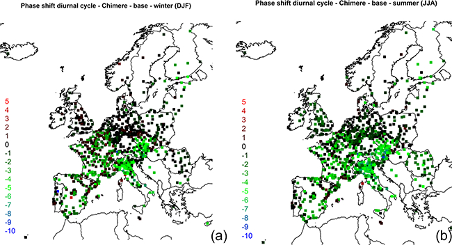
As in Fig. 24 for EU.

While errors in emission profiles obviously can be one cause of the phase shift and thus the covariance error of the modelled ozone signal, the representation of boundary layer processes clearly can be a factor as well. As discussed in e.g. Herwehe et al. (2011), the parameterisation of vertical mixing during transitional periods of the day can cause a time shift in the modelled ozone concentrations due to its effects on the near-surface concentrations of NO_x and ozone, which in turn affect the chemical regime and balance between ozone formation and removal.

To quantify the importance of the covariance error caused by a phase shift relative to other sources of error, Fig. 26 shows the curves of normalised MSE as the observed ozone time series is shifted with respect to itself between −10 and 10 h. The MSE curve equals zero for a zero-hour lag and is symmetric with respect to the sign of the lag. Since this analysis compares the observed signal to itself (with varying degrees of time lags), the MSE fraction of bias and variance is zero while all of the MSE is due to the covariance.

Figure 26.

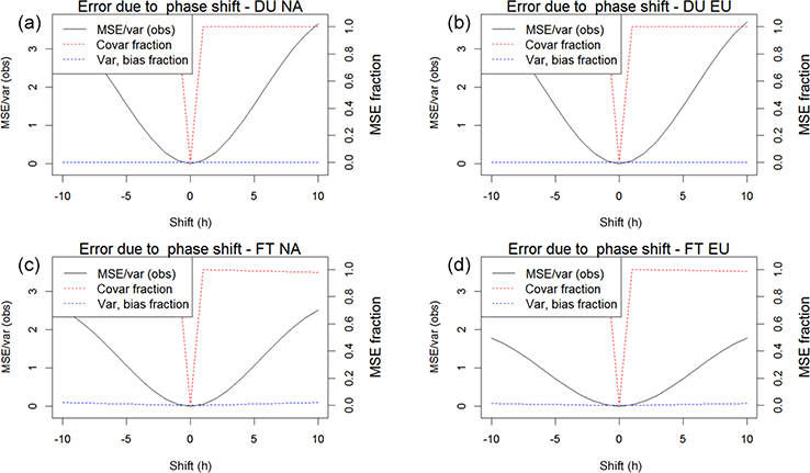
Normalised MSE produced by lagging the observed diurnal cycle with respect to itself. The MSE due to such a shift is entirely due to covariance error. The plots are presented for EU2 (b, d) and NA2 (a, c) for the months of JJA. Panels (a, b) shows the impact of the phase shift on the DU component, and (c, d) show results for the undecomposed time series (FT). For EU2, a shift of ±3 h causes an MSE of ~ 0.5 times the variance of the observations

The curves in Fig. 26 shows that a phase lag in the diurnal cycle of ±6 h causes a MSE error in the diurnal component of magnitude ~var(obs) (in both EU and NA), where var(obs) is the variance of the measured diurnal cycle (top panel). The effect on the full (undecomposed) time series is that a phase lag of ±4 (EU) and ±5–6 (NA) hour in the diurnal cycle causes a MSE error of magnitude ~var(obs), where in this case the variance is that of the undecomposed time series of ozone (lower panel).

Therefore, a modelled ozone peak that occurs 4 to 5 h too early (a feature that is detected at some EU3 and Canadian stations) corresponds to a covariance error of 9.0ppb (i.e. the standard deviation of the network-average ozone observations in summer in both EU and NA). This result also helps explain the large covariance error in EU3, which can be at least partially attributed to the large phase shift of the daily cycle.

4.4. Explaining the error of ozone

In this section a simple linear regression model for the error of ozone ΔO₃ is applied with the goal of detecting the causes of model errors on the daily and longer-term scales identified in the previous section. Although a linear model is overly simplistic and other methods are available (e.g kernel smoothers), we employed the simpler approach (i) since it is not the aim of this study to build a statistically accurate model for the model error and (ii) by pursuing simple reasoning we hope to identify the timescale of the error and the most likely fields causing it at that timescale. More advanced techniques are likely to overcomplicate the results and their interpretations but could be pursued in future studies.

The available regressors (explanatory variables) are the errors of the variables for which measurements have been collected within AQMEII, i.e. NO (EU only), NO₂, Temp, and WS:

$$\Delta {\mathrm{O}}_3={\beta }_1\Delta \mathrm{NO}+{\beta }_2\Delta {\mathrm{NO}}_2+{\beta }_3\Delta \mathrm{Temp}+{\beta }_4\Delta \mathrm{WS}+k,$$ (3)

where β_i are the coefficients of the multiple linear regression, and the intercept k is the portion of the ozone error not explainable by any of the regressors. A bootstrap analysis (Mudelsee, 2014; Groemping, 2006) is used to calculate the relative importance of each error field in explaining the variance of ΔO₃ (Figs. 27 and 28) with an uncertainty of ~5 %. The analysis is restricted to stations of ozone, NO_x, WS, and Temp that are located within a maximum horizontal distance of 1000 m and maximum vertical displacement of 250 m, to avoid error due to spatial heterogeneity. The number of stations is 61 in EU and 45 in NA.

Figure 27.

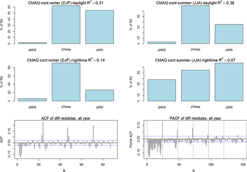
Percentage of variance explained by the regressors (the total R2 for the regression is reported in the title of each panel). The relative importance of each variable is assessed by using a bootstrap resampling. The plots at the bottom show the ACF and PACF of the yearly time series of residual of the fit, i.e. the portion of the ozone time series that was not captured by the linear regressions on the available variables. The analysis encompasses 47 co-located stations (the NA stations for ozone, NO2, WS, and Temp that fall in a radius of 1000 m and vertical displacement less than 250 m).

Figure 28.

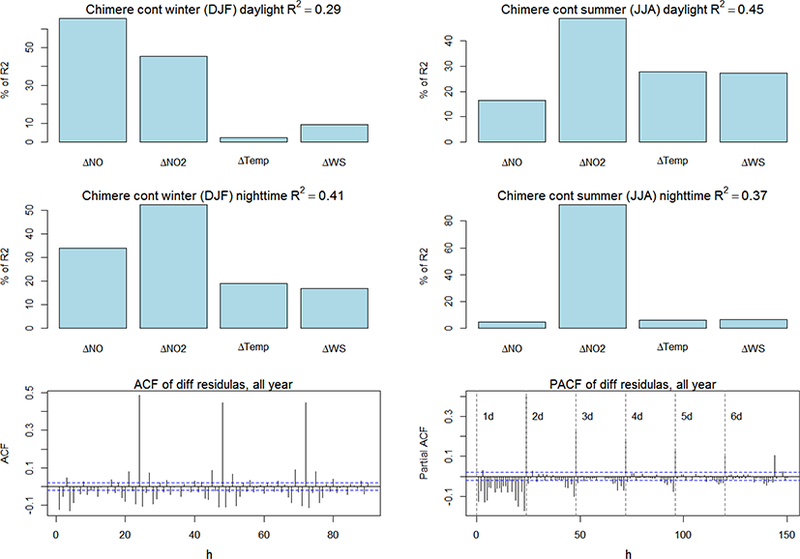
Same as Fig. 27 for EU. The analysis encompasses 61 co-located stations (the EU stations for ozone, NO, NO2, WS, and Temp that fall in a radius of 1000 m and vertical displacement less than 250 m).

The errors of temperature and wind speed explain about a third of the daylight winter ozone error of CMAQ, while ~20 % of the ozone error variability during daylight summer ozone is associated with the error in temperature and, to a lesser extent, wind speed (Fig. 27). In contrast, in Chimere the NO and NO2 error over EU during winter is correlated with the error of ozone, especially during nighttime (Fig. 28). Overall, there is no instance where the variance explained by the available variables (quantified through the coefficient of determination R²) exceeds 0.45 (corresponding to a linear correlation coefficient of ~0.67). The ACFs of the residuals of the regression show that there is an overwhelming daily memory of the error that can only partially be attributed to errors of the available regressor variables, pointing to the need to include additional variables in future applications of this regression analysis.

A straightforward limitation of Eq. (3) is that it assumes that successive values of the error terms are independent, while in practice this is not the case. Table 2 reports the correlation coefficient of the diurnal fluctuations of the residuals, obtained by filtering out fluctuations faster than ~1.5 days from the measured and observed time series (for the analysis of Table 2 the co-location restriction on the rural receptors is removed to allow spatial considerations, the only constraint is on the the vertical displacement among stations to be less than 250 m). Several significant collinearities can be detected (e.g between ΔWS and ATemp and between ΔNO₂ and ATemp, especially in winter).

Table 2.

Linear correlation coefficient between the diurnal residuals of the regressors of Eq. (3). The residuals are calculated by removing fluctuations faster the ~1.5 days from the measured and modelled time series. All the correlation values are significant up to 1 % significance threshold. (a) NA; (b) EU. For each set of variables, the regression analysis includes the rural stations within a maximum differential altitude of 250 m.

(a)	Correlation among diurnal components of residuals
	ΔNO2			ΔTemp			ΔWS
	NA1	NA2	NA3	NA1	NA2	NA3	NA1	NA2	NA3
SUMMER
ΔNO2	1	1	1	−0.6	−0.23	−0.65	−0.19	0.46	−0.26
ΔTemp	−0.6	−0.23	−0.65	1	1	1	0.62	0.53	0.7
ΔWS	−0.19	0.46	−0.26	0.62	0.53	0.7	1	1	1
WINTER
ΔNO2	1	1	1	−0.63	−0.57	−0.56	−0.55	−0.05	−0.19
ΔTemp	−0.63	−0.57	−0.56	1	1	1	−0.63	−0.47	−0.35
ΔWS	−0.55	−0.05	−0.19	0.49	0.47	0.35	1	1	1

(b)	Correlation among diurnal components of residuals
	ΔNO			ΔNO2			ΔTemp			ΔWS
	EU1	EU2	EU3	EU1	EU2	EU3	EU1	EU2	EU3	EU1	EU2	EU3
SUMMER
ΔNO	1	1	1	0.05	0.68	0.48	−0.08	−0.05	−0.27	−0.07	0.11	−0.02
ΔNO2	0.05	0.68	0.48	1	1	1	0.57	0.18	−0.27	0.51	0.38	0.26
ΔTemp	−0.08	−0.05	−0.27	0.57	0.18	−0.27	1	1	1	0.81	0.63	0.21
ΔWS	−0.07	0.11	−0.02	0.51	0.38	0.26	0.81	0.63	0.21	1	1	1
WINTER
ΔNO	1	1	1	0.31	0.6	0.73	0.02	−0.52	−0.62	0.03	0.12	0.06
ΔNO2	0.31	0.6	0.73	1	1	1	−0.13	−0.7	−0.7	−0.01	0.09	0.11
ΔTemp	0.02	−0.52	−0.62	−0.13	−0.7	−0.7	1	1	1	0.48	0.02	−0.01
ΔWS	0.03	0.12	0.06	−0.01	0.09	0.11	0.48	0.02	0.01	1	1	1

In addition to the collinearity issue, there are other endogenous variables that are not part of the regression analysis but whose error contributes to total ΔO₃, as revealed by the ACFs and PACFs of the first-order differentiated residuals of the regression, reported in the last panels of each plot. Such missing variables are likely to correlate with both the dependent (AO3) and the explanatory variables. For instance, errors in the cloud cover and/or radiation scheme, land use masking, etc. are shared by the chemical species (ozone and its precursors) as well as by the meteorological fields. The ACFs and PACFs suggest that the common omitted error of the fit propagates with daily recurrence and is not explained by the available variables, stressing the findings of the previous section and again pointing to PBL-related errors.

However, since we are not in a position to estimate the errors associated with PBL variables (radiation, temperature, turbulence), an alternate approach is to filter out the diurnal process from the modelled and observed time series and repeat the analysis based on Eq. (3) (Figs. S16 and S17). The correlation coefficients of the residuals with the diurnal component filtered out are reported in Table 3. The collinearity has been largely removed, especially for NA, while for EU some strong correlation persists (ΔNO₂ and ANO, and between ΔWS and ΔTemp in winter).

Table 3.

Linear correlation coefficient between the residuals of the regressors of Eq. (3), when the diurnal fluctuations are filtered out. The residuals are calculated by removing fluctuations faster the ~1.5 days. All the correlation values are significant up to 1 % significance threshold from the measured and modelled time series. (a) NA; (b) EU. For each set of variables, the regression analysis includes the rural stations within a maximum differential altitude of 250 m.

(a)	Correlation among residuals (diurnal fluctuations removed)
	ΔNO2			ΔTemp			ΔWS
	NA1	NA2	NA3	NA1	NA2	NA3	NA1	NA2	NA3
SUMMER
ΔNO2	1	1	1	−0.2	−0.02	−0.26	−0.06	−0.05	−0.19
ΔTemp	−0.2	−0.02	−0.26	1	1	0.28	0.09	0.42
ΔWS	−0.06	−0.05	−0.19	0.28	0.09	0.42	1	1	1
WINTER
ΔNO2	1	1	1	−0.12	−0.42	−0.03	−0.02	−0.16	−0.11
ΔTemp	−0.12	−0.42	−0.03	1	1	1	0.54	0.34	0.13
ΔWS	−0.02	−0.16	−0.11	0.54	0.34	0.13	1	1	1

(b)	Correlation among residuals (diurnal fluctuations removed)
	ΔNO			ΔNO2			ΔTemp			ΔWS
	EU1	EU2	EU3	EU1	EU2	EU3	EU1	EU2	EU3	EU1	EU2	EU3
SUMMER
ΔNO	1	1	1	0.22	0.71	0.69	0.12	−0.23	−0.03	0.06	−0.23	−0.08
ΔNO2	0.22	0.71	0.69	1	1	1	−0.27	−0.41	−0.11	0.54	−0.43	−0.01
ΔTemp	0.12	−0.23	−0.03	−0.27	−0.41	−0.11	1	1	1	0.44	0.22	0.36
ΔWS	0.06	−0.23	−0.08	−0.54	−0.43	−0.01	0.44	0.22	0.36	1	1	1
WINTER
ΔNO	1	1	1	0.21	0.64	0.46	−0.22	−0.19	−0.02	−0.15	−0.14	−0.01
ΔNO2	0.21	0.64	0.46	1	1	1	−0.09	−0.38	−0.35	−0.07	−0.2	−0.08
ΔTemp	−0.22	−0.19	−0.02	−0.09	−0.38	−0.35	1	1	1	0.37	−0.1	0.38
ΔWS	−0.15	−0.14	−0.01	−0.07	−0.2	−0.08	0.37	−0.1	0.38	1	1	1

The R² of the regression for the “no-DU” case drops drastically in NA, while keeping approximately the same values in EU (but in EU3 R² does not exceed 0.10; not shown) as shown in Figs. S16 and S17. Moreover, this analysis and its comparison to the results presented in earlier sections lead to the following conclusions:

• –A strong daily error component is common to all variables investigated here.
• –This error manifests itself in the correlation coefficient and thus is due to a variance/covariance type of error (otherwise, if it was a bias-type error, the R² would have been similar between the analysis of the signal with and without the diurnal component).
• –By inspecting the “no-DU” case, at least in NA (Fig. S16), the bias error discussed in Sect. 3 cannot be explained simply in terms of the fields NO₂, Temp, and WS. Hence, the bias of the CMAQ model over the NA continent appears to be associated with processes with longer timescales (i.e. longer than daily), such as boundary conditions (inducing mostly bias error, as discussed in Sect. 3), deposition, and/or transport (potential systematic errors in wind direction, for example, would likely produce a bias-type error).
• –The impact of ANO₂ and ANO in EU (all subregions, mostly daylight) and of AWS in EU1 (and partially EU2) on the error of ozone (not shown) is similar with and without the diurnal fluctuations, indicating cross correlation of these error fields for periods longer than 1 day.

5. Discussions

The application of several diagnostic techniques in conjunction with sensitivity scenarios has allowed in-depth analysis of the timescale properties of the ozone error of CMAQ and Chimere, two widely applied modelling systems. The main results, as stemming from various aspects of the investigation, are that the largest share of MSE (~70–85 %) is associated with fluctuations longer than the daily scale and mostly due to offsetting error in NA and due to covariance error in EU, while the remaining MSE is due to processes with daily variation. The causes of the long-term error need to be sought in the fields that produce (mainly) a bias type of error such as emissions, boundary conditions, and deposition for NA, while the time shift of the slow fluctuations in EU is possibly due to timing error of the synoptic drivers or other synoptic processes.

By excluding other plausible causes, and assuming that observational data are “correct” (not affected by systematic errors), we can conclude based on multiple indicators that the dynamics of the boundary layer (which in turn depend on the representation of radiation, surface characteristics, surface energy balance, heat exchange processes, development or suppression of convection, shear generated turbulence, and entrainment and detrainment processes at the boundary layer top for heat and any other scalars) are responsible for the recursive daily error. The most revealing indicator is the analysis of the ACF and PACF of the time series of ozone residuals that shows a daily periodicity: the 24 h errors are highly associated throughout the year; i.e. the error repeats itself with daily regularity. This could be caused by multiple processes occurring on a daily timescale, such as chemical transformations, the timing of the emissions, and PBL dynamics. However, analyses of the error periodicity of primary species (to exclude the role of chemical transformations) and of the scenario with zeroed anthropogenic emissions (to exclude the role of emissions) have shown the same error structure, pointing to PBL processes as the main cause of daily error.

Due to the spatial aggregation of these analyses and the non-linearity of the models’ components, it is possible that the periodicity of the error could be due to a combination of multiple processes at specific sites. However, the absence of a spatial or emission dependence and the persistence of the daily periodicity indicate that the main cause of the daily error stems from PBL dynamics. Furthermore, the analogies of the time shift of the diurnal component of the base and zeroed emission cases suggest that the timing error (pure covariance error) is not caused by anthropogenic emissions (with the possible exception of winter in NA where some small differences are present).

6. Conclusions

This study is part of the goal of AQMEII to promote innovative insights into the evaluation of regional air quality models. This study is primarily meant to introduce evaluation methods that are innovative and that move towards diagnosing the causes of model error. It focuses on the diagnostic of the error produced by CMAQ and Chimere applied to calculate hourly surface ozone mixing ratios over North America and Europe.

We argue that the current widespread practice (although with several exceptions) of using time-aggregate metrics to merely quantify the average distance (in a metric space) between models and observations has clear limitations and does not help target the causes of model error. We therefore propose to move towards the qualification of the error components (bias, variance, covariance) and to assess each of them with relevant diagnostic methods. At the core of the diagnostic methods we have devised over the years within AQMEII is the quality of the information that can be extracted from model and measurements to aid understanding of the causes of model error, thus providing more useful information to model developers and users than can be gained from aggregate metrics. Applying such approaches on a routine basis would help boost the confidence in using models prediction for various applications. At the current stage, the methods we propose help identify the timescale of the error and its periodicity. The step to link the error to specific processes can only be reached by integrating the analysis with sensitivity model runs. For instance, we can infer that the timing error of the diurnal component is (at least partially) associated with the dynamics of the PBL, but further analyses are necessary to isolate the components of the PBL responsible for that error.

While remarking that the analyses carried out are not meant to compare the two models but are rather meant to show how the two models, applied to different areas and using different emissions, respond to changes, the main conclusions of this study are as follows:

• –While the zeroing/modification of input of ozone from the lateral boundaries causes a shift of the ozone diurnal cycle in both CMAQ and Chimere, the response of the two models to a modification of anthropogenic emission and deposition fluxes is very different. For CMAQ, the effect of removing anthropogenic emissions causes a shift and a flattening of the diurnal curve (bias and variance error), while for Chimere the effect is restricted to a shift. In contrast, setting the ozone dry deposition velocity to zero causes a shift (bias error) for CMAQ, while a profound change of the error structure occurs for Chimere with significant impacts on not only the bias but also the variance and covariance terms.
• –The response of the models to variations in anthropogenic emissions and boundary conditions show a pronounced spatial heterogeneity, while the seasonal variability of this response is found to be less marked. Only during the winter season does the zeroing of boundary values for North America produce a spatially uniform deterioration of the model accuracy across the majority of the continent.
• –Fluctuations slower than ~1.5 days account for 70–85% of the total ozone quadratic error. The partition of this error into bias, variance, and covariance depends on season and region. In general, the CMAQ model suffers mostly from bias error (model overestimation during summer and underestimation during winter), while the Chimere model is rather “centred” (i.e. almost unbiased) but suffers high covariance error (associated with the timing of the signal and thus likely to synoptic drivers).
• –A recursive, systematic error with daily periodicity is detected in both models, responsible for 10–20 % of the quadratic total error, possibly associated with the dynamics of the PBL.
• –The modelled ozone daily peak accurately reproduces the observed one, although with significant exceptions in France, Italy, and Austria for Chimere and with the exceptions of Canada and some areas in the eastern US for CMAQ. Assuming the accurateness of the observational data in these regions, the modelled peak is anticipated by up to 6 h, causing a covariance error as large as 9ppb. The analysis suggests that the timing of the anthropogenic emissions is not responsible for the phasing error of the ozone peaks but rather indicates that it might be caused by the dynamics of the PBL (although the role of biogenic emissions and chemistry cannot be ruled out).
• –The ozone error in CMAQ has a weak/negligible dependence on the error of NO₂ and wind speed, while the error of NO₂ impacts significantly the ozone error produced by Chimere. On timescales longer than 1.5 days, the Chimere ozone error is significantly associated with the error of wind speed and temperature.

Although having exploited several evaluation frameworks over the past 10 years within AQMEII (operational, diagnostic, and probabilistic) the goal of clearly associating errors to processes has not yet been achieved. As already suggested in the conclusions of the collective analysis of the AQMEII3 suite of model runs summarised by Solazzo et al. (2017), future model evaluation activities would benefit from incorporating sensitivity simulations and process specific analyses that help to disentangle the non-linearity of the many model variables, possibly by focusing on smaller modelling communities. The “theory of evaluation” being put forward by the hydrology modelling community (Nearing et al., 2016, and references therein) may provide a template for the air quality community to further advance their model evaluation approaches.

Data availability.

The modeling and observational data generated for the AQMEII exercise are accessible through the ENSEMBLE data platform (http://ensemble.jrc.ec.europa.eu/) upon contact with the managing organizations. References to the repositories of the observational data used have been provided in Sect. 2.1.

Figure 8.

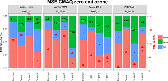
As in Fig. 6 for the hourly time series of “zeroed anthropogenic emissions” scenario.

Figure 9.

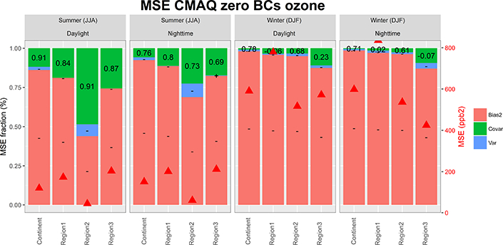
As in Fig. 6 for the hourly time series of the “zeroed boundary conditions” scenario.

Figure 12.

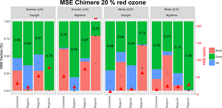
As in Fig. 11 for the hourly time series of “20 % reduction” scenario

Figure 13.

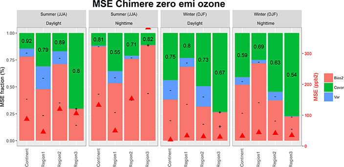
As in Fig. 11 for the hourly time series of “zeroed anthropogenic emissions” scenario.

Appendix A

The ACF is derived by the autocovariance (ACV) and expresses the correlation of a time series with its lagged version (e.g. Chatfield, 2004):

$$\begin{gathered} \text{ACV}(k)=E\left\{[X\left(t\right)-\mu ][X\left(t+k\right)-\mu ]\right\} \\ =\mathrm{Cov}\left[X\left(t\right)X\left(t+k\right)\right]; \\ \text{ACF}\left(k\right)=\text{ACV}\left(k\right)/\text{ACV}\left(0\right). \end{gathered}$$

At any lag k, the ACV coefficients c_k are given by

$$c_k=\frac{1}{N}{\displaystyle \sum _{t=1}^{N-k}(x_t-\overline{x})(x_{t+k}-\overline{x}).}$$

As usual, the autocorrelation coefficients are given by normalising c_k with c₀.

The PACF measures the excess of correlation between two elements of X(t) lagged by s elements not accounted for by the autocorrelation of the intermediate s-1 elements. In other words, the ACF of X(t) and X(t+s) includes all the linear dependence between the intermediate s - 1 lags. The PACF allows us to investigate the direct effect of lag t on the lag t +s.

The advantage of using ACFs and PACFs is that they are a function of the lag k only (and not of the specific time t). This condition holds only if X (t) is stationary (i.e. its mean and variance do not change over time). Several tests are available to check X (t) for stationarity (e.g. Chatfield, 2004). Differencing the time series is typically a way to achieve stationarity.

References

- Appel KW, Chemel C, Roselle SJ, Francis XV, Hu R-M, Sokhi RS, Rao ST, and Galmarini S: Examination of the Community Multiscale Air Quality (CMAQ) model performance for North America and Europe for the AQMEII project, Atmos. Environ, 53, 142–155, 2012. [Google Scholar]
- Appel KW, Napelenok SL, Foley KM, Pye HOT, Hogrefe C, Luecken DJ, Bash JO, Roselle SJ, Pleim JE, Foroutan H, Hutzell WT, Pouliot GA, Sarwar G, Fahey KM, Gantt B, Gilliam RC, Heath NK, Kang D, Mathur R, Schwede DB, Spero TL, Wong DC, and Young JO: Description and evaluation of the Community Multiscale Air Quality (CMAQ) modeling system version 5.1, Geosci. Model Dev, 10, 1703–1732, 10.5194/gmd-10-1703-2017, 2017. [DOI] [PMC free article] [PubMed] [Google Scholar]
- Atlas EL, Ridley BA, and Cantrell C: The Tropospheric Ozone Production about the Spring Equinox (TOPSE)Experiment: Introduction, J. Geophys. Res, 108, 8353, 10.1029/2002JD003172, 2003. [DOI] [Google Scholar]
- Bessagnet B, Pirovano G, Mircea M, Cuvelier C, Aulinger A, Calori G, Ciarelli G, Manders A, Stern R, Tsyro S, Garcia Vivanco M, Thunis P, Pay M-T, Colette A, Couvidat F, Meleux F, Rouil L, Ung A, Aksoyoglu S, Baldasano JM, Bieser J, Briganti G, Cappelletti A, D’Isidoro M, Fi-nardi S, Kranenburg R, Silibello C, Carnevale C, Aas W, Dupont J-C, Fagerli H, Gonzalez L, Menut L, Prévôt ASH, Roberts P, and White L: Presentation of the EURODELTA III intercomparison exercise - evaluation of the chemistry transport models’ performance on criteria pollutants and joint analysis with meteorology, Atmos. Chem. Phys, 16, 12667–12701, 10.5194/acp-16-12667-2016, 2016. [DOI] [Google Scholar]
- Bonasoni P, Evangelisti F, Bonafe U, Ravegnani F, Calzolari F, Stohl A, Tositti L, Tubertini O, and Colombo T: Stratospheric ozone intrusion episodes recorded at Mt. Cimone during the VOLTALP project: case studies, Atmos. Environ, 34, 1355–1365, 2000. [Google Scholar]
- Byun DW and Schere KL: Review of the governing equations, computational algorithms, and other components of the Models-3 community Multiscale Air Quality (CMAQ) modelling system, Appl. Mech. Rev, 59, 51–77, 2006. [Google Scholar]
- Camalier L, Cox W, and Dolwick P: The effects of meteorology on ozone in urban areas and their use in assessing ozone trends, Atmos. Environ, 41, 7127–7137, 10.1016/j.atmosenv.2007.04.061, 2007. [DOI] [Google Scholar]
- Chatfield C: The analysis of time series An introducton, 6th Edn., Chapman & Hall/CRC, 2004. [Google Scholar]
- Dennis R, Fox T, Fuentes M, Gilliland A, Hanna S, Hogrefe C, Irwin J, Rao ST, Scheffe R, Schere K, Steyn D, and Venkatram A: A framework for evaluating regional-scale numerical photochemical modelling systems, Environ. Fluid Mech, 10, 471–489, 2010. [DOI] [PMC free article] [PubMed] [Google Scholar]
- Enthekabi D, Reichle RH, Koster RD, and Crow WT: Performance metrics for soil moisture retrievals and application requirements, J. Hydrometeorol, 11, 832–840, 2010. [Google Scholar]
- Galmarini S, Kioutsioukis I, and Solazzo E: Epluribus unum*: ensemble air quality predictions, Atmos. Chem. Phys, 13, 7153–7182, 10.5194/acp-13-7153-2013, 2013. [DOI] [Google Scholar]
- Galmarini S, Koffi B, Solazzo E, Keating T, Hogrefe C, Schulz M, Benedictow A, Griesfeller JJ, Janssens-Maenhout G, Carmichael G, Fu J, and Dentener F: Technical note: Coordination and harmonization of the multi-scale, multi-model activities HTAP2, AQMEII3, and MICS-Asia3: simulations, emission inventories, boundary conditions, and model output formats, Atmos. Chem. Phys, 17, 1543–1555, 10.5194/acp-17-1543-2017, 2017. [DOI] [PMC free article] [PubMed] [Google Scholar]
- Groemping U: Relative Importance for Linear Regression in R: The Package relaimpo, J. Stat. Softw, 17, 1–27, 2006. [Google Scholar]
- Guenther AB, Jiang X, Heald CL, Sakulyanontvittaya T, Duhl T, Emmons LK, and Wang X: The Model of Emissions of Gases and Aerosols from Nature version 2.1 (MEGAN2.1): an extended and updated framework for modeling biogenic emissions, Geosci. Model Dev, 5, 1471–1492, 10.5194/gmd-5-1471-2012, 2012. [DOI] [Google Scholar]
- Gupta HV, Wagener T, and Liu Y: Reconciling theory with observations: elements of a diagnostic approach to model evaluation, Hydrol. Process, 22, 3802–3813, 2008. [Google Scholar]
- Gupta HV, Kling H, Yilamz KK, and Martinez GF: Decomposition of the mean sqaure error and NSE perforamnce criteria: implications for improving hydrological modelling, J. Hydrol, 377, 80–91, 2009. [Google Scholar]
- Herwehe JA, Otte TL, Mathur R, and Rao ST: Diagnostic analysis of ozon concentrations simulated by two regional-scale air quality models, Atmos. Environ, 45, 5957–5969, 2011. [Google Scholar]
- Hogrefe C, Rao ST, Zurbenko IG, and Porter PS: Interpreting the information in ozone observations and model predictions relevant to regulatory policies in the Eastern United States, B. Am. Meteorol. Soc, 81, 2083–2106, 2000. [Google Scholar]
- Hogrefe C, Roselle S, Mathur R, Rao ST, and Galmarini S: Space-time analysis of the Air Quality Model Evaluation International Initiative (AQMEII) Phase 1 air quality simulations, J. Air Waste Manage, 64, 388–405, 2014. [DOI] [PubMed] [Google Scholar]
- Im U, Bianconi R, Solazzo E, Kioutsioukis I, Badia A, Balzarini A, Baro R, Bellasio R, Brunner D, Chemel C, Curci G, Denier van der Gon H, Flemming J, Forkel R,Giordano L, Jimenez-Guerrero P, Hirtl M, Hodzic A, Honzak L, Jorba O, Knote C, Makar PA, Manders-Groot A, Neal L, Pdrez JL, Pirovano G, Pouliot G, San Jose R, Savage N, Schroder W, Sokhi RS, Syrakov D, Torian A, Tuccella P, Wang K, Werhahn J, Wolke R, Zabkar R, Zhang Y, Zhang J, Hogrefe C, and Galmarini S: Evaluation of operational online coupled regional air quality models over Europe and North America in the context of AQMEII phase 2. Part II: particulate matter, Atmos. Environ, 115, 421–441, 2015a. [Google Scholar]
- Im U, Bianconi R, Solazzo E, Kioutsioukis I, Badia A, Balzarini A, Baro R, Bellasio R, Brunner D, Chemel C, Curci G, Flemming J, Forkel R, Giordano L, Jimenez-Guerrero P, Hirtl M, Hodzic A, Honzak L, Jorba O, Knote C, Kuenen JJP, Makar PA, Manders-Groot A, Neal L, Pdrez JL, Pirovano G, Pouliot G, San Jose R, Savage N, Schroder W, Sokhi RS, Syrakov D, Torian A, Tuccella P, Werhahn J, Wolke R, Yahya K, Zabkar R, Zhang Y, Zhang J, Hogrefe C, and Galmarini S: Evaluation of operational online-coupled regional air quality models over Europe and North America in the context of AQMEII phase 2. Part I: ozone, Atmos. Environ, 115, 404–420, 2015b. [Google Scholar]
- Kioutsioukis I, Im U, Solazzo E, Bianconi R, Badia A, Balzarini A, Baró R, Bellasio R, Brunner D, Chemel C, Curci G, van der Gon HD, Flemming J, Forkel R, Giordano L, Jiménez-Guerrero P, Hirtl M, Jorba O, Manders-Groot A, Neal L, Pérez JL, Pirovano G, San Jose R, Savage N, Schroder W, Sokhi RS, Syrakov D, Tuccella P, Werhahn J, Wolke R, Hogrefe C, and Galmarini S: Insights into the deterministic skill of air quality ensembles from the analysis of AQMEII data, Atmos. Chem. Phys, 16, 15629–15652, 10.5194/acp-16-15629-2016, 2016. [DOI] [Google Scholar]
- Lattuati M: Impact des emissions européennes sur le bilan d’ozone troposphérique à l’interface de l’Europe et de l’Atlantique Nord: apport de la modélisation lagrangienne et des mesures en altitude, PhD Thesis, Universitd Pierre et Marie Curie, Paris, France, 1997. [Google Scholar]
- Lemaire VEP, Colette A, and Menut L: Using statistical models to explore ensemble uncertainty in climate impact studies: the example of air pollution in Europe, Atmos. Chem. Phys, 16, 2559–2574, 10.5194/acp-16-2559-2016, 2016. [DOI] [Google Scholar]
- Logan JA: An analysis of ozonesonde data for the troposphere: Recom-mendations for testing 3-D models and development of a gridded climatology for tropospheric ozone, J. Geophys. Res, 104, 16115–16149, 1999. [Google Scholar]
- Makar PA, Gong W, Mooney C, Zhang J, Davignon D, Samaali M, Moran MD, He H, Tarasick DW, Sills D, and Chen J: Dynamic adjustment of climatological ozone boundary conditions for air-quality forecasts, Atmos. Chem. Phys, 10, 8997–9015, 10.5194/acp-10-8997-2010, 2010. [DOI] [Google Scholar]
- Makar PA, Staebler RM, Akingunola A, Zhang J, McLinden C, Kharol SK, Pabla B, Cheung P, and Zheng Q: The effects of forest canopy shading and turbulence on boundary layer ozone, Nat. Commun, 8, 15243, 10.1038/ncomms15243, 2017. [DOI] [PMC free article] [PubMed] [Google Scholar]
- Menut L, Bessagnet B, Khvorostyanov D, Beekmann M, Blond N, Colette A, Coll I, Curci G, Foret G, Hodzic A, Mailler S, Meleux F, Monge J-L, Pison I, Siour G, Turquety S, Valari M, Vautard R, and Vivanco MG: CHIMERE 2013: a model for regional atmospheric composition modelling, Geosci. Model Dev, 6, 981–1028, 10.5194/gmd-6-981-2013, 2013. [DOI] [Google Scholar]
- Mudelsee M: Climate time series analysis, 2nd Edn., Springer, Switzerland, 2014. [Google Scholar]
- Murphy AH: Skill scores based on the mean square error and their relationships to the correaltion coefficient, Mon. Weather Rev, 116, 2417–2424, 1988. [Google Scholar]
- Murphy AH: What is a good forecast?: An essay on the nature of goodness in weather forecasting, Weather Forecast., 8, 281–293, 1993. [Google Scholar]
- Murphy AH: The coefficient of correlation and determination as measures of performance in forecast verification, Weather Forecast., 10, 681–688, 1995. [Google Scholar]
- Otero N, Sillmann J, Schnell JL, Rust HW, and Butler T: Synoptic and meteorological divers of extreme ozone concentrations over Europe, Environ. Res. Lett, 11, 024005, 10.1088/1748-9326/11/2/024005, 2016. [DOI] [Google Scholar]
- Penkett SA and Brice KA: The spring maximum in photooxidants inthe Northern Hemisphere troposphere, Nature, 319, 655–657, 1986. [Google Scholar]
- Pleim J and Ran L: Surface Flux Modeling for Air Quality Applications, Atmosphere, 2, 271–302, 2011. [Google Scholar]
- Potempski S and Galmarini S: Est modus in rebus: analytical properties of multi-model ensembles, Atmos. Chem. Phys, 9, 9471–9489, 10.5194/acp-9-9471-2009, 2009. [DOI] [Google Scholar]
- Nearing GS, Tian Y, Gupta HV, Clark MP, Harrison KW, and Wejs V: A philosophical basis for hydrological uncertainty, Hydrolog. Sci. J, 6, 1666–1678, 2016. [Google Scholar]
- Rao ST, Galmarini S, and Puckett K: Air quality model evaluation international initiative (AQMEII), B. Am. Meteorol. Soc, 92, 23–30, 10.1175/2010BAMS3069.1, 2011. [DOI] [Google Scholar]
- Simon H, Baker KR, and Phillips S: Compilation and interpretation of photochemical mpdel performance statistics published between 2006 and 2012, Atmos. Environ, 61, 124–139, 2012. [Google Scholar]
- Skamarock WC, Klemp JB, Dudhia J, Gill DO, Barker DM, Duda MG, Huang X-Y, Wang W, and Powers JG: A description of the advanced research WRF version 3, NCAR Tech Note NCAR/TN 475 STR, 125 pp., 2008. [Google Scholar]
- Solazzo E and Galmarini S: Comparing apples with apples: Using spatially distributed time series of monitoring data for model evaluation, Atmos. Environ, 112, 234–245, 2015. [Google Scholar]
- Solazzo E and Galmarini S: Error apportionment for atmospheric chemistry-transport models - a new approach to model evaluation, Atmos. Chem. Phys, 16, 6263–6283, 10.5194/acp-16-6263-2016, 2016. [DOI] [Google Scholar]
- Solazzo E, Bianconi R, Vautard R, Appel KW, Moran MD, Hogrefe C, Bessagnet B, Brandt J, Christensen JH, Chemel C, Coll I, van der Gon HD, Ferreira J, Forkel R, Francis XV, Grell G, Grossi P, Hansen AB, Jerice-vic A, Kraljevic L, Miranda AI, Nopmongcol U, Pirovano G, Prank M, Riccio A, Sartelet KN, Schaap M, Silver JD, Sokhi RS, Vira J, Werhahn J, Wolke R, Yarwood G, Zhang J, Rao ST, and Galmarini S: Model evaluation and ensemble modelling of surface-level ozone in Europe and North America in the context of AQMEII, Atmos. Environ, 53, 60–74, 2012a. [Google Scholar]
- Solazzo E, Bianconi R, Pirovano G, Matthias V, Vautard R, Moran MD, Appel KW, Bessagnet B, Brandt J, Christensen JH, Chemel C, Coll I, Ferreira J, Forkel R, Francis XV, Grell G, Grossi P, Hansen AB, Hogrefe C, Miranda AI, Nopmongco U, Prank M, Sartelet KN, Schaap M, Silver JD, Sokhi RS, Vira J, Werhahn J, Wolke R, Yarwood G, Zhang J, Rao ST, and Galmarini S: Operational model evaluation for particulate matter in Europe and North America in the context of AQMEII, Atmos. Environ, 53, 75–92, 2012b. [Google Scholar]
- Solazzo E, Bianconi R, Pirovano G, Moran MD, Vautard R, Hogrefe C, Appel KW, Matthias V, Grossi P, Bessagnet B, Brandt J, Chemel C, Christensen JH, Forkel R, Francis XV, Hansen AB, McKeen S, Nopmongcol U, Prank M, Sartelet KN, Segers A, Silver JD, Yarwood G, Werhahn J, Zhang J, Rao ST, and Galmarini S: Evaluating the capability of regional-scale air quality models to capture the vertical distribution of pollutants, Geosci. Model Dev, 6, 791–818, 10.5194/gmd-6-791-2013, 2013. [DOI] [Google Scholar]
- Solazzo E, Bianconi R, Hogrefe C, Curci G, Tuccella P, Alyuz U, Balzarini A, Bard R, Bellasio R, Bieser J, Brandt J, Christensen JH, Colette A, Francis X, Fraser A, Vi-vanco MG, Jimdnez-Guerrero P, Im U, Manders A, Nopmongcol U, Kitwiroon N, Pirovano G, Pozzoli L, Prank M, Sokhi RS, Unal A, Yarwood G, and Galmarini S: Evaluation and error apportionment of an ensemble of atmospheric chemistry transport modeling systems: multivariable temporal and spatial breakdown, Atmos. Chem. Phys, 17, 3001–3054, 10.5194/acp-17-3001-2017, 2017. [DOI] [PMC free article] [PubMed] [Google Scholar]
- Theil H: Economic forecast and policy, North-Holland pub., Amsterdam, 1961. [Google Scholar]
- Tian Y, Nearing GS, Peters-Lidard CD, Harrison KW, and Tang L: Performance metric, error modelling and uncertainty quantification, Am. Meteorol. Soc, 144, 607–613, 2016. [Google Scholar]
- Travis KR, Jacob DJ, Fisher JA, Kim PS, Marais EA, Zhu L, Yu K, Miller CC, Yantosca RM, Sulprizio MP, Thompson AM, Wennberg PO, Crounse JD, St. Clair JM, Cohen RC, Laughner JL, Dibb JE, Hall SR, Ullmann K, Wolfe GM, Pollack IB, Peischl J, Neuman JA, and Zhou X: Why do models overestimate surface ozone in the Southeast United States?, Atmos. Chem. Phys, 16, 13561–13577, 10.5194/acp-16-13561-2016, 2016. [DOI] [PMC free article] [PubMed] [Google Scholar]
- Torrence C and Compo GP: A Practical Guide to Wavelet Analysis, B. Am. Meteorol. Soc, 79, 61–78, 1997. [Google Scholar]
- Vautard R, Moran MD, Solazzo E, Gilliam RC, Matthias V, Bianconi R, Chemel C, Ferreira J, Geyer B, Hansen AB, Jericevic A, Prank M, Segers A, Silver JD, Werhahn J, Wolke R, Rao ST, and Galmarini S: Evaluation of the meteorological forcing used for the Air Quality Model Evaluation International Initiative (AQMEII) air quality simulations, Atmos. Environ, 53, 15–37, 2012. [Google Scholar]
- Wagener T and Gupta HV: Model identification for hydrological forecasting under uncertainty, Stochastic Enironmental Research, 19, 378–387, 2005. [Google Scholar]
- Weijs SV, Schoups G, and van de Giesen N: Why hydrological predictions should be evaluated using information theory, Hydrol. Earth Syst. Sci, 14, 2545–2558, 10.5194/hess-14-2545-2010, 2010. [DOI] [Google Scholar]
- Wesely ML: Parameterization of surface resistances to gaseous dry deposition in regional-scale numerical models, Atmos. Environ, 23, 1293–1304, 1989. [Google Scholar]
- Wilks DS: Statistical methods in atmospheric siences, Academic Press, Cambridge, Massachusetts, USA, 2011. [Google Scholar]
- Wilmott CJ: On the validation of models, Phys. Geogr, 2, 184194, 1981. [Google Scholar]
- Whitten GZ, Heo G, Kimura Y, McDonald-Buller E, Allen DT, Carter WPL, and Yarwood G: A new condensed toluene mechanism for Carbon Bond: CB05-TU, Atmos. Environ, 44, 5346–5355, 2010. [Google Scholar]
Associated Data
This section collects any data citations, data availability statements, or supplementary materials included in this article.
Supplementary Materials
Data Availability Statement