Evaluation and error apportionment of an ensemble of atmospheric chemistry transport modeling systems: multivariable temporal and spatial breakdown

Abstract

Through the comparison of several regional-scale chemistry transport modeling systems that simulate meteorology and air quality over the European and North American continents, this study aims at (i) apportioning error to the responsible processes using timescale analysis, (ii) helping to detect causes of model error, and (iii) identifying the processes and temporal scales most urgently requiring dedicated investigations.

The analysis is conducted within the framework of the third phase of the Air Quality Model Evaluation International Initiative (AQMEII) and tackles model performance gauging through measurement-to-model comparison, error decomposition, and time series analysis of the models biases for several fields (ozone, CO, SO₂, NO, NO₂, PM₁₀, PM_2.5, wind speed, and temperature). The operational metrics (magnitude of the error, sign of the bias, associativity) provide an overallsense of model strengths and deficiencies, while apportioning the error to its constituent parts (bias, variance, and covariance) can help assess the nature and quality of the error. Each of the error components is analyzed independently and apportioned to specific processes based on the corresponding timescale (long scale, synoptic, diurnal, and intraday) using the error apportionment technique devised in the former phases of AQMEII.

The application of the error apportionment method to the AQMEII Phase 3 simulations provides several key insights. In addition to reaffirming the strong impact of model inputs (emission and boundary conditions) and poor representation of the stable boundary layer on model bias, results also highlighted the high interdependencies among meteorological and chemical variables, as well as among their errors. This indicates that the evaluation of air quality model performance for individual pollutants needs to be supported by complementary analysis of meteorological fields and chemical precursors to provide results that are more insightful from a model development perspective. This will require evaluaion methods that are able to frame the impact on error of processes, conditions, and fluxes at the surface. For example, error due to emission and boundary conditions is dominant for primary species (CO, particulate matter (PM)), while errors due to meteorology and chemistry are most relevant to secondary species, such as ozone. Some further aspects emerged whose interpretation requires additional consideration, such as the uniformity of the synoptic error being region- and model-independent, observed for several pollutants; the source of unexplained variance for the diurnal component; and the type of error caused by deposition and at which scale.

1. Introduction

The Air Quality Model Evaluation International Initiative (AQMEII; Rao et al., 2011) has been active since 2008 with the aim of promoting research on regional air quality model evaluation across the modeling communities of Europe and North America. It is coordinated by the European Joint Research Centre (JRC) and the US Environmental Protection Agency (EPA) and it has now reached its third phase, referred to as AQMEII3 hereafter. The experience gathered in the first two phases consisted of important advancement in the model evaluation research as well as establishing a large community of participating regional modeling groups. This has made AQMEII a natural candidate for collaborating with the Hemispheric Transport of Air Pollutants (HTAP) initiative. HTAP, a task force of the Long Range Transport of Air Pollutants (LTRAP) program acting within the United Nations Economic Commission for Europe (UNECE) program, relies on a community of global-scale chemical transport models to investigate the fate of air pollutants emitted in the Northern Hemisphere and to determine the contribution of remote sources as well as their impacts on background concentration in different parts of the globe. HTAP is in its second phase and the activities undertaken during this second phase include coordinating simulations by both global- and regional-scale models. The regions of interest in the Northern Hemisphere are North America, Europe, and Southeast Asia. The regional-scale modeling component of this activity for Europe and North America is being coordinated by AQMEII, while the Asian component is being coordinated by MICs-ASIA (Model Intercomparison Study Asia). Global-scale models participating in HTAP are used by the AQMEII regional models as boundary conditions, and special attention has been given to the emission inventory to ensure that it is consistent between the global- and regional-scale simulations as described in Janssens-Maenhout et al. (2015). The activity described here relates to the evaluation of the base case scenario set up within the context of HTAP and AQMEII (Galmarini et al., 2017).

Following the simulation strategy developed over the first two phases of the AQMEII activity, two continental-scale domains were used in the exercise - one over Europe (EU) and one over North America (NA; Fig. 1). The modeling groups participating in AQMEII3 performed air quality (AQ) simulations over one or both of these domains. Each group was provided the same inputs for anthropogenic emissions and boundary conditions and was left the choice of the optimal configuration of the modeling systems, including meteorology, grid spacing, and natural emissions. To facilitate the cross comparison among models, the modeled outputs were successively interpolated to a common regular grid of 0.25° spacing over both continents. The comparison with observational data is performed by interpolating (or by simply taking the value from the grid cell where the monitoring sites are situated) the model values to prescribed observation stations (receptors) for surface measurements and at specified vertical heights for comparisons with measured profiles. As in the previous two phases of AQMEII, the ENSEMBLE system (Galmarini et al., 2012) hosted by the JRC was used to accommodate the data and to pair modeled to observational values in time and space to provide direct comparison and statistical analysis.

Figure 1.

Subregions of the two continental domains (a) EU and (b) NA. Overlaid are the ozone monitoring stations classified based on the network.

The model evaluation approach proposed and applied in this study combines aspects of operational and diagnostic evaluation as defined by Dennis et al. (2010). It makes use of the classical statistical indicators typically employed for operational evaluation based on the direct comparison with observations, but it also provides more indications on the processes contributing to model errors, which are the focus of diagnostic model evaluation (Solazzo and Galmarini, 2016). The data used in the analysis are not process specific but are ordinary time series of modeled and monitoring data, which are decomposed into four spectral components: ID (intraday), DU (diurnal), SY (synoptic), and LT (longterm), each determined by different physical and chemical processes (Rao et al., 1997). The error apportionment applied to each spectral component can provide indications on the possible sources of error. The scope of the diagnostic evaluation, as also highlighted by Gupta et al. (2009), is to move beyond the usual aggregate metrics that only offer a statistical interpretation towards the use of measures selected for the quality of the information they can provide to model developers and users.

The evaluation of the AQMEII3 suite of model runs is carried out for surface temperature (Temp), wind speed (WS) and wind direction (WD), and for the species CO, NO, NO₂, ozone, SO₂, PM₁₀ (EU), and PM_2.5 (NA). Additional analyses making use of emission reduction scenarios (CO and NO) and vertical profiles (Temp, WS, ozone) are also presented.

The main scope of the analysis is to present a detailed overview of the skill of AQ models when compared with measurements for several regulatory pollutants and their precursors. For each species, the error is

1. quantified seasonally for three subregions of each continent;

2. qualified in terms of bias, variance, or covariance type of error, and

3. apportioned to the atmospheric timescale, i.e., ID, DU, SY, or LT.

Given the large number of models and species for two continents and the screening scopes of this work, maps of model metrics at the individual receptor level are omitted. Instead, spatial averaging over preselected homogenous sets of measurement points is presented. Investigation of signal associativity through clustering analysis was performed for ozone and particulate matter (PM) (PM₁₀ for EU and PM_2.5 for NA) over both continents following the procedure outlined by Solazzo and Galmarini (2015), allowing the detection of three subregions (hereafter referred to as EU1, EU2, EU3 and NA1, NA2, NA3; Fig. 1) where the LT and SY components showed robust clustering features. For consistency and to facilitate the interpretation of the results, the same subregions were adopted for all species.

The error breakdown, the time series decomposition, and the model and observational data used are presented in Sect. 2. In Sect. 3, the results of the error apportionment analysis are presented and discussed. A novel analysis based on the autocorrelation function (acf) of the LT component is presented in Sect. 4 for ozone. Conclusions are drawn in Sect. 5.

2. Methodology

The first step of the analysis is the spectral decomposition of the time series of modeled and observed species, as outlined in the methodology proposed in Solazzo and Galmarini (2016). Because each spectral component represents a range of processes in a specific spectral range, the deviation of the modeled from the observed spectral component is informative about the process(es) causing the error. The second step is to separate the mean square error (MSE) of each spectral component into its constituent parts: bias, variance, and covariance. These timescale-specific errors, expressed in terms of bias, variance, and covariance, then allow a more precise diagnosis of their cause.

2.1. Error break down

The MSE is the squared difference of the modeled and observed values:

$$\mathrm{MSE}=E{(\mathrm{mod}-obs)}^2=\frac{{\displaystyle {\sum }_{i=1}^{n_t}{({\mathrm{mod}}_i-{\mathrm{obs}}_i)}^2}}{n_t},$$ (1)

where E(·) denotes expectation and n_t is the length of the time series. The bias

$$\mathrm{bias}=E(\mathrm{mod}-obs),$$ (2)

i.e., bias = $\overline{\mathrm{mod}}$–$\overline{\mathrm{obs}}$ (the overbar indicates temporal averaging). The following relationship holds:

$$\mathrm{MSE}=\mathrm{var}\left(\mathrm{mod}-obs\right)+{\mathrm{bias}}^2,$$ (3)

where var(·) is the variance operator. By applying the known property of the variance for correlated fields,

$$\mathrm{var}\left(\mathrm{mod}-obs\right)=\mathrm{var}\left(\mathrm{mod}\right)+\mathrm{var}\left(\mathrm{obs}\right)-2\mathrm{cov}\left(\mathrm{mod},\mathrm{obs}\right),$$ (4)

the MSE can be expressed as

$$\mathrm{MSE}={\mathrm{bias}}^2+\mathrm{var}\left(\mathrm{mod}\right)+\mathrm{var}\left(\mathrm{obs}\right)-2\mathrm{cov}\left(\mathrm{mod},\mathrm{obs}\right),$$ (5)

where the covariance term (last term on the right-hand side of Eq. 5) accounts for the degree of correlation between the modeled and observed time series. Following Solazzo and Galmarini (2016), the MSE Eq. (5) is rewritten as

$$\mathrm{MSE}={\left(\overline{\mathrm{mod}}-\overline{\mathrm{obs}}\right)}^2+{({\sigma }_{\mathrm{mod}}–r{\sigma }_{\mathrm{obs}})}^2+\mathrm{mMSE},$$ (6)

where

$$\mathrm{mMSE}={\sigma }_{\mathrm{obs}}^2(1-r^2)$$ (7)

is the minimum error achievable by an accurate (unbiased, $\overline{\mathrm{mod}}$ = $\overline{\mathrm{obs}}$) and precise (σ_mod = σ_obs) modeling system (r is the linear correlation coefficient). The first term on the right-hand side of Eq. (6) is the mean unconditional bias (how much the time-averaged modeled concentration is shifted with respect to the averaged observation); the second term includes variance and covariance types of error (due to differences in the amplitude and timing between the modeled and observed signals), and the MSE is the “unexplained” portion of the error, reflecting the amount of observed variance not accounted for by a linear model (Murphy, 1995). The mMSE type of error is caused by the variability of the observation not reproduced by the models, which includes incommensurability, noise, timing of the signal, and linearization of nonlinear processes, summarized by the coefficient of determination (Solazzo and Galmarini, 2016).

The decomposition in Eq. (6) includes all the operational metrics commonly adopted to evaluate the AQ models (bias, variance, correlation coefficient, and their sum, the MSE), and is thus suitable to be used as a compact estimator of model performance.

2.2. Spectral decomposition and error attribution

Spectral filtering was applied to the measured and modeled hourly averaged time series at the monitoring sites using the Kolmogorov-Zurbenko (kz) low-pass filter (Zurbenko, 1986). This allows the separation of different phenomena with distinct signals, such as long-term and short-term fluctuations in the observed and modeled time series (Rao et al., 1997). Applications of the kz filter to ozone have been described in a number of previous studies (Rao et al., 1997; Wise and Comrie, 2005; Hogrefe et al., 2000, 2003, 2014; Galmarini et al., 2013; Kang et al., 2013; Solazzo and Galmarini, 2015, 2016; Kioutsioukis etal., 2016).

The kz filter depends on the length of the moving average window m and the number of iterations k (kz_m,_k) (k also indicates the level of noise suppression). Since the kz is a low-pass filter, the filtered time series consists of the low-frequency component, while the difference between two filtered time series (with different k and m) provides a bandpass filter. This latter property has been used in this study, as well as in a number of previous studies, to decompose the modeled and observed time series as

$\mathrm{FT}\left(\mathrm{S}\right)=\mathrm{LT}\left(\mathrm{S}\right)+\mathrm{SY}\left(\mathrm{S}\right)+\mathrm{DU}\left(\mathrm{S}\right)+\mathrm{ID}\left(\mathrm{S}\right),$ (8)

where S is the time series of the species being analyzed and FT is the full (undecomposed) time series. Another possibility, not explored here, is to avoid the use of the band-pass property and use the kz filter to filter out the unwanted fluctuations directly from the FT time series.

The base-line component LT is the long-term component (periods longer than 21 days) and accounts for the temporal fluctuations determined by low frequencies, such as boundary conditions and seasonal variation in emissions and photochemistry. SY is the synoptic component containing fluctuations related to weather processes and precursor emissions occurring on scales between 2.5 and 21 days. The DU (diurnal) component accounts for fluctuations due to diurnal periodicity occurring on temporal scales between 0.5 and 2.5 days, and ID is the intraday component, accounting for fast-acting local-level processes (timescale less than 12 h; the spectral components have the same units as the undecomposed time series).

The decomposition Eq. (8) is such that the undecomposed time series is perfectly returned by the summation (or by the exponential product, see Appendix A for details) of the components. The band-pass nature of the SY, DU, and ID components is such that they only describe the processes in the time window the filter allows the signal to “pass”. For instance, the DU component is insensitive to processes outside the range between 0.5 and 2.5 days.

Because the kz filter was originally developed to deal with ozone, the parameters k and m (Appendix A) are specifically tailored for ozone, taking into consideration its chemistry and life-time. In this study we have applied the kz filter to otherspecies and kept the same values for k and m for consistency and to facilitate the comparison of the results. Although some species (e.g., PM, CO, SO₂) may be less sensitive to day-night cycles than ozone, the distinction between DU and ID are still revealing of emission patterns like vehicular traffic and industrial activities, as well as diurnal variations in vertical mixing. Moreover, SY and LT are associated with transport and other weather processes common to all species.

Two aspects of the signal filtering with a profound impact on model evaluation are as follows:

1. The nonorthogonality of the spectral components is one of the major drawbacks of the signal decomposition. The relationship among the spectral components of Eq. (8) is nonlinear in m and k, and thus an orthogonal separation is not achievable (Rao et al., 1997; Kang et al., 2013). The leakage among components mixes together in different physical processes. Galmarini et al. (2013) found that the explained variance of the spectral components accounts for 75 to 80 % of the total variance, while the remaining portion of the variance is due to the interactions between the estimated components. The effect of these interactions on the error apportionment pursued in this study is outlined and quantified in Sect. 3. Other spectral techniques could be used, but either they do not guarantee the absence of signal leakage (e.g., anomaly perturbation method), require special treatment of missing data (e.g., wavelet transform method; Rao et al., 1997; Eskridge et al., 1997), are more convoluted (e.g., kz-Fourier transform), or simply have not been applied as frequently as the kz filter to air quality data (e.g., Bowdalo et al., 2016). Hogrefe et al. (2003) provided an exhaustive comparison among four techniques for separating different timescales in atmospheric variables (kz, kz-Fourier transform, wavelet transform, and elliptic filter) and concluded that they all gave qualitatively similar results in terms of the variance distribution among components and that no single filter outperformed the others for all applications.

2. The bias is calculated as the distance between the time-average modeled and observed time series. In such a time average sense, the baseline LT is the only biased component, containing the entire bias of the original time series. The other components are zero-mean fluctuations about LT and are unbiased. Although inaccuracy at each time step can also derive from the SY, DU, and ID components (Johnson, 2008), in this study the signal is taken as time-averaged over a finite period, and therefore the entire bias is apportioned to the baseline (LT) component.

2.3. Models and observational data

Table 1 summarizes the modeling systems participating in AQMEII3. Four modeling groups produced outputs over NA and 12 modeling groups produced outputs over EU (although not all fields were made available by all groups). Sensitivity simulations performed by two groups, in which alternate emission inventories were used, raise the number of EU contributions to 14.

Table 1.

Participating Modelling systems and key features.

Operated by	Modeling system	Emission	Horizontal grid	Vertical grid	Deposition scheme	Global meteorological data provider	NOx emission share of NO and NO2	Gaseous chemistry module
EUROPEAN DOMAIN
Finnish Meteorological Institute	ECMWF- SILAM_H, SILAM_M	EDGAR- HTAP; TNO- MACC	0.25 × 0.25° Lat × Long	12 uneven layers up to 13 km. First layer ~ 30m	Dry: Kouznetsov and Sofiev (2012) Wet: Kouznetsov and Sofiev (2014)	ECMWF (nudging within the PBL)	90/10	CBM-IV
Netherlands Organization for Applied Scientific Research	ECMWF- LOTOS EUROS	TNO- MACC	0.5 × 0.25° Lat × Long	Surface layer (~ 25 m depth), mixing layer, two reservoir layers up to 3.5 km.	Wet: below-cloud scavenging Dry: Zhang et al. (2001) for particles, Depac (Van Zanten et al., 2010) for gases	Direct inter polation from ECMWF	97/3	CBM-IV
INERIS/CIEMAT	ECMWF- CHIMERE_H CHIMERE_M	EDGAR- HTAP; TNO- MACC	0.25 × 0.25° Lat × Long	9 layers up to 500 hPa. First layer ~ 20 m	Wet: in-cloud and sub-cloud scavenging for gases and aerosols (Menut et al., 2013) Dry: resistance approach as Emberson (2000a, b)	Direct inter polation from ECMWF	95 % NO 4.5 % NO2 0.5 % HONO	MELCHIOR2
University of L’Aquila	WRF-WRF- Cheml	TNO- MACC	270 × 225 cells, 23 km	33 levels up to 50 hPa. 12 layers below 1 km. First layer × 12m	Dry: Wesely (1989) Wet: Grell and Freitas (2014)	ECMWF (nudging above the PBL)	95/5	RACM-ESRL
University of Murcia	WRF-WRF- Chem2	TNO- MACC	270 × 225 cells 23 km × 23 km	33 levels, from — 24m to 50 hPa	Dry: Wesely resistance approach, (Wesely, 1989) Wet: grid-scale wet deposition (Easter et al., 2004) and convective wet deposition	ECMWF (nudging above the PBL)	90/10	RADM2
Ricerca Sistema Energetico	WRF-CAMx	TNO- MACC	265 × 220 cells, 23 km × 23 km	14 layers up to 8 km. First layer ~ 25 m.	Dry: resistance model for gases (Zhang et al., 2003) and aerosols (Zhang et al., 2001) Wet: scavenging model for gases and aerosols (Seinfeld and Pandis, 1998)	ECMWF (nudging within the PBL)	95/5	CB05
University of Aarhus	WRF-DEHM	EDGAR- HTAP	16.7 km × 16.7 km	29 layers up to 100 hPa	Wet and dry as in Simpson et al. (2003)	ECMWF (no nudging within the PBL)	90/10	Brandt et al. (2012)
Istanbul Technical University	WRF-CMAQ1	TNO- MACC	184 × 156 cells, 30 km × 30 km	24 layers up to 10 hPa	Wet and dry as in Foley et al. (2010)	NCEP (nudging within PBL)	95/5	CB05
Kings College	WRF-CMAQ4	TNO- MACC	15km × 15km	23 layers up to 100hPa, 7 layer below 1 km. First layer ~14m	Wet: taken from the RADM (Chang et al., 1987) Dry: electrical resistance analog model	NCEP (nudging within the PBL)	90/10	CB05
Ricardo E&E	WRF-CMAQ2	TNO- MACC	30 km × 30 km	23 layers up to 100 hPa, 7 layers below 1 km. First layer ~ 15 m	Wet: Byun and Schere (2006) Dry: Pleim and Ran (2011)	NCEP (nudging above the PBL)	Road transport: 86/14; non-road: 95/5	CB05-TUCL
Helmholtz- Zentrum Geesthacht	CCLM-CMAQ	EDGAR- HTAP	24 km × 24 km	30 vertical layers from — 40 m to 50 hPa	Wet: Byun and Schere (2006) Dry: Pleim and Ran (2011)	NCEP (spectral nudging above free troposphere)	90/10	CB05-TUCL
University of Hertfordshire	WRF-CMAQ3	TNO- MACC	18km × 18km	35 vertical layers from — 20 m to ~ 16 km	Dry: resistance analog model (Wesely, 1989). Wet: asymmetric convective model algorithm in CMAQ cloud module	ECMWF (nudging above PBL)	90/10	CB05-TUCL
NORTH AMERICAN DOMAIN
Helmholtz- Zentrum Geesthacht	CCLM-CMAQ	SMOKE	24 km × 24 km	30 vertical layers from ~ 40 m to 50 hPa.	Wet: Byun and Schere (2006) Dry: Pleim and Ran (2011)	NCEP (spectral nudging above free troposphere)	90/10	CB05-TUCL
US Environmental Protection Agency	WRF-CMAQ	SMOKE	459 × 299 cells 12 km × 12 km	35 layers up to 50hPa. First layer ~19m	Wet: Byun and Schere (2006) Dry: Pleim and Ran (2011)	NCEP (nudging above the PBL)	90/10 Calculated by MOVES for transport	CB05-TUCL
RAMBOLL Environ	WRF-CAMx	SMOKE	459 × 299 cells, 12 km × 12 km	26 layers up to 97.5 hPa	Dry: resistance model for gases (Zhang et al., 2003) Wet: scavenging model for gases and aerosols (Seinfeld and Pandis, 1998)	NCEP (nudging above the PBL)	90/10	CB05
University of Aarhus	WRF-DEHM	EDGAR- HTAP	16.7 km × 16.7 km	29 layers up to 100 hPa	Wet and dry as in Simpson et al. (2003)	ECMWF (no nudging within the PBL)	90/10	Brandt et al. (2012)

The “standard” emission inventories are those developed for the second phase of AQMEII for EU and NA and extensively described in Pouliot et al. (2015). For EU, the TNO-MACC-II (Netherlands Organization for Applied Scientific Research, Monitoring Atmospheric Composition and Climate) inventory of anthropogenic emissions for the year 2009 was used, while biogenic emissions (meteorology-dependent) were specifically calculated for the year of 2010 by several groups. Five modeling systems used the EDGAR-HTAPv2.2 emission inventory (Janssens-Maenhout et al., 2015), which complements the standard MACC inventory in regions outside EU (Table 1). The two inventories (MACC and HTAP) are approximately the same over the common part of EU (the standard MACC inventory does not cover North Africa, while it does cover eastern Europe, including Russia and Turkey) and only differ for regions outside European borders but within the domain boundaries, such as North Africa. Some discrepancies might exist among the two inventories (e.g., in the emissions from ships). Two EU modeling systems (CHIMERE and SILAM) made results available with both the MACC and the HTAP inventories. For CHIMERE, the MACC inventory over France and the UK was spatially redistributed considering national inventories (with higher spatial resolution), while for the other countries it was redistributed by considering point source locations, land use, and population. For processing the HTAP inventory, population was not used as a parameter for spatially distributing the emissions.

For the NA domain, the 2008 National Emission Inventory was used as the basis for the 2010 emissions, providing the inputs and datasets for processing with the Sparse Matrix Operator Kernel Emissions (SMOKE) processing system (Mason et al., 2012). Specific updates for the year of 2010 were made for several sectors, including mobile sources, power plants, wildfires, and biogenic emissions. Details are given in Im et al. (2015a, b) and Pouliot et al. (2015).

Typically, emission processors use annual emission total, while AQ models require hourly input values. Therefore, proxy variables and surrogate fields are used to spatially disaggregate the annual total and to allocate them temporally. The overall model accuracy heavily depends on the degree of similarity between the disaggregation of total emission and the true spatial and temporal distribution (Makar et al., 2014). Furthermore, the emissions for EU, being compiled on a country-wise basis, are affected by gaps and inconsistency across borders, which require further processing and manipulation (Pouliot et al., 2015).

Emissions from lightning and volcanic sources are not contained in the EU and NA emission inventories since not all participating models include robust methods for estimating these emissions.

Chemical boundary conditions were provided by the Composition - Integrated Forecast System (C-IFS) model (Flemming et al., 2015), including ozone, NO_x, CO, CH₄, SO₂, NMVOCs, dust, organic matter, black carbon, and sulfate. Sea salt at the boundaries, although provided, was not used due to unrealistically high values.

2.3.1. Model features

This section presents the main features of the modeling systems participating in AQMEII3. Complementary information is provided in Table 1.

Three models (CHIMERE, SILAM, LOTOS-EUROS) used the meteorological inputs extracted by the ECMWF (European Centre for Medium-Range Weather Forecasts) operational archive, the Cosmo-CLM (CCLM from now on) model drove the Community Multi-scale Air Quality (CMAQ) simulations provided by the HZG (Helmholtz-Zentrum Geesthacht) institute, and all remaining models were driven by the meteorological fields generated by the WRF (Weather Research and Forecasting; Grell et al., 2005) model.

Bearing in mind that small changes in model configuration can produce significantly different outcomes (e.g., Herwehe et al., 2011), Table 2 summarizes the configuration of the WRF runs, detailing difference and commonalities. Without going into the detail on each parameterization, the differences among the planetary boundary layer (PBL) formulations (detailed review provided by Cohen et al., 2015) have a profound impact on the discussion of the error, especially (but not exclusively) on the diurnal scale. One of the main differences is the local vs. nonlocal closure of the PBL equations, indicating the depth over which the PBL variables influence the prediction at a given point. Nonlocal schemes offer more advantages than local ones, as the latter may not fully account for deeper vertical mixing associated with larger eddies, while nonlocal schemes are overall more accurate in simulating deeper vertical mixing in buoyancy-driven PBLs (Cohen et al., 2015). With reference to Table 2, the MYNN and MYJ (Janjic, 1994) are local schemes, the YSU (Hong et al., 2006) is a nonlocal scheme, and the ACM2 (Pleim, 2007) can be regarded as a hybrid scheme in that it incorporates local and nonlocal closures for potential temperature and velocity, resulting in more accurate vertical mixing.

Table 2.

Configuration of the WRF model by modeling group.

Operated by	Input data	Number of vertical levels	First layer height	PBL model	Surface layer	Land surface	Cloud microphysics	Cumulus convection	SW/LW radiation	Data assimilation
University of L’Aquila	ECMWF	33	10m	MYNN	MM5 Similarity	NOAH	Morrison	Grell-Freitas	RRTMG	Grid analysis nudging above PBL
University of Murcia	ECMWF	33	21 m	YSU	Eta Similarity	NOAH	Lin	Kain-Fritsch 2	RRTMG	Grid analysis nudging above PBL
Ricerca Sistema Energetico	ECMWF	33	25 m	YSU	Eta Similarity	NOAH	Morrison	Grell-Freitas	RRTMG	Grid analysis nudging also within the PBL
University of Aarhus	ECMWF	29	20 m	MYJ	Eta Similarity	NOAH	WSM5	Kain-Fritsch2	CAM	Grid analysis nudging above PBL
Istanbul Technical University	NCEPFNL	30	10m	YSU	Eta Similarity	NOAH	WSM3	Kain-Fritsch2	Dudhia/RRTM	Grid analysis nudging also within the PBL
Kings College	NCEP GFS	23	14m	ACM2	Pleim-Xiu	RUC	WSM6	Kain-Fritsch 2	Dudhia/RRTM	Grid analysis nudging also within the PBL
Ricardo E&E	NCEP GFS	23	15m	ACM2	Pleim-Xiu	RUC	WSM6	Kain-Fritsch 2	Dudhia/RRTM	Grid analysis nudging above PBL
University of Hertfordshire	ECMWF	36	25 m	ACM2	Pleim-Xiu	five-layer thermal diffusion	Morrison	Kain-Fritsch2	RRTMG	Grid analysis nudging above PBL
US Environmental Protection Agency	NCEP NAM analysis	35	20 m	ACM2	Pleim-Xiu	Pleim-Xiu	Morrison	Kain-Fritsch2	RRTMG	Grid analysis nudging above PBL
RAMBOLL Environ	NCEP NAM analysis	35	20 m	ACM2	Pleim-Xiu	Pleim-Xiu	Morrison	Kain-Fritsch2	RRTMG	Grid analysis nudging above PBL

RRTMG: rapid radiative transfer method for global for solar and infrared radiation (Iacono et al., 2008). RRTM: rapid radiative transfer method for infrared radiation (Mlawer et al., 1997). Dudhia shortwave radiation scheme (Dudhia, 1989).

YNN: Mellor-Yamada Nakanishi-Niino (PBL) scheme (Nakanishi-Niino, 2006). MYJ: Mellor-Yamada-Janjic (Janjic, 1994). YSU: Yonsei University PBL scheme (Hong and Lim, 2006). Grell-Freitas scheme for cumulus clouds (Grell and Freitas, 2014). Eta similarity surface layer (Janjic, 2002). KF2: Kain-Fritsch (Kain, 2004) scheme for cumulus parameterization. CAM scheme for long and short radiation (Collins et al., 2004). Morrison microphysics from Morrison et al. (2009). WSM3 microphysics scheme (Hong et al., 2004). WSM5: double moment 5-class scheme (Lim and Hong, 2010). WSM6: double moment 6-class scheme (Lim and Hong, 2010). MM5 similarity surface layer scheme (Zhang and Anthes, 1982). NCEP (National Centers for Environmental Prediction) FNL Operational Model Global Tropospheric Analyses. GFS: Global Forecasting System. FNL: Final (same as GFS but FNLs are prepared about an hour or so after the GFS is initialized so that more observational data can be used). NAM: North American Model. RUC Rapid Update Cycle (Smirnova et al., 2000). NOAH land-surface model (Tewari et al., 2004). ACM2: Asymmetric Convective Model withnonlocal upward mixing and local downward mixing (Pleim, 2007). Five-layer thermal diffusion (Dudhia, 1996). Pleim-Xiu: Pleim and Xiu (2003).

The land surface processes are used to calculate the surface heat and moisture fluxes and strongly affect the prediction of temperature and humidity. RUC and NOAH land surface models have shown to behave similarly over the US (Jin at al., 2010), while Mooney et al. (2013) found that the NOAH surface scheme yields more accurate surface temperature results compared to RUC.

Six groups have operated the CMAQ model. The main differences among the CMAQ runs reside in the number of vertical levels (minimum of 23 for CMAQ4 up to 35 for CMAQ3 and WRF-CMAQ in NA) and horizontal spacing (from 12 km by WRF-CMAQ in NA down to 30 km by CMAQ3 and CMAQ4) and in the estimation of biogenic emissions. CMAQ4, CCLM-CMAQ, and WRF-CMAQ calculated biogenic emissions using the BEIS (Biogenic Emission Inventory System version 3) either as implemented in SMOKE v2.6 (https://www.cmascenter.org/smoke) or as implemented directly into CMAQ, while CMAQ1, CMAQ2, and CMAQ3 calculated biogenic emissions through the MEGAN model (Guenther et al., 2012). Moreover, the CCLM-CMAQ model does not include the dust module, while the other CMAQ instances use the inline calculation (Appel et al., 2013) and CMAQ1 uses the dust calculation previously calculated for AQMEII Phase 2. Finally, all runs were carried out using CMAQ version 5.0.2 except for CMAQ1, which is based on the 4.7.1 version. A series of known shortcomings of CMAQ v.5.0.2 are discussed in Appel et al. (2016) (and partially addressed in the new version 5.1 of the model), among which is the tendency to underestimate the vertical mixing during transition periods, with the net result of increasing the concentration of primary pollutants and reducing that of ozone as a consequence of more available NO_x.

Hereafter, more detailed information is provided for each modeling system.

The FMI (Finnish Meteorological Institute) has taken part with the ECMWF-SILAM system (ECMWF-SILAM_M and ECMWF-SILAM_H of Table 1, indicating the instances of the SILAM model that use the MACC and the HTAP emission inventory, respectively). SILAM v5.4 (Sofiev et al., 2015) was used, with meteorological input extracted from the ECMWF operational archives. The simulation included sea salt emissions as in Sofiev et al. (2011) (but not from the boundaries), biogenic VOCs (volatile organic compounds) emissions as in Poupkou et al. (2010), and wildland fire emissions as in Soares et al. (2015). The windblown dust is only included from the lateral boundary conditions. The volatility distribution of anthropogenic organic carbon (OC) was taken from Shrivastava et al. (2011). The gas-phase chemistry was simulated with CBM-IV, with reaction rates updated according to the recommendations of International Union of Pure and Applied Chemistry (IUPAC) (http://iupac.pole-ether.fr) and the NASA Jet Propulsion Laboratory (JPL) (http://jpldataeval.jpl.nasa.gov). The secondary inorganic aerosol formation was computed with the updated DMAT scheme (Sofiev, 2000) and secondary organic aerosol formation with the volatility basis set (VBS; Ahmadov et al., 2012). Pressure- and latitude-dependent photolysis rates of the FinROSE model (Damski et al., 2007) are used and reduced proportionally to cloud cover below the clouds down to half the original value at full cloud cover. The SILAM model does not account for extra plume rise in addition to that prescribed by the emission profiles. A known deficiency of the SILAM version used in this study is the overestimation of ozone dry deposition.

The LOTOS-EUROS modeling system (Schaap et al., 2008, Sauter et al., 2012) was applied by TNO (the Netherlands Organisation for Applied Scientific Research), using version v1.10.1. The meteorological inputs were extracted from the ECMWF operational archives. For biogenic emissions the approach as described in Beltman et al. (2013) was used. Gas-phase chemistry is based on CBM-IV (modified reaction rates; see Sauter et al., 2012), secondary inorganic aerosol (SIA) formation on ISORROPIA II (Fountoukis and Nenes, 2009), and for semivolatile species the VBS approach was used (Donahue et al., 2006; Bergstrom et al., 2012), with 100 % of the emitted OC mass in the four lowest volatility classes that are predominantly solid and an additional 150% in the five higher volatility bins. Modeled terpene emissions were reduced by 50 % to limit their contribution to SOA (secondary organic aerosol) formation, which was found to be too high otherwise (Bergstrom et al., 2012). No NO_x emissions from soil were taken into account. The model includes pH-dependent conversion rates for SO₂ (Banzhaf et al., 2012), while only below-cloud scavenging is used for wet deposition. Mineral dust emissions were calculated online, including emissions from road resuspension and agricultural activities, according to Schaap et al. (2009). For sea spray the parameterizations by Monahan et al. (1986) and Martensson et al. (2003) were used. Photolysis rates are based on clear-sky photolysis rate by Roeth’s flux algorithm (function of solar zenith angle; Poppe et al., 1996) and multiplied by an attenuation factor in case of clouds. The LOTOS-EUROS model does not account for extra plume rise in addition to that prescribed by the emission profiles. A specific feature of LOTOS-EUROS is that it only covers the lower 3.5 km of the atmosphere, with a static 25 m surface layer, a dynamic mixing layer and two dynamic reservoir layers. This makes the model relatively fast in terms of computation time but has implications for the vertical mixing of species for instances where the mixing layer rapidly changes in height.

The INERIS and CIEMAT institutes jointly applied the ECMWF-CHIMERE system. CHIMERE (version CHIMERE 2013) was run with meteorology provided by ECMWF IFS. Biogenic VOC emissions from vegetation and soil NO emissions were calculated with the MEGAN model (version 2.04; Guenther et al., 2006, 2012). Sea salt emissions inside the domain were calculated according to Monahan (1986). The windblown dust is only included from the lateral boundary conditions. CHIMERE uses the MELCHIOR2 chemical mechanism (Lattuati, 1997), and ammonium nitrate equilibrium was calculated with ISORROPIA (Nenes et al., 1999). Dry deposition is based on the resistance approach (Emberson 2000a, b) and both in-cloud and sub-cloud scavenging were considered for wet deposition.

WRF-WRF-Chem1 was applied by the University of L’Aquila (Italy). Version 3.6 of the Weather Research and Forecasting model with Chemistry (WRF-Chem) has been used, modified to include the new chemistry option implemented by Tuccella et al. (2015) that includes a better representation of the secondary organic aerosol mass in the simulation of direct and indirect aerosol effects, calculated as in Ahmadov et al. (2012). Here only direct effects were included in the simulation, for computational expediency. The model uses the RACM-ESRL gas-phase chemical mechanism (Kim et al., 2009), an updated version of the Regional Atmospheric Chemistry Mechanism (RACM; Stockwell et al., 1997). The inorganic aerosols are treated with the Modal Aerosol Dynamics model for Europe (MADE; Ackermann et al., 1998). The parameterization for SOA production is based on the volatility basis set (VBS) approach. The aerosol direct and semi-direct effects are taken into account following Fast et al. (2006). Cloud chemistry in the convective updraft is modeled using the scheme of Walcek and Taylor (1986), while the aqueous-phase oxidation of SO₂ by H₂O₂ in the grid-resolved clouds is parameterized with the scheme used in GOCART (Goddard Chemistry Aerosol Radiation and Transport). Wet deposition from convective and resolved precipitation is included following Grell and Freitas (2014). The photolysis frequencies are calculated with the Fast-J scheme (Fast et al., 2006). Dry deposition and photolysis schemes were modified to take into account the effects of the soil snow coverage following Ahmadov et al. (2015). The anthropogenic emissions were taken from the TNO-MACC inventory for 2009 (Kuenen et al., 2014) and were adapted to the chemical mechanism used following the method of Tuccella et al. (2012).

WRF-WRF-Chem2 applied by the University of Murcia (Spain) relies on the WRF-Chem model. The following physics options were applied for the simulations: rapid radiative transfer method for global (RRTMG) long-wave and shortwave radiation scheme, Lin microphysics (Lin et al., 1993), the Yonsei University (YSU) PBL scheme (Hong et al., 2006), the NOAH land-surface model, and the updated version of the Grell-Devenyi scheme (Grell and Devenyi, 2002) with radiative feedback. Chemical options include RADM2 chemical mechanism (Stockwell et al., 1990), MADE/SORGAM aerosol module (Schell et al., 2001) including some aqueous reactions, and Fast-J photolysis scheme. The modeling domain covers Europe and a portion of North Africa.

Simulations of WRF-CAMx over EU were performed by RSE (Italy) using CAMx version 6.10 (Environ, 2014) with Carbon Bond 2005 (CB05) gas-phase chemistry (Yarwood et al., 2005) and the coarse-fine (CF) aerosol module. Input meteorological data were generated by WRF model version 3.4.1 (Skamarock and Klemp, 2008; Skamarock et al., 2008), driven by ECMWF analysis fields. Grid nudging of wind speed, temperature, and water vapor mixing ratio was employed within the PBL, with a nudging coefficient of 0.0003 s⁻¹. WRF-Chem was adopted to predict GOCART dust emissions (Ginoux et al., 2001) along with the meteorology. The WRF-CAMx preprocessor (version 4.2; Environ, 2014) was used to create CAMx ready input files, collapsing the 33 vertical layers used by WRF into 14 layers in CAMx but keeping the layers up to 230 m above ground level identical. Biogenic VOC emissions were computed by applying the MEGAN emission model v2.04. Sea salt emissions were computed using published algorithms (de Leeuw et al., 2000; Gong, 2003).

Aarhus University (Denmark) applied the WRF-DEHM modeling system over EU and NA. The DEHM model used anthropogenic emissions from the EDGAR-HTAP database and biogenic emissions were calculated using the MEGAN model. The gas-phase chemistry module includes 58 chemical species, 9 primary particles, and 122 chemical reactions (Brandt et al., 2012). Secondary organic aerosols (SOA) were calculated following the two-product approach assuming that hydrocarbons undergo oxidation through O₃, OH, and NO₃ and for only two semi-volatile gas products (Zare et al., 2014). However, the module is simple because it does not include aging processes and further reactions in the gas and particulate phases (Zare et al., 2014).

WRF-CMAQ1 was applied by ITU (Istanbul Technical University) over EU. The Meteorology-Chemistry Interface Processor (MCIP) version 3.6 (Otte and Pleim, 2010) was used to process WRF output for CMAQ. The MEGAN v2.1 (Guenther et al., 2012) model was used to calculate the biogenic VOC emissions from vegetation, using surface temperature and radiation from MCIP output. CMAQ v4.7.1 (Foley et al., 2010) was configured with the CB05 chemical mechanism and the AERO5 module (Foley et al., 2010) for the simulation of gas-phase chemistry and aerosol and aqueous chemistry, respectively.

The WRF-CMAQ2 system was applied by Ricardo Energy & Environment (Ricardo E&E) over EU. It was configured using WRF v3.5.1 and CMAQ v5.0.2. The CMAQ model adopted the CB05-TUCL chemical mechanism (Whitten et al., 2010; Sarwar et al., 2011) and the AERO6 threemode aerosol module (Appel et al., 2013). MCIP version 4.2 was used to process WRF output for CMAQ. The MEGAN v2.0.4 model was used to calculate the biogenic VOC emissions from vegetation, using surface temperature and radiation from MCIP output.

The WRF-CMAQ3 modeling system was applied by the University of Hertfordshire and utilized the uncoupled version of the WRF v3.4.1 model and CMAQ v5.0.2. The results from WRF simulations were preprocessed for CMAQ using MCIP version 3.6 (Otte et al., 2005). In the CMAQ model, the gas-phase chemical mechanism was based on Carbon Bond chemical mechanism version 5 (Foley et al., 2010) with updated toluene and chlorine chemistry (CB05-TUCL), and the aerosol chemical reaction was treated with AERO6 module. The biogenic emissions were derived from MEGAN.

The WRF-CMAQ4 simulation was performed by Kings College (UK) using CMAQ v5.0.2 (Byun and Schere, 2006), with CB05 chemical mechanism that included aqueous and aerosol chemistry. The CMAQ model is driven by meteorological fields from WRF v3.4.1. The anthropogenic emissions for most of the model domain are from MACC and the missing information was filled with the emissions provided by EDGAR/HTAP. The biogenic emissions were estimated using the BEIS3 model. The dust and sea salt (Gantt et al., 2015) emissions were generated using CMAQ inline modules.

HZG used the COSMO-CLM meteorological model to drive the CMAQ model. For AQMEII3, CMAQ version 5.0.1 was used, with the CB05-TUCL scheme and the multipollutant aerosol module AERO6. CMAQ was run using the optional in-line calculation of dry deposition velocities. Wet deposition processes include in-cloud and sub-cloud scavenging processes. All atmospheric parameters were taken from regional atmospheric simulations with the COSMO-CLM (CCLM) mesoscale meteorological model (version 4.8) for the year 2010 (Geyer, 2014) using National Centers for Environmental Prediction (NCEP) forcing data employing a spectral nudging method for large-scale effects (Kalnay et al., 1996). CCLM is the climate version of the regional-scale meteorological community model COSMO (Rockel et al., 2008; Steppeler et al., 2003; Schaettler et al., 2008). CCLM uses the TERRA-ML land surface model (Schrodin and Heise, 2001), a turbulent kinetic energy (TKE) closure scheme for the PBL (Doms et al., 2011), cloud microphysics after Seifert and Beheng (2001), the Tiedtke scheme (Tiedtke, 1989) for cumulus clouds, and a long-wave radiation scheme following Ritter and Geleyn (1992). The meteorological fields were processed afterwards to match the 24 × 24 km² CMAQ grid using the LM-MCIP preprocessor. The emission input for CCLM-CMAQ is based on the EDGAR HTAPv2 database, interpolated to the CMAQ model grid and aggregated following the SNAP emission sector nomenclature. Sector-specific hourly temporal profiles and speciation factors of PM and VOC species were applied by the SMOKE for Europe emissions model (Bieser et al., 2011a). The temporal profiles used were fixed monthly, weekly, and diurnal profiles. Biogenic emissions and NO emissions from soil were calculated using the BEIS3 model. Sea salt emissions were calculated in-line by CMAQ, including sulfate emissions based on an average sulfate content of 7.7 %. Finally, fixed vertical profiles were applied for each source sector (Bieser et al., 2011b).

The WRF-CMAQ system applied over NA by the US EPA was configured using WRF v3.4 and CMAQ v5.0.2 (Appel et al., 2013; see also Foley et al., 2010 and Byun and Schere, 2006). The options used in these WRF and CMAQ simulations are identical to those described in Hogrefe et al. (2015), except that the current simulations were performed in offline rather than two-way coupled mode. Temperature, wind speed, and water vapor mixing ratio were nudged above the PBL following the approach described in Gilliam et al. (2012). Soil temperature and moisture were nudged following Pleim and Xiu (2003) and Pleim and Gilliam (2009). The NO₂ / NO_x split applied during SMOKE emission processing varies for different categories. For many categories the assumed split is 90 % NO / 10 % NO₂, but for mobile sources the split varies for different types of vehicles and different emission processes.

Ramboll Environ used CAMx (version 6.2, Ramboll Environ, 2015) for simulations over NA, with a CB05 chemical mechanism for the gas phase. Biogenic emissions were obtained from the MEGAN model version 2.1 (Guenther et al., 2006). Meteorological fields were produced by the US EPA using the WRF model and they were reformatted using the WRF-CAMx preprocessor to be readily used by the CAMx model.

2.3.2. Observational data used

The observational data used in this study are the same as the dataset used in second phase of AQMEII (Im et al., 2015a, b) and was derived from the surface air quality monitoring networks operating in EU and NA. In EU, surface data were provided by the European Monitoring and Evaluation Programme (EMEP, 2003; http://www.emep.int/) and the European Air Quality Database (AirBase; http://acm.eionet.europa.eu/databases/airbase/). In NA observational data were obtained from the NAtChem (Canadian National Atmospheric Chemistry) database and from the Analysis Facility operated by Environment Canada (http://www.ec.gc.ca/natchem/). For the purposes of comparing the models against observations, only stations with data completeness greater than 75 % for the whole year and elevation above ground below 1000m were included in the analysis. Stations with continuous missing records for periods longer than 15 days were removed from the dataset. No imputation on missing values was performed.

In addition, we also make use of vertical profiles of ozone, temperature, and wind speed data measured by ozonesondes and extracted from the World Meteorological Organization (WMO) World Ozone, and Ultraviolet Radiation Data Centre (Toronto, Canada) and made available to the AQMEII community. These measurements report vertical profiles of ozone at several vertical levels. Further details on these data are given in Solazzo et al. (2013).

Time-averaged statistics were calculated after the spatial aggregation of the modeled and observed time series over the subregions shown in Fig. 1 and prior to the spectral decomposition (the original time series were spatially averaged first and then this spatial average time series was spectrally decomposed). As noted in the introduction, unsupervised hierarchical clustering was used to determine subregions where the LT and SY components showed similar characteristics -spatial averaging within these subregions was carried out due to the similarity of the observation data within these regions, implying they will experience common physical and chemical characteristics. Errors due to the heterogeneity induced by country-specific emission profiles (in EU) are therefore included in the DU component. As a consequence of the spatial averaging, the relative importance of the ID component is likely reduced, since the ID fluctuations are highly variable in space (Hogrefe et al., 2014). Furthermore, no land-use type filtering was applied to the stations used for evaluation. While this choice limited impact on the SY and LT components (Solazzo and Galmarini, 2015; Galmarini et al., 2013), the DU components of some species (such as ozone, PM, and NO_x) might be strongly influenced by the vicinity of urban stations to emission sources.

Details of the modeled regions and number of receptors are reported in Table 3.

Table 3.

Extension of the subregions and number of receptors used in the analysis.

	EU1/NA1 42–57.2° N; −9–1.3° W/ 40–49.5; −83 to −66° W	EU2/NA2 47.5–56° N; 1.3–18° W/ 30–38° N; −91 to −75° W	EU3/NA3 43.5–46° N; 7–14° W/ 33.5–43; −124 to −118.5° W	EU/NA 30–65° N; −10–33W/ 26–51°N; −125 to −55° W
Ozone	134/165	352/63	120/93	972/667
CO	32/29	91 /8	70/12	418/103
NO (EU)	27	367	161	836
NO2	149/97	529/21	176/54	1390/340
SO2	96/69	296/3	55/3	865/141
PM10 (EU)	47	347	2	619
PM2.5 (NA)	89	9	22	226
WS	168/229	305/245	5/59	827/1721
Temp	168/232	305/243	5/46	830/1546

3. Results

The analyses presented in this section focus on evaluating the performance of the models. The accuracy of the spectral components is first analyzed in terms of the RMSE and quantified on a seasonal basis. The season most affected by error is then further investigated by applying error apportionment (Eq. 6) to the spectral components. Results are presented for one subregion only (results for the other subregions are included in the Supplement).

The combination of the spectral decomposition and error apportionment has the effect of neglecting the error associated with the cross components (12 spectral interaction terms; see Solazzo and Galmarini, 2016 for details) since the apportionment only deals with the error of the “diagonal” components LT, DU, SY, and ID. The reason is that while the contribution of the cross components to the overall error can be quantified, the associated time series needed to carry out the apportionment analysis cannot. The neglected part of the error is quantified in Table S1 in the Supplement. In some instances, such a portion can be as high as 20 % of the total error for ozone.

The tables summarizing the operational statistics (MB is mean bias, r is Pearson’s correlation coefficient, and RMSE is root mean square error) are reported in the Supplement and were calculated using the openair package (Carslaw and Ropkins, 2012).

3.1. Meteorological drivers: temperature, wind speed, and wind direction

3.1.1. Wind speed and temperature

The RMSE for surface temperature and wind speed is reported in Figs. 2 (EU) and 3 (NA). For EU (Fig. 2a), the RMSE of the full (i.e., not spectrally decomposed and denoted as FT in the plots) time series of temperature for the entire year is, on a seasonal average, on the order of ~ 0.52 K (but often exceeding 3 K in EU3), with higher values typically occurring in spring and winter. The CHIMERE and SILAM models (both directly driven by the global meteorological fields provided by ECMWF) report the smallest error in EU1 and EU2, while the WRF-Chem2 model has the largest error in all subregions (up to ~ 5 K for EU3 in summer), which is largely caused by the unusually large error in the SY component when compared to other models. The RMSE of the LT component resembles the behavior of the full time series, with the highest error in spring and winter (on average). The RMSE of the SY component is below ~ 2 K (slightly higher in EU3) except for WRF-Chem2, whereas the DU component shows a more marked regional dependence, with the EU3 subregion reporting, on average, approximately 50 % higher seasonal error than the other two subregions; this is more pronounced in summer. The correlation coefficient is higher than 0.90 for the majority of models and spectral components (Table S2).

Figure 2.

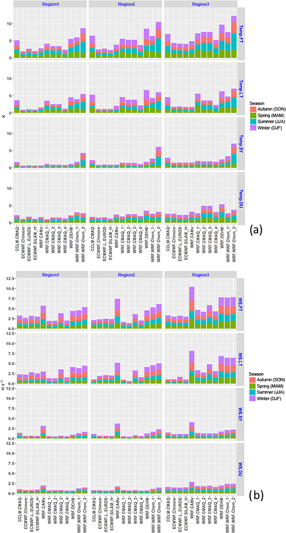
RMSE for (a) temperature and (b) WS in Europe.

The bias for temperature is predominantly negative (model underestimation) for all EU models and subregions, except for WRF-CMAQ4 in EU3, where the model overestimates the measured temperature in summer and winter. According to Katragkou et al. (2015), cold bias during the summer by WRF is typically related to the CAM radiation scheme, and in general the land surface model is pivotal in determining the sign and amount of bias (Mooney et al., 2013). In particular, the combination of NOAH surface scheme and CAM radiation model seems more prone to cold bias.

For NA (Fig. 3a) the temperature RMSE of the WRF-DEHM and CCLM-CMAQ models (peaking in winter and autumn) is ~ 1–1.5 K larger than the WRF-CMAQ model. The error of the SY component is ~ 0.5 K, while that of the DU component is significantly higher (between 0.5 and 2K). The WRF-CMAQ model has a small bias (LT error small) so that the overall error is dominated by the error in the DU component. The bias is negative for the WRF-DEHM model in all subregions and has the same sign for CCLM-CMAQ and WRF-CMAQ, i.e., negative in spring and positive in the other seasons (although for NA2 and NA3 WRF-CMAQ reports a slightly negative bias in winter also, Table S2).

Figure 3.

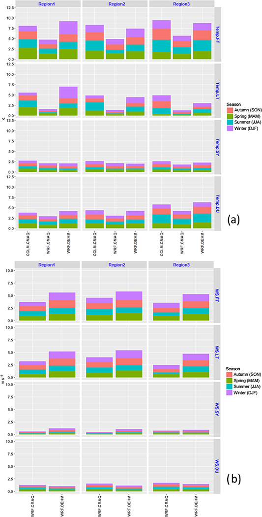
RMSE for (a) temperature and (b) WS in North America.

The RMSE of the surface WS for EU shows large model-to-model variability, more markedly for the LT and SY components (all subregions, Fig. 2b), whereas the error of the DU component is more evenly distributed across models (and significantly higher in EU3, where low wind speed conditions are predominant). Although the meteorological fields are assimilated within the models (either from NCEP or from ECMWF, see Table 2), there are profound differences in the way these fields are ingested and interpolated to the model grid, as well as differences in the parameterization of the boundary and surface layer, which impact the modeled wind speed and temperature. For example, the two instances of WRF-Chem applied the assimilation of the meteorological fields (wind speed, temperature, and relative humidity) of global meteorological fields only above the PBL, whereas other models (e.g., WRF-CAMx) assimilated the global data also within the PBL. For the models directly driven by the global fields, (e.g., SILAM, CHIMERE) the seasonal error for WS (~ 0.5–1 m s⁻¹) and temperature (0.4–1.2 K; Fig. 2a, b) can be considered as the uppermost limit the accuracy of the models can achieve. Thus, the assimilation and interpolation method errors (which are specific to the configuration of the meteorological model) can add more than 1.5 K and 2 m s⁻¹ to the total error.

The full WS time series of the WRF-DEHM, WRF-Chem1 and WRF-Chem2 models report the largest error (in excess of 1.5 m s⁻¹), and the WRF-CAMx model even reports up to 2.4 m s⁻¹ in winter (all subregions, Fig. 2b). On average, the remaining models have an error of 0.5–0.7 ms⁻¹. Most of the error is apportioned to the LT component, with the SY and DU below 0.3 ms⁻¹ (except for WRF-CAMx and the other models mentioned above).

The WS bias is positive for all models (model over prediction), for all seasons and subregions (only exception is the CCLM-CMAQ model, biased low during spring and summer in EU3 and WRF-CMAQ2 during the summer in EU1). The correlation coefficient is above 0.9 for the majority of models and components (except for the models affected by large errors such as the WRF-CAMx model). In general, r is slightly lower in EU3 and is at the maximum for the SY component (Table S3).

For NA (Fig. 3b), the WRF-DEHM model reports an error of ~ 1–1.2ms⁻¹ during all seasons and in all subregions, while the error of the WRF-CMAQ model ranges between 0.45 and 0.75 m s⁻¹ for all seasons and subregions. The error of the SY and DU components is small (below 0.3 ms⁻¹ for each season) for both models. Both models are biased high (all instances) and the correlation coefficient is on the order of ~ 0.9 or above (Table S3).

3.1.2. Vertical profiles of wind speed and temperature

Vertical profiles of mean bias for temperature and WS are reported in Figs. 4 to 7. The modeled profiles were evaluated using ozonesonde measurements. The frequency and local time of the launches are summarized in Table 4. The launches in EU predominately occurred during daylight hours, whereas for NA measurements are also available for nighttime and late afternoon. The sign and magnitude of the bias are informative about error in the PBL processes, which will help discussion on the error of the modeled pollutants (Sect. 3.3).

Figure 4.

Mean bias (model-observations) for the vertical profiles of wind speed measured by ozonesondes launched from the European locations indicated in the inset map of each panel. The number of hourly profiles available for each site is reported in parentheses at the top of each panel.

Figure 7.

Mean bias (model-observations) for the vertical profiles of temperature measured by ozonesondes launched from the North American locations indicated in the inset map of each panel. The number of hourly profiles available for each site is reported in parentheses at the top of each panel.

Table 4.

Summary of ozonesonde data for ozone.

EU
Station	O3 records	Period	Local time
316	52	Year (4–5 launches per month)	11:00–12:00
308	52	Year (4–5 launches per month)	10:00–11:00
318	37	Year (3–4 launches per month, mostly winter and autumn)	11:00–12:00
242	46	January-April (10–12 launches per month)	11:00–12:00
156	144	Year (12 launches per month)	10:00–12:00
099	66	Year (5–6 launches per month)	Mostly early mornings 4:00–6:00
053	149	Year (11–13 launches per month)	11:00–12:00
043	51	Year (4–5 launches per month)	11:00–12:00
NA
021	44	Year (3–4 launches per month)	11:00–12:00
107	54	Year (4–5 launches per month)	16:00–20:00
338	50	Year (2–4 per month; 17 in July; none in September)	14–15 July-17–18 August other months
456	57	2–5 per month; 25 in July	17:00–18:00
457	75	Year (2–5 per month; 18–20 in May-June)	23:00–00:00
458	71	Year (3–8 per month; 20 in July)	23:00–00:00

The bias for temperature in EU ranges between −3K (CCLM-CMAQ at station 308, Fig. 5) and +2K (WRF-CMAQ4 at station 308 and SILAM at station 156) at the surface. In most cases the temperature bias profiles fluctuate around zero (station 053, located between EU1 and EU2; station 043; station 242 in EU2; and partially station 316 in EU2), whereas for some stations the bias keeps the same sign throughout the troposphere, negative for station 156 (launches at 10:00–12:00 LT) and positive for station 099 (early morning launches). The difference in altitudes (491 the former and 1000 m a.s.l. the latter) and the complex terrain of the alpine region might also be responsible for the large model differences at these two (relatively close) stations.

Figure 5.

Mean bias (model-observations) for the vertical profiles of temperature measured by ozonesondes launched from the European locations indicated in the inset map of each panel. The number of hourly profiles available for each site is reported in parentheses at the top of each panel.

Vertical profiles of temperature in NA (Fig. 6) show strong surface bias (negative) at station 021 and 457 (both close to the western border of the domain) for both models. At station 021 (data collected under daylight conditions) the bias becomes positive and small in magnitude above the PBL, whereas at station 457 (data collected under nighttime conditions) the bias keeps the same sign throughout the troposphere. At the other stations, the bias within the PBL is overall small and either positive (107, 456) or slightly negative (stations 458, 338).

Figure 6.

Mean bias (model-observations) for the vertical profiles of wind speed measured by ozonesondes launched from the North American locations indicated in the inset map of each panel. The number of hourly profiles available for each site is reported in parentheses at the top of each panel.

Bias profiles for WS at eight ozonesonde stations in EU (Fig. 4) show a tendency of overestimation in the PBL and of underestimation above ~ 1000 m, although there are some exceptions for different models and/or launching stations. The WRF-Chem1 has the largest positive bias at all sites, with the bias staying positive well above the PBL at all stations in contrast with all other models (WRF-Chem1 model adopted the nudging of meteorological fields only above the PBL and only during the first 12 h of meteorological spin- up, while for the other WRF instances the nudging is active during the entire run). WS overestimation by WRF-Chem is a known concern (e.g., Tuccella et al., 2012; Jimenez and Dudhia, 2012; Mass and Ovens, 2011) and it is likely to have a major impact on the dispersion of pollutants. Similar to EU, the WS bias profiles in NA are biased high near the surface (except for the station 338 and partially station 021, Fig. 6). Above the PBL the tendency is to underestimate the WS (up to ~ 1.5 ms⁻¹), although less dramatically than in EU. Because both NA models are driven by WRF for meteorology, the WS profiles are alike and the magnitude of bias is very similar.

3.2. Wind direction

The spatial and temporal distributions of WD are reported in Fig. 8. The boxes summarize the temporal and spatial variability of the WD values at the receptors of each subregion (no averages were applied). For EU1 (Fig. 8a), the median of all models but WRF-CAMx is within ±5° of the observation, similar to EU2. The modeled 22th and 75th percentiles are also in line with the observations in these two subregions (the CCLM model predicts slightly larger variability).

Figure 8.

Spatial and temporal variability of the wind direction for (a) EU and (b) NA for the full year 2010. The boxes extend between the 25th and 75th percentiles of the total distribution. The whiskers extend from the minimum to the maximum values.

The EU3 subregion is topographically more complex, and the analysis is based on four stations with only 55 % data validity over the entire period. Southern winds are predominant (based on the observation), while the models show large variability and even several instances of WRF (but not all) and ECMWF data tend to underpredict the median value. The only two models that overpredict the median observed value are WRF-CMAx and WRF-CMAQ1; both also apply grid nudging within the PBL along with WRF-CAMQ4, which shows a slight underestimation however.

Results for NA in Fig. 8b show that the modeled WD follows the same distribution as the observed WD, with some excess (or deficiency) of variability by CCLM in NA1 (also the median value is also slightly underestimated) and in NA3. In NA2, all models tend to underestimate the observed median value (CCLM by ~ 20°), indicating a modeled abundance of southerly rotated winds. The WRF-CAMx model for NA, although not reported, uses the same meteorology as WRF-CMAQ and therefore the same WD distribution.

It is difficult to state which error component is more impacted by WD error. The wrong directionality of polluted air masses likely affects the mean value (bias) as well the shape (variance) of the signal since it alters the source-receptor relationship (Vautard et al., 2012; Gilliam et al., 2015). WD error effects on the associativity structure of the modeled-observed time series is less clear however.

3.3. Chemical species: mean square error and error apportionment

3.3.1. CO

CO is a moderately long-lived primary pollutant principally produced by incomplete combustion of fossil fuels, wildfires and, on the global scale, by the oxidation of methane. CO also acts as precursor to ozone. Results of the AQMEII3 models for CO are reported in Figs. 9 and 10 and in Table S5.

Figure 9.

RMSE (ppb) for CO by spectral component and season (panel a for Europe and b for North America). FT is the full (unfiltered) time series, LT, SY, and DU are the long term, synoptic, and diurnal components, respectively.

Figure 10.

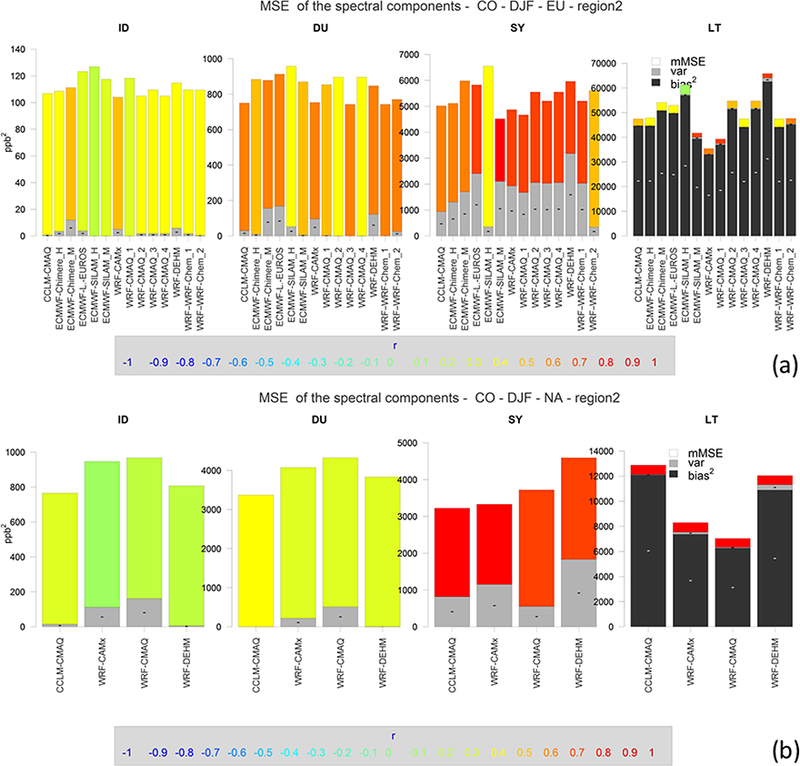
MSE (ppb²) breakdown into bias squared, variance, and mMSE for the spectral components of the spatial average time series of CO during the months of December, January, and February (DJF) based on Eq. (6). The bias is entirely accounted for by the LT component. The signs within the bias and variance portion of the bars indicate model overestimation (+) or underestimation (—) of the bias and variance. The color of the mMSE share of the error is coded based on the values of r, the correlation coefficient, according to the color scale at the bottom of each plot. Top panel is EU; lower panel is NA. Similar plots for the other two subregions are reported in the Supplement.

In general, there are profound differences between the CO statistics for EU and NA, with the latter showing a more marked temporal and spatial dependency as well as model-to-model variability (the yearly mean observed values of CO in EU and NA are of 336 and of 248 ppb, respectively). The EU error (Fig. 9a) is, generally, uniform across models and subregions; it is approximately 3 times higher in winter than in summer. The magnitude of the SY and DU errors is comparable (~ 15–25 ppb on average in EU1 and EU2, sensibly higher in EU3). For NA (Fig. 9b) the DU and SY errors are also similar, but they vary by model, subregion, and season.

The homogeneity of error in EU suggests that it originates from a common source. Previous investigations (Innes et al., 2013; Giordano et al., 2015) indicate that the boundary conditions have a limited contribution to the bias of CO within the interior of the domain where the emissions are far more important. In particular, the MACC inventory used by the EU regional models likely underestimates the CO emissions (especially in winter; Giordano et al., 2015). We conclude that the cause of model bias for CO is most probably attributable to the emissions and to a lesser extent the generally overestimated surface wind speed (Sect. 3.1.1). Sensitivity of the model error to emission changes for CO is discussed in the next section.

The correlation coefficient for EU generally peaks in spring (LT component), while it is at a minimum for the LT component in winter and is overall poor for the DU and SY components. In contrast, for NA the minimum correlation coefficient is observed in spring and summer (LT component), with the correlation for the DU component having a mixed behavior depending on the subregion, but it is typically low in summer (Table S5).

The winter LT error for EU is of ~ 140–220 ppb in EU1 and EU2 and up to 600 ppb in EU3, typically higher than in NA (~ 100 ppb, peaking in autumn and mostly due to model underestimation), while the opposite holds for the DU and ID error, which are significantly lower in EU (Fig. 10) than in NA (except for EU3). Since CO is a primary pollutant, its error is affected by the diurnal dynamics of the PBL height, which is most problematic in winter when modeled PBL has the tendency to become too stable too early, anticipating the evening transition (Pleim et al., 2016). In fact, the biases of CO and those of PM10 (another primary pollutant) in winter are highly correlated for almost all models (not shown), indicating a common cause of the error. The overestimation of WS discussed in Sect. 3.1 also contributes to further dilute the concentration of primary species such as CO (for example correlation (bias_CO, bias_WS) = 0.60 for the CMAQ4 model in EU2 during winter).

The error due to variance in EU (underestimated by the models) and mMSE are significant in the DU and SY components in winter (Fig. 10a). In particular, the variance error of winter DU is small compared to the mMSE, which accounts for almost the entire DU error, up to over 30 ppb. For SY, the model SILAM_H shows an mMSE error of over 75 ppb, the variance part being approximately null. On average, the DU and SY errors are approximately similar for all EU models (~ 45 for DU and ~ 65 ppb for SY), indicating some common error leading to poor associativity, which typically corresponds to lagged timing of the observed and modeled signals. An example of this might be the poor representation of the diurnal variation of the emissions (e.g., Makar et al., 2014). A further reason could stem from the lack of temperature-dependent emissions (the current emission inventory processing approach employs constant temporal emission profiles, and therefore cold-warm episodes are not incorporated in the modeled emissions even though these episodes do affect real-world emissions). The lack of temperature-dependant emissions is likely to have a strong effect for CO since about 50 % of CO emissions comes from residential heating (at least in middle and northern European countries). A test of this hypothesis is currently under investigation by running the CCLM-CMAQ model with a set of emissions using temperature data for the temporal disaggregation for residential heating emissions.

While the SY error is comparable for the two continents, the DU and ID errors are remarkably higher in NA (all subregions, also due to an excess of variance) and for several instances they are comparable or even higher than the LT error. With the exception of the WRF-DEHM model (variance error negligible), the DU and ID errors for the NA models are due to both mMSE and variance.

3.3.2. Sensitivity simulations with reduced emissions and boundary conditions

Additional sensitivity runs were carried out by the majority of modeling groups, in which the amount of anthropogenic emissions were reduced by 20 % in both the boundary conditions and the modeling domain. It is instructive to assess the error variation between the sensitivity runs (denoted as “s20 %”) and the base case for primary species such as CO:

$$\%\mathrm{RMSE}=100\times \frac{{\mathrm{RMSE}}_{\mathrm{CO}}^{\mathrm{s}20\%}-{\mathrm{RMSE}}_{CO}^{base}}{{\mathrm{RMSE}}_{\mathrm{CO}}^{\mathrm{base}}}.$$

Figure 11 reports the error variation for central Europe (subregion EU2), where the effect of local CO outweighs the influence of the CO entering from the boundaries (similar plots for the other two EU subregions are reported in the Supplement). A decrease of 20 % CO produces a RMSE variation of ~ 10 % (averaged over models and components). A naïve projection indicates that a reduction of 100 % (thus removing CO from emissions and boundary conditions altogether) would produce a variation of the error of ~ 50 %. The sign of the error variation indicates that there are circumstances where a reduction of the base case emissions is actually beneficial since the error is reduced (even substantially in the instances where the emissions were overestimated in the base case).

Figure 11.

RMSE variation between the s20% scenario (anthropogenic emission and boundary condition reduced by 20%) and the base case for CO in EU2.

The DU component for CO is the most sensitive to emission changes, with an average of ~ 24 % error variation in summer. The SILAM model is the most sensitive to changes in the amount of pollutants entering the domain. Striking error differences with respect to the base case are detected for summer CO (DU error improved by 50 %), possibly pointing to false peaks in the base case that contribute heavily to the RMSE (as suggested by the low correlation coefficient, Table S5). The reduction of the emission by 20 % lowers the peaks and could be the explanation for the improvement observed for the s20 % scenario for SILAM.

3.3.3. NO

NO is emitted by both natural and anthropogenic sources and its chemistry patterns are closely connected to those of NO₂ and ozone. Due to the fast ozone-NO titration reaction, the uncertainty in emissions, transport, and vertical mixing dominates the uncertainty in chemistry. Since no observational data were available for NA, the discussion is limited to EU. The European Environment Agency (EEA) reports an estimated uncertainty for NO_x emission of ~ 20 % (EEA, 2011); Vestreng et al. (2009) found ±8–25 % uncertainties in EU NO_x emissions, in line with other similar bottom-up uncertainty studies (see Pouliot et al., 2015). A further source of uncertainty and model-to-model difference is the vertical emission profiles adopted and how these are interpolated to the vertical grids used by the models. Within the SILAM model, for example, the vehicular traffic emissions are released largely at the bottom of the first layer. This sub-grid information about the vertical location of the plume used in the vertical transport scheme further suppresses the mixing to the upper layers, thus keeping the surface concentrations higher.

The analysis of the RMSE for NO in Fig. 12a shows how the largest modeling error for NO occurs in winter and autumn, similar in magnitude for EU1 and EU2 (~ 7ppb), while it is more than double in EU3 (up to 30 ppb). The DU and SY errors are comparable in magnitude (although the DU error is slightly higher) and are approximately evenly distributed among the models. For NO the error of the SY component is also model-independent, as noted for CO and as will be discussed for ozone and PM₁₀. Because it is mainly composed of mMSE error (Fig. 12b), it can be hypothesized that the unexplained meteorological variance is responsible for the majority of the SY error.

Figure 12.

Top panel is as in Fig. 9 but for NO (EU only). Lower panel is as in Fig. 10 but for NO (EU only).

The winter bias and variance errors are predominantly negative, indicating model underestimation and reduced variability. The opposite holds for the two instances of SILAM, for which the bias and variance are positive (all subregions). This can be associated with the underestimated ozone concentrations in this model. The applied vertical emission profiles mentioned earlier for this model could also have an influence. The correlation coefficient varies greatly by model, by components, and by season, and it typically degrades for the summer seasons (LT component, most models). The SY component also exhibits low values of r, especially in summer for EU1 and autumn (Table S6). The large variability of the correlation coefficient indicates that the models are not able to capture the fluctuations of this important precursor at all scales.

From the error decomposition plots (Fig. 12b) it emerges that

• - the LT components show a mMSE error approximately uniform for all modeling systems (between ~ 3 and 4ppb);

• - in the majority of cases the mMSE error dominates the ID, DU, and SY components; and

• - the SY component has an error comparable to that of DU for the mMSE part, but it is overall higher due to a predominant lack of variance (as high as 50 % of the total SY error for some models).

Due to its fast chemistry and short traveling distance, the error of representativity for NO (mismatch of the area of representativeness between models with grid spacing of ~ 15 up to 50 km and point measurements) is likely more significant than for other pollutants with a longer lifetime. NO is almost a primary pollutant with negligible deposition (Wesely and Hicks, 2000) and small influence of the boundary conditions (Giordano et al., 2015); therefore, observational sites are affected by local-scale effects in the range of a few kilometers, below the grid spacing of the majority of the models. This has the effect of higher observed mean values compared to the models (enhancing the bias error) and stronger variability in the observations than the models (variance error).

The correlation between the bias of NO and the bias of the other species reveals strong links at several temporal scales (less for the DU timescale though) and also in terms of processes, although it varies greatly by model. For instance, corr (bias_NO, bias_O3) is overall strong (and negative) for the majority of the models but for different timescales, i.e., stronger for the SY components for some models (e.g., LOTOS-EUROS), or for LT (SILAM), or for DU (CHIMERE). Additional analyses are envisioned to determine the causes of such behavior.

3.3.4. Sensitivity simulations with reduced emission and boundary conditions

The analysis discussed in Sect. 3.3.2 is repeated here for NO and results are presented in Fig. 13. A decrease by 20 % of the amount of NO in the domain produces a variation of RMSE of ~ 8 % (averaged over models and spectral components). A naive projection indicates that a reduction of 100 % (thus removing the production of NO from emissions and boundary conditions) would produce a variation of the error of ~ 35 %. Such an amount is less than that found for CO (~ 50 %, Sect. 3.3.2), which is consistent with the photochemical processes involving NO but not CO.

Figure 13.

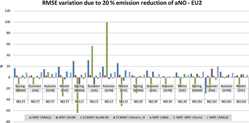
RMSE variation between the s20 % scenario (anthropogenic emission and boundary condition reduced by 20 %) and the base case for anthropogenic NO (aNO) in EU2.

The LT component is the most sensitive to changes for NO, with an average of ~ 17 % error variation (and up to 20 % in autumn, both positive and negative). Again, the SILAM model is the most sensitive to changes in the amount of pollutants entering the domain. Remarkable differences between the s20 % scenario and the base case are detected for summer and autumn (LT error variation of 100 %; Fig. 13). The improvement of the error of SILAM (and of the other models) for the s20 % scenario is due to the overestimation of NO mean concentration in the base case (positive bias, Table S6).

3.3.5. NO₂

Primary NO₂ is emitted by a variety of combustion sources and plays a major role in atmospheric reactions that produce ground-level ozone. NO₂ is also a precursor to nitrates, which contribute to PM formation. As for NO, only a small portion of the total error is expected to stem from the boundary conditions. The AQMEII3 modeling systems attribute a fraction of NO₂ emission ranging between 3 and 10 % of the total NO_x emissions (some models treat the NO₂ emissions from the transport sector differently; see Table 1). The results of the error analysis discussed hereafter do not reveal grouping of model behavior consistent with the choice of the NO₂-to-NO_x emission ratio though, considering the fast chemistry between NO and NO₂.

The RMSE distribution (Fig. 14a, b) shows a marked model-to-model variability in the LT and DU components, while it is more uniform for the SY component, also in the seasonal stratification. Moreover, the error distribution is shown to be weakly dependant on the specific subregion (for both continents, especially for the DU component), suggesting that regional features (e.g., differences in climate between the regions) have little impact on NO₂ performance, which is mostly affected by chemistry and error in the meteorology. Local-scale features (e.g., representation of urban-rural emission differences) may still be important, but they may have similar errors in all regions.

Figure 14.

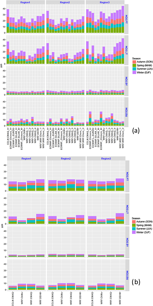
As in Fig. 9 but for NO₂.

The largest error occurs in winter (both continents) and is shared approximately equally between the SY and DU components (for some models the SY and LT errors are comparable due to the small bias).

The bias is the main contributor to the NO₂ error and stems from a model underprediction of the mean observed concentration during the entire year (but, with the exception of the winter season, it is positive for WRF-CMAQ in NA and WRF-CMAQ1 in EU; Table S7). The bias is probably caused by a combination of factors, including emission estimates (e.g., underestimation of residential combustion), PBL height and vertical mixing at night (when wood com bustion emissions tend to be maximum; e.g., Denier van der Gon et al., 2015), and missing processes acting as systematic errors, such as shading effects of forested canopies (e.g., Makar et al., 2016). However, the tendency of NO₂ measurements to be overestimated by the majority of commercially available instruments for detecting NO_x (Steinbacher et al., 2007) needs to be taken into account. The magnitude of the bias is higher in EU (from ~ 1.3 pbb of WRF-CMAQ1 in EU1 to ~ —12.5 ppb of CCLM-CMAQ in EU3) than in NA (the maximum being ~ 5.5 ppb in NA3 by the WRF-DEHM model), with the mean observed values being 11.5 and 10.5 ppb for EU and NA, respectively.

The correlation coefficient is typically higher in spring-autumn and poorer in summer-winter (in summer there are several instances of negative correlation; Table S7). The LT component for EU and the LT and SY components for NA are those with higher correlation coefficients, while SY and DU are the poorest in EU and DU is the poorest in NA (but still higher than ~ 0.4).

The median value of the modeled accumulated deposition per unit area (Fig. S11 in the Supplement) for NO₂ ranges from ~ 0.4 to ~ 1.9 kg km⁻² for EU (nine models) and from ~ 0.3 to 2.3 kg km⁻² for NA (two models). With the exception of the WRF-DEHM model (similar values for EU and NA of 0.3–0.4kgkm^—2), the modeled values for NO₂ deposition are uniform across the EU models, while the deviation between the two NA models for deposition is not negligible, also considering the different native grid sizes of 50 and 12km (WRF-DEHM and WRF-CMAQ, respectively). Therefore, for the majority of the EU models, model-to-model differences in the error are unlikely due to significant difference in the deposition, while differences remain a possibility for NA.

The magnitude of the error for NO₂ resembles that of NO and ozone, although the apportionment reveals significant differences. In fact, while NO includes variance error and a uniform share of mMSE, the LT error of NO₂ for winter is almost completely determined by the bias, for both continents (Figs. 15 and 16). The other NO₂ spectral components (ID, DU, SY) reveal more profound differences with respect to NO, both in terms of bias and of error apportionment. The ID error for NO₂ is even smaller than that of NO (less than 1 ppb) and can be regarded as noise. The DU (~ 1.5 ppb) and SY (~ 1 ppb) errors are also considerably smaller than for NO (both continents), although the DU error presents some excess of variance for WRF-CMAQ3 and the two instances of the CHIMERE model (Fig. 15).

Figure 15.

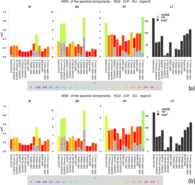
As in Fig. 10 but for NO₂ in EU2. Upper panel is urban sites only (223 stations); lower panel is rural sites only (159 stations).

Figure 16.

As in Fig. 10 but for NO₂ in NA1. Upper panel is urban sites only (39 stations); lower panel is rural sites only (10 stations).

The model-to-model variability of RMSE for the LT component Fig. 15) is very similar to that of NO (Fig. 12), while the DU variability resembles that of ozone (Fig. 18), although for NO₂ the DU error is lower in magnitude and more uniform across seasons.

Figure 18.

As in Fig. 10 but for ozone during the months from May to September.

Moreover, NO_x observations are strongly affected by local emissions and thus the error may stem from the incommensurability of comparing grid-averaged values with point measurements highly affected by local-scale emissions. However, the error apportionment analysis carried out separately for rural and urban background stations (the area type classification is taken for the stations metadata) does not reveal any relevant differences (Fig. 15 for EU2 and Fig. 16 for NA1), if not a slight increase in the variance error over both continents, thus likely excluding chemistry-related model errors.

3.3.6. Ozone

Due to the adverse effects on human health and to the impact on climate, tropospheric ozone is regulated in EU and NA and substantial efforts are made to improve model predictive skill for this pollutant. Tropospheric ozone can be either transported from regions outside the modeled domain, be the result of stratosphere-troposphere exchange, or be produced locally by photochemistry through oxidation of VOCs and CO in the presence of NO_x and sunlight. Due to its photo chemical nature, ozone production is directly influenced by temperature through speeding up the rates of the chemical reactions and increasing the emissions of VOCs (e.g., isoprene) from vegetation (Jacob and Winner, 2009). Along with dry deposition, chemistry can act as a local sink to ozone depending on the photochemical regime.

Results of the AQMEII3 modes for ozone are reported in Figs. 17 and 18 and in Table S4. Overall, the correlation between modeled and observed ozone time series is higher for winter and fall than spring and summer in EU, while the opposite holds true in NA where the maximum correlation is observed in summer (all subregions; Table S4). In EU, the RMSE is generally lower in winter than in the warm seasons (summer and spring; RMSE in summer ranges between 4.3 ppb of WRF-Chem1 in EU1 and 21 ppb of WRF-CAMQ1 in EU3), with the exception of the CCLM-CMAQ model for which the RMSE peaks in autumn (all subregions).

Figure 17.

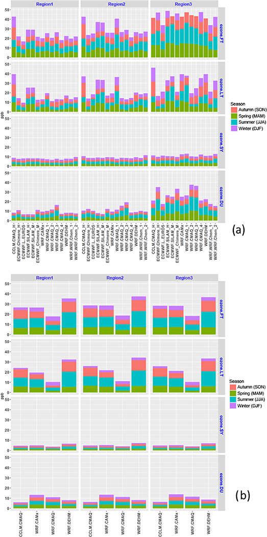
As in Fig. 9 but for ozone.

Due to the strong and well-defined diurnal cycle characterized by ozone formation and loss, the correlation coefficient is generally higher for the DU component, while it tends to be lowest for the SY component (Table S4 and Fig. 18). The SY component often exhibits the lowest correlation among all components, especially in summer (EU) and spring (NA), possibly due to the combined effect of transport of precursors, deposition and chemistry (formation-depletion of ozone from precursor emissions in the regions where the ozone is transported; Bowdalo et al., 2016). However, the SY error is generally small (~ 2–3 ppb, although higher for EU3, where the SY error is double that of the other subregions) and is mostly due to mMSE. It is thus characterized by poor coefficients of determination and underestimated variability (Eq. 6). Therefore, the SY component suffers from low precision (for some models r < 0.3), meaning that the variability of the synoptic mechanisms needs further attention, especially in the meteorological conditions leading to high ozone level episodes and in relation to temperature, cloudiness, and radiation. The WRF-Chem2 model (with the highest error for temperature, Fig. 2b) reports the largest SY error for ozone (especially the variance part). For this model, the correlation between the ozone and the temperature error for the SY component corr (err_O3, err_Temp)_SY is 0.44 for the summer months in EU2 (not shown), which is among the highest; this helps to explain part of the SY error for ozone. Further possible causes could be associated with tropopause folding events, especially downwind of mountain areas (e.g., Bonasoni et al., 2000; Makar et al., 2010), which would also be in line with the larger synoptic error of ozone in EU3 (Fig. S4b), comparable for all models in the range of 3–4 ppb. In order to better characterize the mMSE part of the error for the periodic components, such as DU and SY, analyses of the phase and amplitude are ongoing.

The error of the DU component is largely due to the mMSE term (Fig. 18a), which is comparable for all models in the range of 2–5 ppb, with some significant excess of variance for WRF-CMAQ2 and WRF-CMAQ3 in EU2 (~ 5 ppb). Some possible reasons are the dynamics of the nocturnal PBL and the timing of the ozone cycle, with an either too-fast or too-slow modeled ozone peak (e.g., Pirovano et al., 2012). Limitations of the models to reproduce the amplitude and phase of the daily ozone cycle were already highlighted in the first and second phase of AQMEII, mostly related to the representation of nighttime and stable conditions. Furthermore, the variance error for WRF-CMAQ2 and WRF-CMAQ3 can be induced by the bias of temperature and/or concentration of ozone precursors. For WRF-CMAQ2 (WRF-CMAQ3), corr (err_O3, err_Temp)_DU is 0.88 (0.94) and corr (err_O3, err_NO2)_DU is 0.86 (0.83, summer months, EU2; not shown), which indicates that the errors of the temperature and NO₂ fields are strongly associated with the error of ozone at the DU scale. PBL representation during transitions is a long-standing issue of AQ models.

The error in the LT component is dominated by the bias error (almost completely for NA; Fig. 18), although with significant exceptions in EU (for CCLM-CMAQ the mMSE error of the LT component is larger than the bias portion). The May-September ozone LT bias for EU2 peaks at 12– 13ppb (WRF-CMAQ1), while it is ~ 6ppb in NA3 (but in excess of 20ppb in NA2 by the WRF-DEHM model; the yearly average measured ozone mixing ratio is 26.5 and 29ppb for EU and NA, respectively). The bias of the precursors and of the meteorological fields is typically highly correlated with the bias of ozone. For instance, in EU2 for the WRF-CMAQ1 model, corr (bias_O3, bias_Temp) is 0.65 and corr (biasO₃, biasWS) is 0.81 (summer months). The almost null NO₂ bias for CMAQ1 (among the lowest) combined with the positive bias for NO suggests that chemistry also affects the ozone bias of CMAQ1. Furthermore, the excess of ozone intrusion for the troposphere (discussed next) may also factor in determining the high positive bias at the surface for this model.

According to Bowdalo et al. (2016), the bias of the ozone amplitude cycle linearly evolves with NO_x emissions, suggesting that correction of the error for ozone needs to start from NO_x emissions. Otero et al. (2016) showed that meteorological drivers account for most of the explained variance in ozone, especially over central and northwestern Europe. One of the main drivers of ozone is the daily maximum temperature in relation to the effect of temperature on emissions of VOCs. Therefore, while part of the bias error is possibly due to NO_x emissions, the mMSE and variance error are also likely induced by error in meteorology. Other documented biases are transcontinental transport in winter (Hogrefe et al., 2011) and missing processes during spring and summer, such as the large-scale effect of the absence of forest shading in the models (Makar et al., 2016), a too-rapid production of ozone from available precursors, and an underestimation of ozone deposition (Herwehe et al., 2011). Im et al. (2015b) also indicated a range of factors determining the difference in performance among models, such as the chemical mechanism, biogenic module, and VOC preprocessing, and the difference in microphysics affecting the photolysis, temperature, and radiation that act on the production of ozone.

Although the concentration peaks are associated with the ID and DU components, the contribution to the total error of the ID component is small (<2ppb) due to flattening of the spikes operated by the spatial averaging carried out prior to spectral decomposition. The noise of the ID component is reflected by the correlation coefficient being lower than the correlation of the DU component.

3.3.7. Ozone vertical profiles

Several studies have demonstrated the importance of extending the evaluation of air quality models to the troposphere (e.g., Solazzo et al., 2013; Makar et al., 2010; Herwehe et al., 2011), not only because of the vertical turbulent transport but also for the key role played by coupling of the PBL and the free troposphere in determining the ozone intrusion to the surface. In this section profiles of modeled ozone are compared with ozonesonde measurements.

A summary of the records provided by the ozonesondes for ozone are reported in Table 4. Plots of the simulated and observed ozone levels at fixed heights (through the ENSEMBLE system, models and measurements are paired at the heights of 0, 100, 250, 500, 750, 1000, 2000, 3000, mains through the inflow boundaries. The most significant underestimation (~ 10ppb) is observed at the two stations closer to the western boundary for the EU (stations 318 and 043). The boundary layer deficit of ozone is a long-standing issue, seeing as similar conclusions were derived for the first (Solazzo et al., 2013) and second (Im et al., 2015b; Giordano et al., 2015) phases of AQMEII, as well as for other 4000, 5000, and 6000 m) are reported in Figs. 19 and 20. The ozonesonde data are mainly available during daylight, although two stations with nighttime data are available for NA (Table 4).

Figure 19.

Ozone mixing-ratio profiles measured by ozonesondes launched from the European location indicated in the inset map (lower-right corner) of each panel. The profiles are time averaged over the number of hourly records reported in parentheses at the top of each panel. Legend as in the first panel.

Figure 20.

As in Fig. 19 but for North America.

Overall, the general tendency of the models in both continents is to underestimate the ozone levels above the PBL, suggesting that not enough ozone enters the continental do studies (Katragkou et al., 2015), emphasizing the strong dependence of regional models on the lateral boundary, whose effects propagate far into the interior of the domain.

Towards the interior of the EU domain (stations 134, 157, 242) the profiles are in closer agreement with the observations, with the WRF-CMAQ1 model performing the best throughout the troposphere, possibly due to the overestimation of the entrainment of upper tropospheric ozone, as revealed by the strong gradient of WRF-CMAQ1 at 6000 m (Fig. 19). With respect to the other models (and SILAM in particular), the CMAQ runs show larger ozone availability in the residual layer above the PBL, which acts as a reservoir of ozone that becomes depleted the next day, increasing the concentration at the surface. It is possible that the PBL and vertical mixing within these models is too weak (Appel et al., 2016). Further analyses restricted to specific season and time of the day are required to validate this hypothesis.

For NA (Fig. 20), the general tendency is of slight-to-consistent (stations 71 and 75) overestimation within the PBL, underestimation for the WRF-CMAQ model, over estimation (stations 107, 456, and 458 - afternoon-night launches) at the surface, and mild underestimation above the PBL for the WRF-DEHM model.

3.3.8. Relationship between the bias of ozone, NO_x and Temperature

The relationship between the bias of NO and the bias of ozone is reported in Fig. 21 for the EU2 region (similar plots including the bias of NO₂ for EU and NA are provided in the Supplement). A linear relationship between the biases of the two species is detectable, which is more evident in winter. Large positive ozone bias is driven by underestimation of NO (a primary species), whereas the largest negative ozone bias corresponds to the largest overestimation of NO. The role of the temperature bias is less clear, but the NO₂ and ozone relationship (Fig. S7) suggests that large NO₂ bias is associated with temperature underprediction. The partition of NO_x emission into primary NO and NO₂ seems to suggest that the models adopting a 95 / 5 % ratio suffer lower ozone bias (at least in winter), although in general the clustering of models based on the NO / NO₂ share of total NO_x emission is far from robust. A simple linear regression between NO bias and ozone bias (based on the yearly time series) among the EU models suggests that the NO_x and temperature biases can explain, on average, ~ 35 and ~ 16 % of the variability of the ozone bias, respectively.

Figure 21.

Ozone vs. NO modeled mean bias for the EU2 subregion, color-coded by temperature bias and symbols according to the NO_x emission fraction of NO and NO₂. Each point represents a model. (a) Winter months and (b) summer months.

3.3.9. SO₂

SO₂ is another primary regulated pollutant, which in EU and NA, is mainly emitted from coal power plants and also from the residential heating and waste disposal sector. SO₂ acts as a precursor to sulfates, which are one of the main components of PM in the atmosphere. Any error in SO₂ is likely inherited by these secondary species. The majority of models employed the prescribed vertical distribution by EMEP (_S1_Reference162Vestreng and St0ren, 20_S1_Reference16200), while CMAQ4 in EU and WRF-CMAQ in NA adopted the Briggs plume rise algorithm (Briggs, 1971,1972) accounting for the effects of modeled meteorology. SILAM, CHIMERE, and CCLM-CMAQ adopted the sector-dependent vertical emission profiles as in Bieser et al. (2011b). The EEA reports an estimated uncertainty for SO₂ emission of ~ 10% (EEA, 2011); therefore, SO₂ emissions are expected to be more accurate than NO_x emissions. This is reflected in the low bias in both continents (~ 1–2 ppb in winter, mostly due to model underestimation; Figs. 22 and 23). The averaged observed concentration of SO₂ is 1.92 and 2.7 ppb in EU and NA, respectively.

Figure 22.

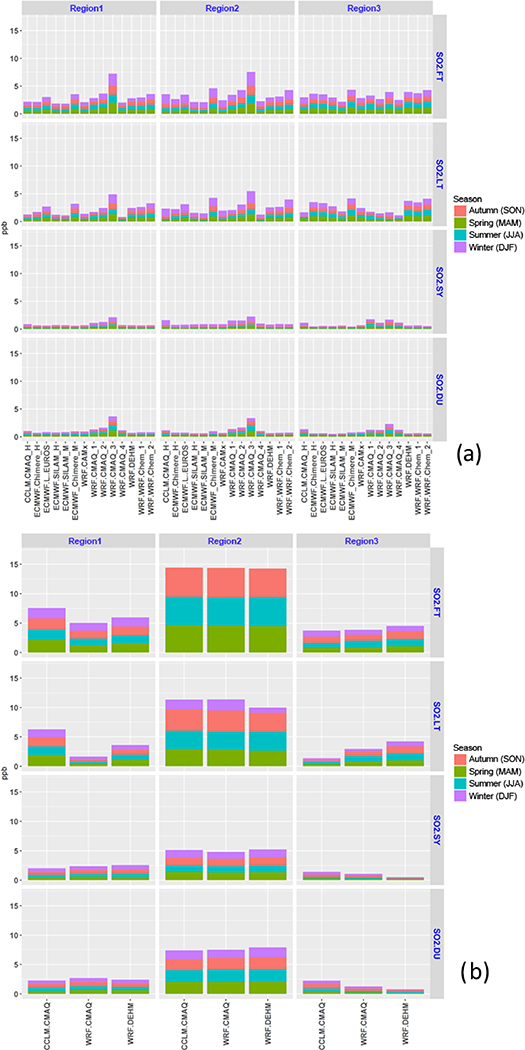
As in Fig. 9 but for SO₂.

Figure 23.

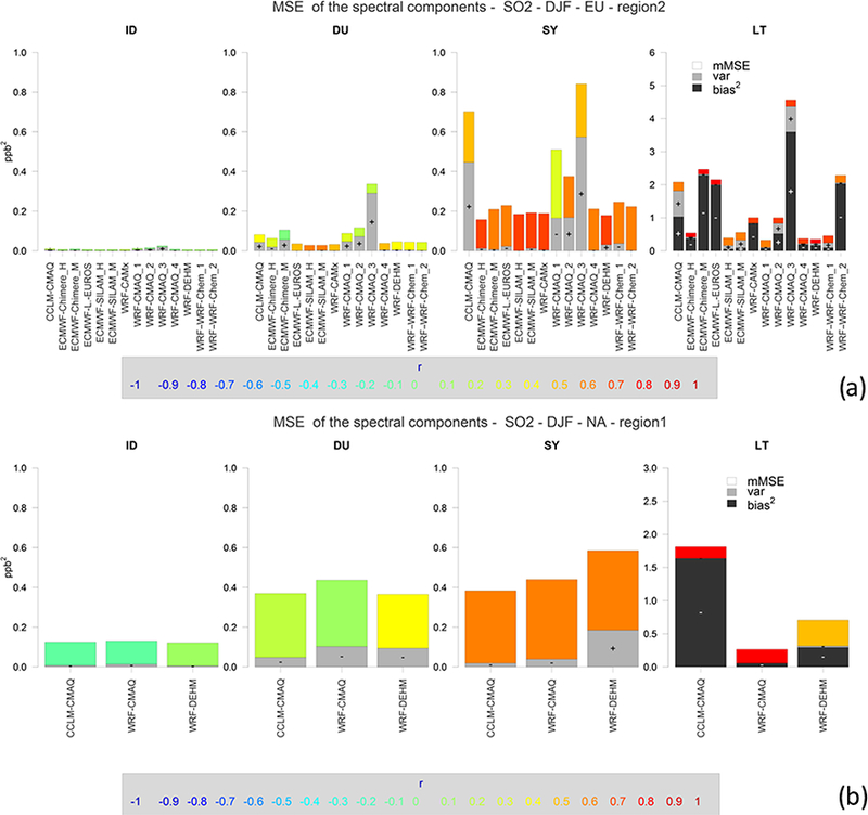
As in Fig. 10 but for SO₂.

The seasonal modeled error for SO₂ ranges, on average, between 0.65 and 1.3 ppb in EU and between in excess of ~ 1 and 5 ppb in NA (the maximum error in NA2), peaking in autumn.

In EU and NA1, the error of the ID, DU, and SY components is comparable for all seasons and is, on average, below 0.6 ppb. There are some exceptions, most notably the WRF-CMAQ3 model, which is the only one biased significantly high (Fig. 23a) and it shows an excess of variance significantly larger than the other models. By contrast, WRF-Chem2, CHIMERE, and LOTOS-EUROS shows significant low bias (the latter two models have the smallest number of vertical layers). Overall, though, the bias error does not group consistently by PBL scheme and/or vertical resolution. For example, CMAQ2, CMAQ3, and CMAQ4 employ the same PBL scheme based on ACM2 and have a comparable number of vertical levels (CMAQ3 has even more), but the bias of CMAQ3 is much larger than that of CMAQ4 and CMAQ2, which in turn have comparable bias but opposite in sign. The two instances of WRF-Chem show significantly different bias, which might be due to the different PBL and cloud schemes, influencing the SO₂ oxidation (Table 2).

The large variability of the model-to-model error (especially in EU) and correlation coefficient for both continents is an indication that the mechanisms governing the initial mixing and subsequent transport and chemical transformation suffer from different sources of error at all scales. In no instance is the correlation coefficient consistently above 0.5 for all seasons and spectral components, while there are several instances of negative correlation between the spectral components of observed and modeled SO₂ (e.g., CCLM-CMAQ model in EU and several others). The poor correlation coefficient of especially the ID and DU components for both continents indicates that the peaks of the SO₂ concentration are not caught by the models, leading to low precision. Although the mean fluctuations are generally well reproduced (low variance error for both continents), there remains a significant portion of unexplained variance (mMSE) error, which can derive from meteorology and chemistry. Bieser et al. (2011b) showed that the height of the release and vertical distribution of the SO₂ emissions influence the SO₂ / SO₄ ratio since the oxidation (aging) of SO₂ is more effective if the emissions are higher up. Since power plants are the major source of SO₂, further analysis should investigate the impact of differences in the vertical emission distribution between models.

3.3.10. Particulate matter

PM, in both the fine and coarse fraction, is directly emitted by biomass and fossil fuel combustion in domestic and industrial activities, and it is also formed from precursors in the atmosphere.

From the AQMEII3 suite of model runs, the error for PM is evaluated for PM₁₀ in EU and PM_2.5 in NA. The choice is dictated by the availability of hourly measurements in the two continents. The RMSE distribution is reported in Fig. 24 (PM₁₀ for EU) and Fig. 25 (PM_2.5 for NA). The error distribution for EU reveals that despite the large number of modeling options and parameters characterizing the chemistry and physics of particles, the error distribution for DU and SY is homogeneous among the EU models. For these components the error is approximately uniform over seasons, although with some exceptions (it is significantly higher in EU3, although this is based on two receptors only). EU3 is a small area compared to EU1 and EU2, but it is densely populated, intensively farmed, and has a large amount of wood burning in winter and agricultural area in summer. It is surrounded by mountains and stagnant flow conditions are predominant. Thus, it is a challenging area for current modeling systems, especially for primary species such as PM.

Figure 24.

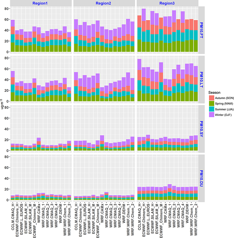
As in Fig. 9 but for PM10 in Europe (error units in μg m⁻³).

Figure 25.

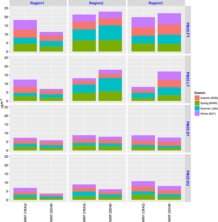
As in Fig. 9 but for PM2.5 in North America (error units in μg m⁻³).

The LT component shows some significant model-to-model variations due to the WRF-CAMx and WRF-CMAQ1 models, which have a lower error in spring and summer compared to the other models, while the CCLM-CMAQ model has a higher LT error in EU1.

The magnitude of the SY error in EU is on average ~ 6μgm⁻³ during winter, with a peak of 10.5μm⁻³ in EU2 (WRF-CAMx model). The magnitude of the DU error is lower (~ 2–2.5 μg m⁻³ in EU1 and EU2, and ~ 5–6 μg m⁻³ in EU3), with the largest share in autumn, spring, and winter and slightly lower in summer. The error of the LT component ranges between ~ 11 and 15 μg m⁻³ in EU1 and EU2 and up to 25 μg m⁻³ during winter in EU3.

The analysis of the correlation coefficient reveals that the model-to-model differences in the correlation coefficient with the observed component time series tend to be most pronounced for the DU and ID components, indicating that these two components are pivotal in determining the overall model skill in terms of capturing observed fluctuations in PM₁₀ concentration. In more detail, the correlation is poor for the DU component (especially in EU2 and EU3, Table S9), possibly due to PBL dynamics and emission profiles (as discussed above for the RMSE at the DU scale). The LT component has correlation values varying highly among models and among seasons for the same model (e.g., the LT correlation of the WRF-CMAQ4 model in EU3 is ~ 0.9 during spring but only 0.35 in summer).

In winter the LT and SY error is more severe, likely due to the larger uncertainties in PM₁₀ emissions of combustion processes (wood burning, residential heating), as well as due to the current limitations in modeling the vertical mixing during stable conditions, as mentioned for the gaseous species (especially CO, being another primary species). The majority of the EU models show an LT error in winter between 12 and 16μgm⁻³, eight models above 16μgm⁻³, and only one (WRF-CAMx) below 10 μg m⁻³. The absence of background sea salt for all EU models (see end of Sect. 2.3) can also be responsible for low bias of the LT component for PM₁₀, especially in the vicinity of the coastline.

The SY winter error exceeds 5μm⁻³ for all models (all subregions) and three instances (WRF-CAMx, WRF-Cheml, and WRF-Chem2, the latter showing the highest accumulated deposition for PM₂.5; Fig. S11) report an error above 7.5 pg m⁻³, possibly due to the low nitrate concentration and high sulfate concentration during winter months, resulting from the GOCART parameterization of the aqueous cloud chemistry. All the remaining models have comparable mMSE and variance errors (Fig. 26) and are biased low (model underprediction), possibly due to missing PM source and overestimated surface wind speed. As for the WRF-CAMx model, the low bias on the LT component and the relatively high mMSE error in the SY fraction suggest that the model was able to capture the mean magnitude of PM concentration over the entire year, but it failed in reconstructing the correct variability of the different episodes, whose timing is generally driven by the synoptic timescale.

Figure 26.

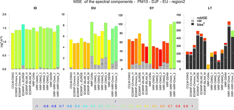
As in Fig. 10 but for PM₁₀ in Europe (error units in μg m⁻³).

The analysis of corr (bias_Temp, bias_PMl0)lt shows that the error of these two variables is related, especially during the spring months and more consistently in EU3 (up to 0.74 for the WRF-Cheml model) and during autumn in EU1 (the bias of temperature and the bias of PM10 are anticorrelated up to −0.67 for CMAQ1). Conversely, other models (e.g., the CAMx model) do not show any significant correlation.

The PM_2.5 evaluation for NA is restricted to two models, WRF-DEHM and WRF-CMAQ, which show comparable error (Fig. 25). The WRF-CMAQ (WRF-DEHM) model has an error ranging between ~ 3.5 (~ 2) and ~ 6 (~ 8.5) μm⁻³. The main contribution to the total error stems from the LT component (predominantly negative bias) and from the SY component (2–3 μm⁻³). The DU component contributes to about 1.5 μm⁻³ (comparable mMSE and variance error).

Both NA models are biased low in summer (all subregions), which can be attributed to limitations in the SOA mechanism (Zare et al., 2014). Because of the higher contribution of primary PM₂.5 to total PM₂.5 during winter, differences in horizontal and vertical resolution (Table 1) likely contribute to the difference in winter LT bias. The correlation coefficient for the two models is generally higher in winter (full time series) and deteriorated for the DU component (all seasons and subregions).

As inferred for the species discussed above, the uniformity of model behavior is indicative of errors stemming from external fields, likely emissions, where missing sources of PM can affect the error within certain timescales for all models. Further common causes of error are intrinsic to the model-observation comparison because modeled PMs are commonly dry, while this is not always the condition for the measurements. For instance, the filter-based gravimetric measurements as recommended by the European Committee for Standardization (CEN) are likely to retain part of the particle-bound water after filter conditioning at a constant temperature of 20 ⁰C and relative humidity of 50 %. Recent findings by Prank et al. (2016) report the aerosol water content from the gravimetric measurements to range between 5 and 20 % for PM2.5 and between 10 and 25 % for PM₁₀. The particle-bound water was found to be associated with hygroscopic particles such as sulfate, nitrate, and organic compounds. This remaining water content can be up to approximately 10–35 % depending on the chemical composition of aerosols being measured (Tsyro, 2005; Kajino et al., 2006; Jones and Harrison, 2006). The water aerosols should therefore be accounted for when compared with these measurements. Part of the problem lies in secondary organic aerosol. In winter, in particular for the wood burning part of the emissions, there are condensable gases that rapidly change to the aerosol phase but are missed since they are not part of the presently used PM emission inventory. In summer, biogenic emissions that contribute to SOA formation and their yields are quite uncertain. A good representation of SOA is still a problem for all models. In spring, the application of manure and fertilizer leads to peaks of NH₃ emissions and subsequent NH4 aerosol formation, contributing to PM₁₀ and PM_2.5. The timing of these emissions is parameterized based on long-time averages, whereas in practice they are strongly related to meteorology. This can explain part of the discrepancy between the diurnal and synoptic timescales (Hendriks et al., 2016).

4. Memory of the signal and removal processes: the case of ozone

The evaluation of the removal processes (chemical transformation, transport, and deposition) is difficult to assess in isolation with respect to other sources of error because of the bias of the signal. In this section we propose a bias-independent spatial analysis aimed at the quantification of the memory of the signal. The analysis seeks the time interval (or memory) after which the signal loses any memory of its past. The memory of the modeled and observed signals is then compared. The methodology consists of

1. calculating the autocorrelation function (acf) of the modeled and observed LT components;

2. calculating the quantity acf_mod=o and acf_ob_s=o, i.e., the lag (time interval) where the acf of the modeled and observed LT components falls to zero; and finally

3. determining the difference between the two, which yields the difference between the modeled and observed memory of the signal:

   $${\Delta }_{\mathrm{memory}}={\mathrm{acf}}_{\mathrm{mod}}{}_{=0}-{\mathrm{acf}}_{\mathrm{obs}}{}_{=0}.$$ (9)

The acf is simply a measure of the degree of associativity of a time series with its lagged version. The associativity is typically measured through the correlation coefficient, and the lag extends from one time step (1 h in the case of hourly time series) to one-third of the length of the time series. Because the correlation is bias-independent, we conclude that the acf is also bias-independent; therefore, information from A_memory is useful for the interpretation of the variance and covariance errors discussed in Sect. 3.1. The memory of the signal is different from the persistence indicator (previous day concentration) as used by Otero et al. (2016), for example, for accounting for pollutant episodes. As we deal with the LT component of the signal, short-term and synoptic episodes are in fact filtered out in this analysis.

In Figs. S9 and S10, the acf for the network-wide spatial average and for the full year are reported. The acf is calculated for the LT component of the observed (first panel) and modeled ozone time series. The zero of the acf and the slope of the decay of acf of the observations (approximately a straight line from 1 to 0 in 2000 h) are replicated by the models with various degree of success (Fig. S10). Our intent is to apply this analysis to the seasonal ozone time series at each receptor and derive useful information about the modeled removal-production processes. The spatial analysis is proposed for ozone for the months of May to September (Figs. 28 and 29) and for the full year (Figs. S9 and S10).

Figure 28.

Spatial map of the ozone monitoring stations colored based on the “delta hour” values, i.e., the difference in hours between the zero of the autocorrelation function (acf) for the modeled ozone minus the zero of the acf of the observed one. The acf is calculated on the long-term component for the months of May to September. Negative values indicate too-short memory and excess of removal (vice versa for positive values). The box on the right summarizes the delta hour percentile distribution.

Figure 29.

As in Fig. 28 but for North America.

The average lifetime of ozone in the troposphere is of approximately 20–30 days (Solomon et al., 2007). By analyzing the LT component (processes > ~ 21 days), we therefore screen out the daily removal-transformation due to chemistry and can focus on seasonal transport, deposition of the free tropospheric ozone, long-term chemistry (seasonal changes in vegetation that affect biogenic VOC emissions and ozone deposition, and also the monthly variations applied to the anthropogenic emission), and influence of boundary conditions. The structure of the acf also benefits from the removal of short timescale processes because it is less affected by noise and the results are easier to interpret.

The spatially distributed Δ_memory shows some clear regional effects for the majority of the models. The Δ_memory > 0 along the Mediterranean coast of Spain and France, with some severe excess of ozone production (or underestimation of sinks) in southern-central France for some models (SILAM, WRF-CAMx, WRF-CMAQ1, WRF-CMAQ2, and especially the LOTOS-EUROS model, for which the acf at the French receptors did not reach zero).

The region covering the Po Valley, Italy, and extending into continental eastern EU is affected by negative Δ_memory (sometimes a deficit of 1 month for some models). The negative memory indicates that the observed signal is more persistent than the modeled one and that long-term weather transitions are smoother in gradient and longer in duration. Thus, the seasonal modulation of the signal is overestimated by the models, which produces variance error. Coupling the two behaviors (excess of ozone in southern France and southern Spain with the short memory from the interior of eastern EU extending to the Po Valley) might indicate an easterly synoptic transport of ozone (or of LT ozone precursor, such as the impact of CH₄ and CO on OH and photochemistry) masses whose duration is underestimated by the models. The relationship between the sign of A_memory and the land use type (vegetation vs. urban) is the subject of ongoing investigations in the attempt to determine the role of VOC emissions and deposition over different land types.

The central part of Germany is affected by positive (on average in the range of 7 to 10 days) Δ_memory, mostly visible for the HTAP-emission-based SILAM and CHIMERE results, in contrast with the MACC-emission-based results of the same models. When the HTAP inventory is used, the largest differences are observed in central EU regions, indicating that the LT chemistry also plays a role.

The deposition aspect of removal can be as equally important as transport and chemistry. The memory of the signal directly depends on the amount of ozone available and a large negative Δ_memory might indicate that the deposition is too high.

For NA (Fig. 29), the feature common to all models is the excess of removal on the southern Atlantic coast and across the eastern Canadian border. In contrast, the central-eastern part of the US shows large positive Δ_memory values (up to ~ 1.3 month for the WRF-DEHM model), with the exception of the WRF-CMAQ model, which is overall in line with the observed memory of the signal in this part of the domain. This result agrees with the seasonal phase analysis for ozone in global models by Bowdalo et al. (2016), where a delay of up to 4 months was detected for the eastern US.

The west coast has a mixed behavior, but Δ_memory is prevalently negative. The hypothesis that too little ozone enters the domain through the boundary conditions is contradicted by the Δ_memory ~ 0 for a full year on the west coast (seeFig. S10). A potential excess of transport in this region also seems to be contradicted by the large number of stations for which Δ_memory is positive. A possible conclusion is that localized biogenic emission sources, radiation budget, and deposition are the main factors responsible for the negative sign of Δ_memory in this region.

5. Conclusions

The work presented in this paper summarizes the results of the third phase of the AQMEII activity focusing on AQ model evaluation, applied to the continental-scale domains of Europe and North America. The evaluation of the AQMEII3 suite of model runs is carried out for surface temperature, wind speed, and direction and for the species CO, NO, NO₂, ozone, SO₂, PM₁₀ (EU), and PM₂.5 (NA). Additional analyses making use of emission reduction scenarios (CO and NO) and vertical profiles were also performed.

This work is primarily meant to provide a wide overview of the performance of current regional AQ modeling systems and to set the basis for additional diagnostic analysis that is currently in progress.

The model evaluation is carried out by quantifying the components of the error (bias, variance, mMSE) at four timescales (ID, DU, SY, LT), each describing physical processes in a specific time range. The bias and variance measure the departure from the first and second moment of the observed distribution (mean and standard deviation), while the mMSE accounts for the unexplained observed variability. The apportionment of the error to the relevant timescales and the analysis of the quality of the error revealed that the LT bias is by far the biggest cause of error, followed by the variance error (fluctuations about the mean value) of the DU component and the unexplained variance of the DU and SY components, depending on the species and season. In more detail:

• - The mean concentration of the primary species (NO, CO, PM₁₀, SO₂) is underestimated by the vast majority of the models on both continents, more markedly during the winter and autumn seasons. The largest share of error for these species is the bias of the LT components, most probably due to error of the fluxes at the boundaries (emission, deposition, and boundary conditions) and to the effects of comparing point measurements to volume-averaged concentrations.

• - The bias is by far the primary source of error and the most important from a model evaluation-development point of view. Because it is essentially a shift of the mean concentration, the causes of it need to be sought in processes and conditions at the boundaries that have a systematic effect of displacing the concentration values while approximately preserving the shape of the distribution. Thus, processes like emission timing, chemistry transformation, autocorrelation structures, stratospheric intrusion, and atmospheric stability are not likely responsible for systematic bias-type error (though they can be a source of casual inaccuracy for limited periods). Conversely, deposition fluxes, magnitude of emission, and input from the lateral boundaries are more probable sources of bias error. The effect of meteorology is more complex because errors in synoptic circulation can cause surface wind velocity and direction to be inaccurate, and thus negatively impact the long-term modeled concentrations, causing bias error.

• - The meteorological fields of temperature and wind speed are consistently biased low and high, respectively. Based on the results of the European models directly driven by the global fields for meteorology (e.g., SILAM, CHIMERE), the error for wind speed is of ~0.5–1 ms⁻¹ and of ~0.4–1.2K for temperature. These errors can be considered as the uppermost limit the accuracy of the models can currently achieve. The use of nudging and interpolation methods (specific to the configuration of the meteorological model) can add more than 1.5 K and 2 m s⁻¹ to the total error. The analysis of the available vertical profiles suggests that the models overestimate the wind speed within the PBL and vice versa above the PBL, possibly inducing a net outward flux of pollutants at the PBL interface.

• - Modeled CO is affected by high errors, uniformly across models and components and more pronounced in winter. It is also predominantly driven by the negative bias of the LT component, followed by variance error of the SY component. Modeled NO and NO₂ also report negative bias but in contrast to CO, there is significant model-to-model difference in error variability, possibly due to the chemistry of NO_x. The SY and DU errors of NO are comparable in magnitude (3–5 ppb) and mostly due to mMSE error. Preliminary sensitivity investigations for CO and NO seem to suggest that at most ~ 50 and ~ 35 % of the total error, respectively, could be due to emissions.

• - The error analysis for ozone shows large model-to-model variability for all errors and spectral components, with the exception of the SY component for which the error is similar among models and possibly driven by the error in temperature and in the boundary conditions. This is because modeled vertical ozone profiles near the domain’s boundaries are typically underestimated in both continents by all models. The bias is prevalently positive, while the variance error is generally small. While the bias error for ozone is likely driven by error in NO_x emissions, the error in meteorology may factor in determining the mMSE and variance error. In fact, there are several models for which the bias of temperature and the bias of NO₂ are strongly associated with the DU error of ozone. A simple linear regression between NO_x bias and ozone bias (based on the yearly time series) among the EU models suggests that the NO_x and temperature biases can explain, on average, ~ 35 and ~ 16 % of the variability of the ozone bias, respectively. Ongoing analyses are focusing on explaining the origin of the mMSE error by investigating the phase shift between the modeled and observed DU and SY components as well as focusing on looking at maximum daily values rather than at the full time series.

• - PM analysis (PM₁₀ for Europe and PM_2.5 for North America) reveals that for Europe the error distribution for DU and SY is homogeneous and season independent among the models, despite the large numbers of modeling options and parameters characterizing the chemistry and physics of particles. A common source of model bias (model underestimation, especially in winter) for PM10 likely lies in the emissions (missing sources) and in the overestimation of surface wind speed, whereas variance error may stem from PBL dynamics under stable conditions and missing processes in the model (SOA formation is a known issue for all models). The analysis of PM_2.5 (based on two models only) shows an excess of variance and low correlation coefficient in the DU component, possibly due to the timing of the PM cycle. Further analyses dealing with the PM components are needed.

• - The analysis of the memory of the ozone signal has revealed a strong model deficit in continental Europe, where the seasonal modulation of ozone is overestimated by the majority of the models. The opposite holds true in the continental US.

Although remarkable progress has been made since the first phase of AQMEII, both in terms of model performance and in terms of developing a more versatile and robust evaluation procedure, results of AQ model evaluation and intercomparison remain generic since they fail to associate errors with processes, or at least to narrow down the list of processes responsible for model error. AQ models are meant to be applicable to a variety of geographic (and topographic) scenarios under almost any type of weather, season, and emission conditions. For such a wide range of conditions the inherent nonlinearity among processes is difficult to disentangle, and specifically designed sensitivity runs seems to be the only viable alternative. A model evaluation strategy relying solely on the comparison of modeled vs. observed time series would never be able to quantify exactly the error induced by biogenic emissions, vertical emission profiles, or their dependence on temperature, deposition, and vertical mixing, for example, and the analyses presented in this work are no exception. In fact, the methodology devised to carry out the evaluation activity in this study has not succeeded in determining the actual causes of model error, although it does provide much clearer indications of the processes responsible for the error with respect to conventional operational model evaluation.

The highly nonlinear nature of current AQ models requires the study of the relationships among error fields, meteorological drivers, and precursors. When the seasonal and spectral structures of these relationships are analyzed together with the error of the input fields (emissions and boundary conditions), then it would be possible to diagnose and accurately explain the processes responsible for the error. Future AQ model evaluation activities should envision sensitivity simulations and process specific analyses. The “theory of evaluation” based on information theory currently being developed by the hydrology modeling community (Nearing et al., 2016, and references therein) is a promising way forward and the AQ community should be prepared for those developments.

Ongoing work (Solazzo et al., 2017) is being devoted to deepening the investigation into causes of model errors by focusing on two models (CMAQ for NA and CHIMERE for EU), for which additional model runs were carried out to frame the effect of fluxes (emissions, boundary conditions, and deposition) on modeled ozone.

Figure 27.

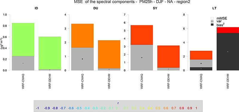
As in Fig. 10 but for PM2.5 in North America (error units in μg m⁻³).

Appendix A

Following Hogrefe et al. (2000) and Galmarini et al. (2013), the time windows (m) and the smoothing parameter (k) were selected as follow:

$$\begin{gathered} \mathrm{ID}(t)=x(t)-{\mathrm{kz}}_{3,3}(x(t)) \\ \mathrm{DU}(t)={\mathrm{kz}}_{3,3}(x(t)-{\mathrm{kz}}_{13,5}(x(t)) \\ \mathrm{SY}(t)={\mathrm{kz}}_{13,5}(x(t))-{\mathrm{kz}}_{103,5}(x(t)) \\ \mathrm{LT}(t)={\mathrm{kz}}_{103,5}(x(t)) \\ \hspace{0.17em}\hspace{0.17em}\hspace{0.17em}x(t)=\mathrm{ID}(t)+\mathrm{DU}(t)+\mathrm{SY}(t)+\mathrm{LT}(t), \end{gathered}$$ (A1)

where x(t) is the time series vector. The additive property of the components whose summation returns the original time series might be questioned. In the original work by Rao et al. (1997) the importance of log-transforming the components to stabilize the variance is highlighted. In the case of log-transformation, the original time series is obtained by the product of exponential functions whose exponents are the spectral components. For the purposes of the error apportionment analysis presented here, the results of using the additive time series component of log-transformation did not produce substantial differences.

A clear-cut separation of the components of Eq. (A1) is not achievable since the separation is a nonlinear function of the parameters m and k (Rao et al., 1997). It follows that the components of Eq. (A1) are not completely orthogonal and that there is some level of overlapping energy (Kang et al., 2013). Galmarini et al. (2013) found that the explained variance by the spectral components accounts for 75 to 80 % of the total variance, the remaining portion coming from the interactions between the components.

Appendix B

Statistical indicators are as follows: root mean square error as

$$\mathrm{RMSE}={\left(\frac{{\displaystyle {\sum }_{i=1}^n{(M_i-O_i)}^2}}{n}\right)}^{0.5},$$

mean bias (MB) as

$$\mathrm{MB}=\frac{1}{n}{\displaystyle {\sum }_{i=1}^n{M}_i-O_i,}$$

and Pearson correlation coefficient (r) as

$$r=\frac{1}{n-1}{\displaystyle {\sum }_{i=1}^n}\left(\frac{M_i-\overline{M}}{{\sigma }_M}\right)\left(\frac{O_i-\overline{O}}{{\sigma }_O}\right),$$

where M and O are the n element-modeled and -observed time series, respectively, O is the standard deviation, and the overbar indicates temporal averaging.

References

- Ackermann IJ, Hass H, Memmsheimer M, Ebel A, Binkowski FS, and Shankar U: Modal aerosol dynamics model for Europe: development and first applications, Atmos. Environ, 32, 2981–2999, doi: 10.1016/S1352-2310(98)00006-5, 1998. [DOI] [Google Scholar]
- Ahmadov R, McKeen SA, Robinson A, Bahreini R, Middlebrook A, de Gouw J, Meagher J, Hsie E, Edgerton E, Shaw S, and Trainer M: A volatility basis set model for summertime secondary organic aerosols over the eastern United States in 2006, J. Geophys. Res, 117, D06301, doi: 10.1029/2011JD016831, 2012. [DOI] [Google Scholar]
- Ahmadov R, McKeen S, Trainer M, Banta R, Brewer A, Brown S, Edwards PM, de Gouw JA, Frost GJ, Gilman J, Helmig D, Johnson B, Karion A, Koss A, Langford A, Lerner B, Olson J, Oltmans S, Peischl J, Pdtron G, Pichugina Y, Roberts JM, Ryerson T, Schnell R, Senff C, Sweeney C, Thompson C, Veres PR, Warneke C, Wild R, Williams EJ, Yuan B, and Zamora R: Understanding high wintertime ozone pollution events in an oil- and natural gas-producing region of the western US, Atmos. Chem. Phys, 15, 411–429, doi: 10.5194/acp-15-411-2015, 2015. [DOI] [Google Scholar]
- Appel KW, Pouliot GA, Simon H, Sarwar G, Pye HOT, Napelenok SL, Akhtar F, and Roselle SJ: Evaluation of dust and trace metal estimates from the Community Multiscale Air Quality (CMAQ) model version 5.0, Geosci. Model Dev, 6, 883–899, doi: 10.5194/gmd-6-883-2013, 2013. [DOI] [Google Scholar]
- Appel KW, Napelenok SL, Foley KM, Pye HOT, Hogrefe C, Luecken DJ, Bash JO, Roselle SJ, Pleim JE, Foroutan H, Hutzell WT, Pouliot GA, Sarwar G, Fahey KM, Gantt B, Gilliam RC, Kang D, Mathur R, Schwede DB, Spero TL, Wong DC, and Young JO: Overview and evaluation of the Community Multiscale Air Quality (CMAQ) model version 5.1, Geosci. Model Dev. Discuss, doi: 10.5194/gmd-2016-226, in review, 2016. [DOI] [PMC free article] [PubMed] [Google Scholar]
- Banzhaf S, Schaap M, Kerschbaumer A, Reimer E, Stern R, van der Swaluw E, and Builtjes P: Implementation and evaluation of pH-dependent cloud chemistry and wet deposition in the chemical transport model REM-Calgrid, Atmos. Environ, 49, 378–390, doi: 10.1016/j.atmosenv.2011.10.069, 2012. [DOI] [Google Scholar]
- Beltman JB, Hendriks C, Tum M, and Schaap M: The impact of large scale biomass production on ozone air pollution in Europe, Atmos. Environ, 71, 352–363, doi: 10.1016/j.atmosenv.2013.02.019, 2013. [DOI] [Google Scholar]
- Bergstrom R, Denier van der Gon HAC, Prdvot ASH, Yttri KE, and Simpson D: Modelling of organic aerosols over Europe (2002–2007) using a volatility basis set (VBS) framework: application of different assumptions regarding the formation of secondary organic aerosol, Atmos. Chem. Phys, 12, 8499–8527, doi: 10.5194/acp-12-8499-2012, 2012. [DOI] [Google Scholar]
- Bieser J, Aulinger A, Matthias V, Quante M, and Builtjes P: SMOKE for Europe - adaptation, modification and evaluation of a comprehensive emission model for Europe, Geosci. Model Dev, 4, 47–68, doi: 10.5194/gmd-4-47-2011, 2011a. [DOI] [Google Scholar]
- Bieser J, Aulinger A, Matthias V, Quante M, and Denier van der Gon HAC: Vertical emission profiles for Europe based on plume rise calculations, Environ. Pollut, 159, 2935–2946, doi: 10.1016/j.envpol.2011.04.030, 2011b. [DOI] [PubMed] [Google Scholar]
- Bonansoni P, Evangelisti F, Bonafe U, Ravegnani F, Calzolari F, Stohl A, Tositti L, Tubertini O, and Colombo T: Stratospheric ozone intrusion episodes recorded at Mt. Cimone during the VOLTALP project: case studies, Atmos. Environ, 34, 1355–1365, 2000. [Google Scholar]
- Bowdalo DR, Evans MJ, and Sofen ED: Spectral analysis of atmospheric composition: application to surface ozone model-measurement comparisons, Atmos. Chem. Phys, 16, 8295–8308, doi: 10.5194/acp-16-8295-2016, 2016. [DOI] [Google Scholar]
- Brandt J, Silver JD, Frohn LM, Geels C, Gross A, Hansen AB, Hansen KM, Hedegaard GB, Skjoth CA, Villadsen H, Zare A, and Christensen JH: An integrated model study for Europe and North America using the Danish Eulerian Hemispheric Model with focus on intercontinental transport, Atmos. Environ, 53, 156–176, 2012. [Google Scholar]
- Briggs GA: Some Recent Analyses of Plume Rise Observation, in: Proceedings of the Second International Clean Air Congress, edited by: Englun HM and Beery WT, Academic Press, New York, 1029–1032, 1971. [Google Scholar]
- Briggs GA: Discussion on Chimney Plumes in Neutral and Stable Surroundings, Atmos. Environ, 6, 507–510, 1972. [Google Scholar]
- Byun DW and Ching JKS: Science Algorithms of the EPA Models-3 Community Multi-scale Air Quality (CMAQ) Modeling System, EPA/600/R-99/030, US EPA National Exposure Research Laboratory, Research Triangle Park, NC, 1999. [Google Scholar]
- Byun DW and Schere K: Review of the governing equations, computational algorithms, and other components of the Models-3 community Multiscale Air Quality (CMAQ) modeling system, Appl. Mech. Rev, 59, 51–77, 2006. [Google Scholar]
- Carslaw DC and Ropkins K: openair - an R package for air quality data analysis, Environ. Modell. Softw, 27-28, 52–61, 2012. [Google Scholar]
- Chang JS, Brost RA, Isaksen ISA, Madronich S, Middleton P, Stockwell WR, and Walcek CJ: A three dimensional Eulerian acid deposition model: physical concepts and formulation, J. Geophys. Res, 92, 14681–14700, 1987. [Google Scholar]
- Cohen AE, Cavallo SM, Coniglio MC, and Brooks HE: A Review of Planetary Boundary Layer Parameterization Schemes and Their Sensitivity in Simulating Southeastern US Cold Season Severe Weather Environments, Weather Forecast., 30, 591–612, 2015. [Google Scholar]
- Collins WD, Rasch PJ, Boville BA, Hack JJ, MaCaa JR, Williamson DL, Kiehl JT, Briegleb BP, Bitz C, Lin SJ, Zhang M, and Dai Y: Description of the NCAR community atmosphere model (cam 3.0), Technical report, National Center for Atmospheric Research, NCAR/TN-464+STR, NCAR TECHNICAL NOTE, available at: http://www.cesm.ucar.edu/models/ atm cam/docs/description/description.pdf (last access: 30 January 2017), 2004.
- Damski J, Tholix L, Backman L, Taalas P, and Kulmala M: FinROSE: middle atmospheric chemistry transport model, Boreal Environ. Res 12, 535–550, 2007. [Google Scholar]
- de Leeuw G, Neele FP, Hill M, Smith MH, and Vignati E: Production of sea spray aerosol in the surf zone, J. Geophys. Res, 105, e29409, doi: 10.1029/2000JD900549, 2000. [DOI] [Google Scholar]
- Denier van der Gon HAC, Bergstrom R, Fountoukis C, Johansson C, Pandis SN, Simpson D, and Visschedijk AJH: Particulate emissions from residential wood combustion in Europe-revised estimates and an evaluation, Atmos. Chem. Phys, 15, 6503–6519, doi: 10.5194/acp-15-6503-2015, 2015. [DOI] [Google Scholar]
- Dennis R, Fox T, Fuentes M, Gilliland A, Hanna S, Hogrefe C, Irwin J, Rao ST, Scheffe R, Schere K, Steyn D, and Venkatram A: A framework for evaluating regional-scale numerical photochemical modeling systems, Environ. Fluid Mech, 10, 471–489, doi: 10.1007/s10652-009-9163-2, 2010 [DOI] [PMC free article] [PubMed] [Google Scholar]
- Doms G: A Description of the Nonhydrostatic Regional COSMO model, Part I: Dynamics and Numerics, Tech. rep, Deutscher Wetterdienst, available at: http://www.cosmo-model.org/content/ model/documentation/core/cosmoDyncsNumcs.pdf (last access: 8 April 2015), 2011. [Google Scholar]
- Doms G, Forstner J, Heise E, Herzog H-J, Mrionow D, Raschendorfer M, Reinhart T, Ritter B, Schrodin R, Schulz J-P, and Vogel G: A Description of the Non-hydrostatic Regional COSMO Model, Part II: Physical Parameterization, Tech. rep, Deutscher Wetterdienst, available at: http://www.cosmo-model.org/content/model/documentation/ core/cosmoPhysParamtr.pdf (last access: 8 April 2015), 2011. [Google Scholar]
- Donahue NM, Robinson AL, Stanier CO, and Pandis SN: Coupled partitioning, dilution, and chemical aging of semivolatile organics, Environ. Sci. Technol, 408, 635–2643, 2006. [DOI] [PubMed] [Google Scholar]
- Dudhia J: Numerical study of convection observed during the Winter Monsoon Experiment using a mesoscale two-dimensional model, J. Atmos. Sci, 46, 3077–3107, 1989. [Google Scholar]
- Dudhia J: A multi-layer soil temperature model for MM5, Preprints, Sixth PSU/NCAR Mesoscale Models User’s Workshop, Boulder, CO, NCAR, 49–50, 1996. [Google Scholar]
- Easter RC, Ghan SJ, Zhang Y, Saylor RD, Chapman EG, Laulainen NS, Abdul-Razzak H, Leung LR, Bian X, and Zaveri RA: MIRAGE: Model Description and Evaluation of Aerosols and Trace Gases, J. Geophys. Res, 109, D20210, doi: 10.1029/2004JD004571, 2004. [DOI] [Google Scholar]
- Emberson LD, Ashmore MR, Simpson D, Tuovinen J-P, and Cambridge HM: Towards a model of ozone deposition and stomatal uptake over Europe EMEP/MSC-W 6/2000, Norwegian Meteorological Institute, Oslo, Norway, 57 pp., 2000a. [Google Scholar]
- Emberson LD, Ashmore MR, Simpson D, Tuovinen J-P, and Cambridge HM: Modelling stomatal ozone flux across Europe, Water Air Soil Pollut, 109, 403–413, 2000b. [DOI] [PubMed] [Google Scholar]
- EMEP: Transboundary acidification, eutrophication and ground level ozone in Europe, Part I: Unified EMEP model description, EMEP status Report 1/2003, 2003. [Google Scholar]
- Environ: CAMx (Comprehensive Air Quality Model with Extensions) User’s Guide Version 6.1 ENVIRON International Corporation, Novato, CA, 2014. [Google Scholar]
- Eskridge RE, Ku JY, Rao ST, Porter PS, and Zurbenko IG: Separating different scales of motion in time series of meteorological data, B. Am. Meteorol. Soc, 78, 1473–1483, 1997. [Google Scholar]
- European Environment Agency (EEA): Emissions of Primary Particles and Secondary Particulate Matter Precursors, Indicator Code CSI 003, Published 11 November 2008, last modified: 7 July 2011, http://www.eea.europa.eu/data-and-maps/indicators/ ds_resolveuid/781d346e34436a4aacf75c63e7288078 (last access: August 2014), 2011.
- Fast JD, Gustafson WI Jr., Easter RC, Zaveri RA, Barnard JC, Chapman EG, Grell GA, and Peckham SE: Evolution of ozone, particulates, and aerosol direct radiative forcing in the vicinity of Houston using a fully coupled meteorology-chemistry-aerosol model, J. Geophys. Res, 111, D21305, doi: 10.1029/2005JD006721, 2006. [DOI] [Google Scholar]
- Flemming J, Huijnen V, Arteta J, Bechtold P, Beljaars A, Blechschmidt A-M, Diamantakis M, Engelen RJ, Gaudel A, Inness A, Jones L, Josse B, Katragkou E, Marecal V, Peuch V-H, Richter A, Schultz MG, Stein O, and Tsikerdekis A: Tropospheric chemistry in the Integrated Forecasting System of ECMWF, Geosci. Model Dev, 8, 975–1003, doi: 10.5194/gmd-8-975-2015, 2015. [DOI] [Google Scholar]
- Foley KM, Roselle SJ, Appel KW, Bhave PV, Pleim JE, Otte TL, Mathur R, Sarwar G, Young JO, Gilliam RC, Nolte CG, Kelly JT, Gilliland AB, and Bash JO: Incremental testing of the Community Multiscale Air Quality (CMAQ) modeling system version 4.7, Geosci. Model Dev, 3, 205–226, doi: 10.5194/gmd-3-205-2010, 2010. [DOI] [Google Scholar]
- Fountoukis C and Nenes A: ISORROPIA II: a computationally efficient thermodynamic equilibrium model for K+- Ca2+-Mg2+-NH+-Na+-SO„−-NO−-Cl−-H2O aerosols, Atmos. Chem. Phys, 7, 4639–4659, doi: 10.5194/acp-7-4639-2007, 2007. [DOI] [Google Scholar]
- Galmarini S, Bianconi R, Appel W, Solazzo E, Mosca S, Grossi P, Moran M, Schere K, and Rao ST: ENSEMBLE and AMET: two systems and approaches to a harmonised, simplified and efficient assistance to air quality model developments and evaluation, Atmos. Environ, 53, 51–59, 2012. [Google Scholar]
- Galmarini S, Kioutsioukis I, and Solazzo E: E pluribus unum*: ensemble air quality predictions, Atmos. Chem. Phys, 13, 7153–7182, doi: 10.5194/acp-13-7153-2013, 2013. [DOI] [Google Scholar]
- Galmarini S, Koffi B, Solazzo E, Keating T, Hogrefe C, Schulz M, Benedictow A, Griesfeller JJ, Janssens-Maenhout G, Carmichael G, Fu J, and Dentener F: Technical note: Coordination and harmonization of the multi-scale, multi-model activities HTAP2, AQMEII3, and MICS-Asia3: simulations, emission inventories, boundary conditions, and model output formats, Atmos. Chem. Phys, 17, 1543–1555, doi: 10.5194/acp-17-1543-2017, 2017. [DOI] [PMC free article] [PubMed] [Google Scholar]
- Gantt B, Kelly JT, and Bash JO: Updating sea spray aerosol emissions in the Community Multiscale Air Quality (CMAQ) model version 5.0.2, Geosci. Model Dev, 8, 3733–3746, doi: 10.5194/gmd-8-3733-2015, 2015. [DOI] [Google Scholar]
- Geyer B: High-resolution atmospheric reconstruction for Europe 1948–2012: coastDat2, Earth Syst. Sci. Data, 6, 147–164, doi: 10.5194/essd-6-147-2014, 2014. [DOI] [Google Scholar]
- Gilliam RC, Godowitch JM, and Rao ST: Improving the horizontal transport in the lower troposphere with four dimensional data assimilation, Atmos. Environ, 53, 186–201, doi: 10.1016/j.atmosenv.2011.10.064, 2012. [DOI] [Google Scholar]
- Gilliam RC, Hogrefe C, Godowitch JM, Napelenok S, Mathur R, and Rao ST: Impact of inherent meteorology uncertainty on air quality model predictions, J. Geophys. Res.- Atmos, 120, 12259–12280, doi: 10.1002/2015JD023674, 2015. [DOI] [Google Scholar]
- Ginoux P, Chin M, Tegen I, Prospero JM, Holben B, Dubovik O, and Lin SJ: Sources and distributions of dust aerosols simulated with the GOCART model, J. Geophys. Res, 106, 20255–20273, 2001. [Google Scholar]
- Giordano L, Brunner D, Flemming J, Hogrefe C, Im U, Bianconi R, Badia A, Balzarini A, Baro R, Chemel C, Curci G, Forkel R, Jimenez-Guerrero P, Hirtl M, Hodzic A, Honzak L Jorba O, Knote C, Kuenen JJP, Makar PA, Manders-Groot A, Neal L, Perez JL, Pirovano G, Pouliot G, San Jose R, Savage N, Schroder W, Sokhi RS, Syrakov D, Torian A, Tuccella P, Werhahn J, Wolke R, Yahya K, Zabkar R, Zhang Y, and Galmarini S: Assessment of the MACC reanalysis and its influence as chemical boundary conditions for regional air quality modelling in AQMEII-2, Atmos. Environ, 115, 371–388, 2015. [Google Scholar]
- Gong SL: A parameterization of sea-salt aerosol source function for sub-and super-micron particles, Global Biogeochem. Cy, 17, 1097–1104, 2003. [Google Scholar]
- Grell GA and Devenyi D: A generalized approach to parameterizing convection combining ensemble and data assimilation techniques, Geophys. Res. Lett, 29, 1693, doi: 10.1029/2002GL015311, 2002. [DOI] [Google Scholar]
- Grell GA and Freitas SR: A scale and aerosol aware stochastic convective parameterization for weather and air quality modeling, Atmos. Chem. Phys, 14, 5233–5250, doi: 10.5194/acp-14-5233-2014, 2014. [DOI] [Google Scholar]
- Grell GA, Peckham SE, McKeen S, Schmitz R, Frost G, Skamarock WC, and Eder B: Fully coupled “online” chemistry within the WRF model, Atmos. Environ, 39, 6957–6975, doi: 10.1016/j.atmosenv.2005.04.027, 2005. [DOI] [Google Scholar]
- Guenther A, Karl T, Harley P, Wiedinmyer C, Palmer PI, and Geron C: Estimates of global terrestrial isoprene emissions using MEGAN (Model of Emissions of Gases and Aerosols from Nature), Atmos. Chem. Phys, 6, 3181–3210, doi: 10.5194/acp-6-3181-2006, 2006. [DOI] [Google Scholar]
- Guenther AB, Jiang X, Heald CL, Sakulyanontvittaya T, Duhl T, Emmons LK, and Wang X: The Model of Emissions of Gases and Aerosols from Nature version 2.1 (MEGAN2.1): an extended and updated framework for modeling biogenic emissions, Geosci. Model Dev, 5, 1471–1492, doi: 10.5194/gmd-5-1471-2012, 2012. [DOI] [Google Scholar]
- Gupta HV, Kling H, Yilmaz KK, and Martinez GF: Decomposition of the mean squared error and NSE performance criteria: implications for improving hydrological modelling, J. Hydrol, 377, 80–91, 2009. [Google Scholar]
- Herwehe JA, Otte TL, Mathur R, and Rao ST: Diagnostic analysis of ozon concentrations simulated by two regional-scale air quality models, Atmos. Environ, 45, 5957–5969, 2011. [Google Scholar]
- Hendriks C, Kranenburg R, Kuenen JJP, Van den Bril B, Verguts V, and Schaap M: Ammonia emission time profiles based on manure transport data improve ammonia modelling across north western Europe, Atmos. Environ, 131, 83–96, 2016. [Google Scholar]
- Hogrefe C, Rao ST, Zurbenko IG, and Porter PS: Interpreting the information in ozone observations and model predictions relevant to regulatory policies in the Eastern United States, A Am. Meteorol. Soc, 81, 2083–2106, doi:, 2000. [DOI] [Google Scholar]
- Hogrefe C, Vempaty S, Rao ST, and Porter SP: A comparison of four techniques for separating different time scales in atmospheric variables, Atmos. Environ, 37, 313–325, 2003. [Google Scholar]
- Hogrefe C, Hao W, Zalewsky EE, Ku J-Y, Lynn B, Rosenzweig C, Schultz MG, Rast S, Newchurch MJ, Wang L, Kinney PL, and Sistla G: An analysis of long-term regional-scale ozone simulations over the Northeastern United States: variability and trends, Atmos. Chem. Phys, 11, 567–582, doi: 10.5194/acp-11-567-2011, 2011. [DOI] [Google Scholar]
- Hogrefe C, Roselle S, Mathur R, Rao ST, and Galmarini S: Space-time analysis of the Air Quality Model Evaluation International Initiative (AQMEII) phase 1 air quality simulation, J. Air Waste Manage, 64, 388–405, 2014. [DOI] [PubMed] [Google Scholar]
- Hogrefe C, Pouliot G, Wong D, Torian A, Roselle S, Pleim J, and Mathur R: Annual application and evaluation of the online coupled WRF-CMAQ system over North America under AQMEII phase 2, Atmos. Environ, 115, 683–694, 2015. [Google Scholar]
- Hong SY and Pan HL: Nonlocal boundary layer vertical diffusion in a medium-range forecast model, Mon. Weather Rev, 124, 2322–2339, 1996. [Google Scholar]
- Hong S-Y, Noh Y, and Dudhia J: A new vertical diffusion package with explicit treatment of entrainment processes, Mon. Weather Rev, 134, 2318–2341, 2006. [Google Scholar]
- Hong S-Y and Lim J-OJ: The WRF single-moment 6-class microphysics scheme (WSM6), J. Korean Meteor. Soc, 42, 129–151, 2006. [Google Scholar]
- Hong S-Y, Dudhia J, and Chen S-H: A revised approach to ice microphysical processes for the bulk parameterization of clouds and precipitation, Mon. Weather Rev, 132, 103–120, 2004. [Google Scholar]
- Iacono MJ, Delamere JS, Mlawer EJ, Shephard MW, Clough SA, and Collins WD: Radiative forcing by long-lived greenhouse gases: calculations with the AER radiative transfer models, J. Geophys. Res, 113, D13103, doi: 10.1029/2008JD009944, 2008. [DOI] [Google Scholar]
- Im U, Bianconi R, Solazzo E, Kioutsioukis I, Badia A,Balzarini A, Baro R, Bellasio R, Brunner D, Chemel A,Curci G, Denier van der Gon H, Flemming J, Forkel R,Giordano L, Jimenez-Guerrero P, Hirtl M, Hodzic A, Honzak L, Jorba O, Knote C, Makar PA, Manders-Groot A,Neal L, Pdrez JL, Pirovano G, Pouliot G, San Jose R, Savage N, Schroder W, Sokhi RS, Syrakov D, Torian A, Tuccella P, Wang K, Werhahn J, Wolke R, Zabkar R, Zhang Y, Zhang J, Hogrefe C, and Galmarini S: Evaluation of operational online coupled regional air quality models over Europe and North America in the context of AQMEII phase 2, Part II: particulate matter, Atmos. Environ, 115, 421–441, 2015a. [Google Scholar]
- Im U, Bianconi R, Solazzo E, Kioutsioukis I, Badia A,Balzarini A, Baro R, Bellasio R, Brunner D, Chemel C,Curci G, Flemming J, Forkel R, Giordano L, Jimenez-Guerrero P, Hirtl M, Hodzic A, Honzak L, Jorba O, Knote C, Kuenen JJP, Makar PA, Manders-Groot A, Neal L,Pdrez JL, Pirovano G, Pouliot G, San Jose R, Savage N,Schroder W, Sokhi RS, Syrakov D, Torian A, Tuccella P,Werhahn J,Wolke R, Yahya K, Zabkar R, Zhang Y, Zhang J, Hogrefe C, and Galmarini S: Evaluation of operational online-coupled regional air quality models over Europe and NorthAmerica in the context of AQMEII phase 2, Part I: ozone, Atmos. Environ, 115, 404–420, 2015b. [Google Scholar]
- Inness A, Baier F, Benedetti A, Bouarar I, Chabrillat S, Clark E Clerbaux C, Coheur P, Engelen RJ, Errera Q, Flemming J, George M, Granier C, Hadji-Lazaro J, Huijnen V, Hurtmans D, Jones L, Kaiser JW, Kapsomenakis J, Lefever K, Leitao J, Razinger M, Richter A, Schultz MG, Simmons AJ, Suttie M, Stein O, Thdpaut J-N, Thouret V, Vrekoussis M, Zerefos C, and the MACC team: The MACC reanalysis: an 8yr data set of atmospheric composition, Atmos. Chem. Phys, 13, 4073–4109, doi: 10.5194/acp-13-4073-2013, 2013. [DOI] [Google Scholar]
- Jacob DJ and Winner DA: Effect of climate change on air quality, Atmos. Environ, 43, 51–63, 2009. [Google Scholar]
- Janjic ZI: The Step-Mountain Eta Coordinate Model: Further Developments of the Convection, Viscous Sublayer, and Turbulence Closure Schemes, Mon. Weather Rev, 122, 927–945, 1994. [Google Scholar]
- Janjic ZI: Nonsingular Implementation of the Mellor-Yamada Level 2.5 Scheme in the NCEP Meso model, NCEP Office Note, 437, 61 pp., 2002. [Google Scholar]
- Janssens-Maenhout G, Crippa M, Guizzardi D, Dentener F, Muntean M, Pouliot G, Keating T, Zhang Q, Kurokawa J, Wankmuller R, Denier van der Gon H, Kuenen JJP, Klimont Z, Frost G, Darras S, Koffi B, and Li M: HTAP_v2.2: a mosaic of regional and global emission grid maps for 2008 and 2010 to study hemispheric transport of air pollution, Atmos. Chem. Phys, 15, 11411–11432, doi: 10.5194/acp-15-11411-2015, 2015. [DOI] [Google Scholar]
- Jimenez PA and Dudhia J: Improving the representation of resolved and unresolved topographic effects on surface wind in the WRF model, J. Appl. Meteorol. Clim, 51, 300–316, 2012. [Google Scholar]
- Jin J, Miller NL, and Schlegel N: Sensitivity Study of Four Land Surface Schemes in the WRF Model, Advances in Meteorology, 2010, 167436, doi: 10.1155/2010/167436, 2010. [DOI] [Google Scholar]
- Johnson R: Assessment of Bias with Emphasis on Method Comparison, Clin. Biochem, 29, S37–S42, 2008. [PMC free article] [PubMed] [Google Scholar]
- Jones AM and Harrison RM: Assessment of natural components of PM10 at UK urban and rural sites, Atmos. Environ, 40, 7733–7741, 2006. [Google Scholar]
- Kain JS: The Kain-Fritsch convective parameterization: An update, J. Appl. Meteorol, 43, 170–181, 2004. [Google Scholar]
- Kajino M, Winiwarter W, and Ueda H: Modeling retained water content in measured aerosol mass, Atmos. Environ, 40, 5202–5213, 2006. [Google Scholar]
- Kalnay E, Kanamitsu M, Kistler R, Collins W, Deaven D, Gandin L, Iredell M, Saha S, White G, Woollen J,Zhu Y, Chelliah M, Ebisuzaki W, Higgins W, Janowiak J, Mo KC, Ropelewski C, Wang J, Leetmaa A,Reynolds R, Jenne R, and Joseph D: The NCEP/NCAR 40-year reanalysis project, B. Am. Meteorol. Soc, 77, 437–471, 1996. [Google Scholar]
- Kang D, Hogrefe C, Foley KL, Napelenok SL, Mathur R, and Rao ST: Application of the Kolmogorov-Zurbenko filter and the decoupled direct 3-D method for the dynamic evaluation of a regional air quality model, Atmos. Environ, 80, 58–69, 2013. [Google Scholar]
- Katragkou E, Garcia-Diez M, Vautard R, Sobolowski S, Za-nis P, Alexandri G, Cardoso RM, Colette A, Fernandez J, Gobiet A, Goergen K, Karacostas T, Knist S, Mayer S, Soares PMM, Pytharoulis I, Tegoulias I, Tsikerdekis A, and Jacob D: Regional climate hindcast simulations within EURO-CORDEX: evaluation of a WRF multi-physics ensemble, Geosci. Model Dev, 8, 603–618, doi: 10.5194/gmd-8-603-2015, 2015. [DOI] [Google Scholar]
- Kim SW, Heckel A, Frost GJ, Richter A, Gleason J, Burrows JP, McKeen S, Hsie EY, Granier C, and Trainer M: NO2 columns in the western United States observed from space and simulated by a regional chemistry model and their implications for NOx emissions, J. Geophys. Res.-Atmos, 114,D11301, doi: 10.1029/2008jd011343, 2009. [DOI] [Google Scholar]
- Kioutsioukis I, Im U, Solazzo E, Bianconi R, Badia A, Balzarini A, Baro R, Bellasio R, Brunner D, Chemel C, Curci G, van der Gon HD, Flemming J, Forkel R, Giordano L, Jimdnez-Guerrero P, Hirtl M, Jorba O, Manders-Groot A, Neal L, Pdrez JL, Pirovano G, San Jose R, Savage N, Schroder W, Sokhi RS, Syrakov D, Tuccella P, Werhahn J, Wolke R, Hogrefe C, and Galmarini S: Insights into the deterministic skill of air quality ensembles from the analysis of AQMEII data, Atmos. Chem. Phys, 16, 15629–15652, doi: 10.5194/acp-16-15629-2016, 2016. [DOI] [Google Scholar]
- Kouznetsov R and Sofiev M: A methodology for evaluation of vertical dispersion and dry deposition of atmospheric aerosols, J. Geophys. Res, 117,D01202, doi: 10.1029/2011JD016366, 2012. [DOI] [Google Scholar]
- Kouznetsov RM and Sofiev M: Wet deposition scheme for SILAM chemical transport model, Proc. 16th Int. Conf. on Harmonisation within Atmospheric Dispersion Modelling for Regulatory Purposes, 8–11 September 2014, Varna, Bulgaria, 336 pp., 2014. [Google Scholar]
- Kuenen JJP, Visschedijk AJH, Jozwicka M, and Denier van der Gon HAC: TNO-MACC_II emission inventory; a multiyear (2003–2009) consistent high-resolution European emission inventory for air quality modelling, Atmos. Chem. Phys, 14, 10963–10976, doi: 10.5194/acp-14-10963-2014, 2014. [DOI] [Google Scholar]
- Lattuati M: Impact des emissions europdennes sur le bilan d’ozone troposphdrique ϋ l’interface de l’Europe et de l’Atlantique Nord: apport de la moddlisation lagrangienne et des mesures en altitude, PhD Thesis, Universitd Pierre et Marie Curie, Paris, France, 1997. [Google Scholar]
- Lin YL, Farley RD, and Orville HD: Bulk parameterization of the snow field in a cloud model, J. Clim. Appl. Meteorol, 22, 1065–1092, 1993. [Google Scholar]
- Lim K-SS and Hong S-Y: Development of an effective doublemoment cloud microphysics scheme with prognostic cloud condensation nuclei (CCN) for weather and climate models, Mon. Weather Rev, 138, 1587–1612, 2010. [Google Scholar]
- Makar PA, Gong W, Mooney C, Zhang J, Davignon D, Samaali M, Moran MD, He H, Tarasick DW, Sills D, and Chen J: Dynamic adjustment of climatological ozone boundary conditions for air-quality forecasts, Atmos. Chem. Phys, 10, 8997–9015, doi: 10.5194/acp-10-8997-2010, 2010. [DOI] [Google Scholar]
- Makar P, Staebler R, Akingunola A, Zhang J, McLinden C, Kharol S, Moran M, Robichaud A, Zhang L, Stroud C, Pabla B, and Cheung P: Forest Canopy Processes in a Regional Chemical Transport Model, Geophysical Research Abstracts, 18, EGU2016–1763, EGU General Assembly 2016, Vienna, 2016. [Google Scholar]
- Makar PA, Nissen R, Teakles A, Zhang J, Zheng Q, Moran MD, Yau H, and diCenzo C: Turbulent transport, emissions and the role of compensating errors in chemical transport models, Geosci. Model Dev, 7, 1001–1024, doi: 10.5194/gmd-7-1001-2014, 2014. [DOI] [Google Scholar]
- Martensson EM, Nilsson ED, de Leeuw G, Cohen LH, and Hansson H-C: Laboratory simulations and parameterization of the primary marine aerosol production, J. Geophys. Res.-Atmos, 108, AAC 15–1–AAC 15–12, doi: 10.1029/2002JD002263, 2003. [DOI] [Google Scholar]
- Mason R, Zubrow A, and Eyth A: Technical Support Document (TSD) Preparation of Emissions Inventories for the Version 5.0, 2007 Emissions Modeling Platform, available at: http://epa.gov/ttn/chief/emch/2007v5/2007v5_2020base_EmisMod_TSD_13dec2012.pdf, last access: 14 December 2012.
- Mass CF and Ovens D: Fixing WRF’s high speed wind bias: a new subgrid scale drag parameterization and the role of detailed verification, 91st AMS Annual Meeting, Seattle, WA, available at: http://ams.confex.com/ams/91Annual/webprogram/Paper180011.html, last access: 26 January 2011. [Google Scholar]
- Menut L, Bessagnet B, Khvorostyanov D, Beekmann M, Blond N, Colette A, Coll I, Curci G, Foret G, Hodzic A, Mailler S, Meleux F, Monge J-L, Pison I, Siour G, Turquety S, Valari M, Vautard R, and Vivanco MG: CHIMERE 2013: a model for regional atmospheric composition modelling, Geosci. Model Dev, 6, 981–1028, doi: 10.5194/gmd-6-981-2013, 2013. [DOI] [Google Scholar]
- Mlawer EJ, Taubman SJ, Brown PD, Iacono MJ, and Clough SA: Radiative transfer for inhomogeneous atmospheres: RRTM, a validated correlated-k model for the longwave, J. Geophys. Res, 102, 16663–16682, 1997. [Google Scholar]
- Monahan EC, Spiel DE, and Davidson KL: A model of marine aerosol generation via whitecaps and wave disruption, in: Oceanic Whitecaps and their role in air/sea exchange, edited by: Monahan EC and Mac Niocaill G, Reidel, Norwell, Mass., USA, 167–174, 1986. [Google Scholar]
- Mooney PA, Mulligan FJ, and Fealy R: Evaluation of the sensitivity of the weather research and forecasting model to parameterization schemes for regional climates of europe over the period 1990–95, J. Climate, 26, 1002–1017, 2013. [Google Scholar]
- Morrison H, Thompson G, and Tatarskii V: Impact of Cloud Microphysics on the Development of Trailing Stratiform Precipitation in a Simulated Squall Line: Comparison of One-and Two-Moment Schemes, Mon. Weather Rev, 137, 991–1007, doi: 10.1175/2008MWR2556.1, 2009. [DOI] [Google Scholar]
- Murphy AH: The coefficients of correlation and determination as measures of performance in forecast verification, Weather Forecast., 10, 681–688, 1995. [Google Scholar]
- Nakanishi M and Niino H: An improved Mellor-Yamada Level-3 Model: its numerical stability and application to a regional prediction of advection fog, Bound.-Lay. Meteorol, 119, 397–407, doi: 10.1007/s10546-005-9030-8, 2006. [DOI] [Google Scholar]
- Nearing GS, Tian Y, Gupta HV, Clark MP, Harrison KW, and Wejs V: A philosophical basis for hydrological uncertainty, Hydrolog. Sci. J, 6, 1666–1678, 2016. [Google Scholar]
- Nenes A, Pilinis C, and Pandis SN: Continued Development and Testing of a New Thermodynamic Aerosol Module for Urban and Regional Air Quality Models, Atmos. Environ, 33, 1553–1560, 1999. [Google Scholar]
- Otero N, Sillmann J, Schnell JL, Rust HW, and Butler T: Synoptic and meteorological drivers of extreme ozone concentrations over Europe, Environ. Res. Lett, 11, 024005, doi: 10.1088/1748-9326/11/2/024005, 2016. [DOI] [Google Scholar]
- Otte TL and Pleim JE: The Meteorology-Chemistry Interface Processor (MCIP) for the CMAQ modeling system: updates through MCIPv3.4.1, Geosci. Model Dev, 3, 243–256, doi: 10.5194/gmd-3-243-2010, 2010. [DOI] [Google Scholar]
- Otte TL, Pouliot G, Pleim JE, Young JO, Schere KL, Wong DC, Lee PCS, Tsidulko M, McQueen JT, Davidson P, Mathur R, Chuang HY, DiMego G, and Seaman NL: Linking the Eta model with the Community Multiscale Air Quality (CMAQ) modeling system to build a national weather forecasting system, Weather Forecast., 20, 367–384 2005. [Google Scholar]
- Pirovano G, Balzarini A, Bessagnet B, Emery C, Kallos G, Meleux F, Mitsakou C, Nopmongcol U, Riva GM, and Yarwood G: Investigating impacts of chemistry and transport model formulation on model performance at European scale, Atmos. Environ, 53, 93–109, doi: 10.1016/j.atmosenv.2011.12.052, 2012. [DOI] [Google Scholar]
- Pleim JE: A Combined Local and Nonlocal Closure Model for the Atmospheric Boundary Layer, Part II: application and evaluation in a mesoscale meteorological model, J. Appl. Meteorol. Clim, 46, 1396–1409, 2007. [Google Scholar]
- Pleim JE and Xiu A: Development of a land surface model, Part II: data assimilation, J. Appl. Meteorol, 42, 1811–1822, 2003. [Google Scholar]
- Pleim J and Ran L: Surface Flux Modeling for Air Quality Applications, Atmosphere, 2, 271–302, 2011. [Google Scholar]
- Pleim JE and Gilliam R: An indirect data assimilation scheme for deep soil temperature in the Pleim-Xiu land surface model, J. Appl. Meteorol. Clim, 48, 1362–1376, 2009. [Google Scholar]
- Pleim J, Gilliam R, Appel W, and Ran L: Recent advances in modelling of the atmospheric boundary layer and land surface in the coupled WRF-CMAQ model, Air Pollution Modelling and Its Application XXIV, Springer Proceeding in Complexity, Switzerland, 391–396, 2016. [Google Scholar]
- Poppe D, Andersson-Skold Y, Baart A, Builtjes PJH, Das M, Fiedler F, Hov O, Korchner F, Kuhn M, Makar PA, Milford JB, Roemer MGM, Runhke R, Simpson D, and Stockwell WR: Gas-Phase reactions in atmospheric chemistry and transport models, Tech Rep. Garmisch-Partenkirchen, Germany: Eurotrac report, 1996. [Google Scholar]
- Pouliot G, Denier van der Gon HAC, Kuenen J, Zhang J, Moran MD, and Makar PA: Analysis of the emission inventories and model-ready emission datasets of Europe and North America for phase 2 of the AQMEII project, Atmos. Environ, 115, 340–360, 2015. [Google Scholar]
- Poupkou A, Giannaros T, Markakis K, Kioutsioukis I, Curci G, Melas D, and Zerefos C: A model for European Bio-genic Volatile Organic Compound emissions: Software development and first validation, Environ. Model. Softw, 25, 1845–1856, doi: 10.1016/j.envsoft.2010.05.004, 2010. [DOI] [Google Scholar]
- Prank M, Sofiev M, Tsyro S, Hendriks C, Semeena V, Vazhappilly Francis X, Butler T, Denier van der Gon H, Friedrich R, Hendricks J, Kong X, Lawrence M, Righi M, Samaras Z, Sausen R, Kukkonen J, and Sokhi R: Evaluation of the performance of four chemical transport models in predicting the aerosol chemical composition in Europe in 2005, Atmos. Chem. Phys, 16, 6041–6070, doi: 10.5194/acp-16-6041-2016, 2016. [DOI] [Google Scholar]
- Rao ST, Zurbenko IG, Neagu R, Porter PS, Ku JY, and Henry RF: Space and time scales in ambient ozone data, B. Am. Meteorol. Soc, 78, 2153e2166, doi:, 1997. [DOI] [Google Scholar]
- Rao ST, Galmarini S, and Puckett K: Air quality model evaluation international initiative (AQMEII), B. Am. Meteorol. Soc, 92, 23–30, doi: 10.1175/2010BAMS3069.1, 2011. [DOI] [Google Scholar]
- Ritter B and Geleyn JF: A comprehensive radiation scheme for numerical weather prediction models withpotential applications in climate simulations, Mon. Weather Rev, 120, 303–325, doi:, 1992. [DOI] [Google Scholar]
- Rockel B, Will A, and Hense A: The Regional Climate Model COSMO-CLM (CCLM), Meteorol. Z, 17, 347–248, 2008. [Google Scholar]
- Sarwar G, Luecken D, Yarwood G, Borrego C, and Renner E (Eds.): Chapter 2.9 Developing and implementing an updated chlorine chemistry into the community multiscale air quality model Air Pollution Modeling and Its Application XVIII, Elsevier, 6, 168–176, doi: 10.1016/S1474-8177(07)06029-9, 2007. [DOI] [Google Scholar]
- Sarwar G, Appel KW, Carlton AG, Mathur R, Schere K, Zhang R, and Majeed MA: Impact of a new condensed toluene mechanism on air quality model predictions in the US, Geosci. Model Dev, 4, 183–193, doi: 10.5194/gmd-4-183-2011, 2011. [DOI] [Google Scholar]
- Sauter F, Swaluw E van der, Manders-Groot A, Wichink Kruit R, Segers A, and Eskes H: LOTOS-EUROS v1.8 Reference Guide, TNO Report TNO-060-UT-2012–01451, Utrecht, the Netherlands, 2012.
- Schaap M, Sauter F, Timmermans RMA, Roemer M, Velders G, Beck J, and Builtjes P: The LOTOS-EUROS model: description, validation and latest developments, Int. J. Environ. Pollut, 32, 270–290, 2008. [Google Scholar]
- Schaap M, Manders A, Hendriks E, Cnossen J, Segers A, Denier van der Gon H, Jozwicka M, Sauter F, Velder G, Matthijsen J, and Builtjes P: Regional Modelling of Particulate Matter for the Netherlands, Technical background report BOP, report 500099008, Netherlands Environmental Assessment Agency, 2009. [Google Scholar]
- Schaettler U, Doms G, and Schraff C: A Description of the Non-hydrostatic Regional COSMO-Model Part VII: User’s Guide, Tech. rep, Deutscher Wetterdienst, 2008. [Google Scholar]
- Schell B, Ackermann IJ, Hass H, Binkowski FS, and Ebel A: Modeling the formation of secondary organic aerosol within a comprehensive air quality model system, J. Geophys. Res, 106, 28275–28293, 2001. [Google Scholar]
- Schrodin R and Heise E: The multi-layer-version of the DWD soil model TERRA/LM,Tech. Rep., No. 2, Consortium for Small-Scale Modelling (COSMO), available at: http://www2.cosmo-model.org/content/model/documentation/techReports/docs/techReport02.pdf (last access: 8 April 2015), 2001.
- Seifert A and Beheng KD: A double-moment parameterization for simulating autoconversion, accretion and selfcollection, Atmos. Res, 59–60, 265–281, doi: 10.1016/S0169-8095(01)00126-0, 2001. [DOI] [Google Scholar]
- Seinfeld JH and Pandis SN: Atmospheric Chemistry and Physics, From Air Pollution to Climate Change, John Wiley and Sons, Inc., NY, 1998. [Google Scholar]
- Shrivastava M, Fast J, Easter R, Gustafson WI Jr., Zaveri RA, Jimenez JL, Saide P, and Hodzic A: Modeling organic aerosols in a megacity: comparison of simple and complex representations of the volatility basis set approach, Atmos. Chem. Phys, 11, 6639–6662, doi: 10.5194/acp-11-6639-2011, 2011. [DOI] [Google Scholar]
- Simpson D, Fagerli H, Jonson JE, Tsyro S, Wind P, and Tuovinen J-P: Transboundary Acidification, Eutrophication and Ground Level Ozone in Europe, PART I, Unified EMEP Model Description, 104 pp., 2003. [Google Scholar]
- Skamarock WC and Klemp JB: A time-split nonhydrostatic atmospheric model for weather research and forecasting applications, J. Comp. Physiol, 227, 3465–3485, 2008. [Google Scholar]
- Skamarock WC, Klemp JB, Dudhia J, Gill DO, Barker AM, Duda MG, Huang X-Y, Wang W, and Powers JG: A description of the Advanced Research WRF version 3, National Center for Atmospheric Research Tech. Note, NCAR/TN-475+STR, 113 pp., 2008. [Google Scholar]
- Smirnova TG, Brown JM, Benjamin SG, and Kim D: Parameterization of cold-season processes in the MAPS land-surface scheme, J. Geophys. Res, 105, 4077–4086, 2000. [Google Scholar]
- Soares J, Sofiev M, and Hakkarainen J: Uncertainties of wildland fires emission in AQMEII phase 2 case study, Atmos. Environ, 115, 361–370, doi: 10.1016/j.atmosenv.2015.01.068, 2015. [DOI] [Google Scholar]
- Sofiev M: A model for the evaluation of long-term airborne pollution transport at regional and continental scales, Atmos. Environ, 34, 2481–2493, doi: 10.1016/S1352-2310(99)00415-X, 2000. [DOI] [Google Scholar]
- Sofiev M, Soares J, Prank M, de Leeuw G, and Kukkonen J: A regional-to-global model of emission and transport of sea salt particles in the atmosphere, J. Geophys. Res, 116, D21302, doi: 10.1029/2010JD014713, 2011. [DOI] [Google Scholar]
- Sofiev M, Vira J, Kouznetsov R, Prank M, Soares J, and Genikhovich E: Construction of the SILAM Eulerian atmospheric dispersion model based on the advection algorithm of Michael Galperin, Geosci. Model Dev, 8, 3497–3522, doi: 10.5194/gmd-8-3497-2015, 2015. [DOI] [Google Scholar]
- Solazzo E and Galmarini S: Comparing apples with apples: using spatially distributed time series of monitoring data for model evaluation, Atmos. Environ, 112, 234–245, 2015. [Google Scholar]
- Solazzo E and Galmarini S: Error apportionment for atmospheric chemistry-transport models - a new approach to model evaluation, Atmos. Chem. Phys, 16, 6263–6283, doi: 10.5194/acp-16-6263-2016, 2016. [DOI] [Google Scholar]
- Solazzo E, Bianconi R, Pirovano G, Moran MD, Vautard R, Hogrefe C, Appel KW, Matthias V, Grossi P, Bessagnet B, Brandt J, Chemel C, Christensen JH, Forkel R, Francis XV, Hansen AB, McKeen S, Nopmongcol U, Prank M, Sartelet KN, Segers A, Silver JD, Yarwood G, Werhahn J, Zhang J, Rao ST, and Galmarini S: Evaluating the capability of regional-scale air quality models to capture the vertical distribution of pollutants, Geosci. Model Dev, 6, 791–818, doi: 10.5194/gmd-6-791-2013, 2013. [DOI] [Google Scholar]
- Solazzo E, Hogrefe C, Colette A, Vivanco M, and Galmarini S: Advanced Error Diagnostics of the CMAQ and Chimere Modelling Systems within the AQMEII3 Model Evaluation Framework, Atmos. Chem. Phys. Discuss, in preparation, 2017. [DOI] [PMC free article] [PubMed] [Google Scholar]
- Solomon S, Qin D, Manning M, Chen Z, Marquis M, Av-eryt KB, Tignor M, and Miller HL (Eds.): Contribution of Working Group I to the Fourth Assessment Report of the Intergovernmental Panel on Climate Change, Cambridge University Press, Cambridge, United Kingdom and New York, NY, USA, 2007. [Google Scholar]
- Steinbacher M, Zellweger C, Schwarzenbach B, Bugmann S, Buchmann B, Ordonez C, Prdvot ASH, and Hueglin C: Nitrogen dioxide measurements at rural sites in Switzerland: Bias of conventional measurement techniques, J. Geophys. Res, 112, D11307, doi: 10.1029/2006JD007971, 2007. [DOI] [Google Scholar]
- Steppeler J, Doms G, Schattler U, Bitzer HW, Gassmann A, Damrath U, and Gregoric G: Meso-gamma scale forecasts using the nonhydrostatic model LM, Meteorol, Atmos. Phys, 82, 75–96, doi: 10.1007/s00703-001-0592-9, 2003. [DOI] [Google Scholar]
- Stockwell WR, Middleton P, Chang JS, and Tang X: The second generation regional acid deposition model chemical mechanism for regional air quality modeling, J. Geophys. Res 95, 16343–16367, doi: 10.1029/JD095iD10p16343, 1990. [DOI] [Google Scholar]
- Stockwell WR, Kirchner FK, Kuhn M, and Seefeld S: A new mechanism for regional atmospheric chemistry modeling, J. Geophys. Res, 102, 25847–25879, doi: 10.1029/97JD00849, 1997. [DOI] [Google Scholar]
- Strader R, Lurmann F, and Pandis SN: Evaluation of secondary organic aerosol formation in winter, Atmos. Environ, 33, 4849–4863, 1999. [Google Scholar]
- Tewari M, Chen F, Wang W, Dudhia J, LeMone MA, Mitchell K, Ek M, Gayno G, Wegiel J, and Cuenca RH: Implementation and verification of the unified NOAH land surface model in the WRF model, 20th conference on weather analysis and forecasting/16th conference on numerical weather prediction, 11–15, 2004. [Google Scholar]
- Tiedtke M: A comprehensive mass flux scheme for cumulus parameterization in large-scale models, Mon. Weather Rev, 117, 1779–1800, 1989. [Google Scholar]
- Tsyro SG: To what extent can aerosol water explain the discrepancy between model calculated and gravimetric PM10 and PM2.5?, Atmos. Chem. Phys, 5, 515–532, doi: 10.5194/acp-5-515-2005, 2005. [DOI] [Google Scholar]
- Tuccella P, Curci G, Visconti G, Bessagnet B, Menut L, and Park RJ: Modeling of gas and aerosol with WRF/Chem over Europe: Evaluation and sensitivity study, J. Geophys. Res, 117, D03303, doi: 10.1029/2011JD016302, 2012. [DOI] [Google Scholar]
- Tuccella P, Curci G, Grell GA, Visconti G, Crumeyrolle S, Schwarzenboeck A, and Mensah AA: A new chemistry option in WRF-Chem v. 3.4 for the simulation of direct and indirect aerosol effects using VBS: evaluation against IMPACT-EUCAARI data, Geosci. Model Dev, 8, 2749–2776, doi: 10.5194/gmd-8-2749-2015, 2015. [DOI] [Google Scholar]
- Van Zanten MC, Sauter FJ, Wichink Kruit RJ, Van Jaarsveld JA, and Van Pul WAJ: Description of the DEPAC module: Dry deposition modelling with DEPAC GCN2010, RIVM report 680180001/2010, Bilthoven, the Netherlands, 74 pp., 2010. [Google Scholar]
- Vautard R, Moran MD, Solazzo E, Gilliam RC, Matthias V, Bianconi R, Chemel C, Ferreira J, Geyer B, Hansen AB, Jericevic A, Prank M, Segers A, Silver JD, Werhahn J, Wolke R, Rao ST, and Galmarini S: Evaluation of the meteorological forcing used for the Air Quality Model Evaluation International Initiative (AQMEII) air quality simulations, Atmos. Environ, 53, 15–37, 2012. [Google Scholar]
- Vestreng V and Storen E: Analysis of the UNECE/EMEP Emission Data, MSC-W Status Report 2000, Norwegian Meteorological Institute, Blindern, Oslo, 2000. [Google Scholar]
- Vestreng V, Ntziachristos L, Semb A, Reis S, Isaksen ISA, and Tarrasdn L: Evolution of NOx emissions in Europe with focus on road transport control measures, Atmos. Chem. Phys, 9, 1503–1520, doi: 10.5194/acp-9-1503-2009, 2009. [DOI] [Google Scholar]
- Walcek CJ and Taylor GR: A theoretical method for computing vertical distributions of acidity and sulfate production within cumulus clouds, J. Atmos Sci, 43, 339–355, doi:, 1986. [DOI] [Google Scholar]
- Wesely ML: Parameterization of surface resistances to gaseous dry deposition in regional-scale numerical models, Atmos. Environ, 23, 1293–1304, 1989. [Google Scholar]
- Wesely ML and Hicks BB: A review of the current status of knowledge on dry deposition, Atmos. Environ, 34, 2261–2281, doi: 10.1016/S1352-2310(99)00467-7, 2000. [DOI] [Google Scholar]
- Whitten GZ, Heo G, Kimura Y, McDonald-Buller E, Allen DT, Carter WPL, and Yarwood G: A new condensed toluene mechanism for Carbon Bond: CB05-TU, Atmos. Environ, 44, 5346–5355, 2010. [Google Scholar]
- Wise EK and Comrie AC: Extending the KZ filter: application to ozone, particulate matter, and meteorological trends, J. Air Waste Manage, 55, 1208e1216, doi: 10.1080/10473289.2005.10464718, 2005. [DOI] [PubMed] [Google Scholar]
- Yarwood G, Rao S, Yocke M, and Whitten G: Updates to the Carbon Bond Chemical Mechanism: CB05, Final Report to the US EPA, RT-0400675, available at: http://www.camx.com/files/cb05_final_report_120805.aspx (last access: 16 December 2014), 2005.
- Zare A, Christensen JH, Gross A, Irannejad P, Glasius M, and Brandt J: Quantifying the contributions of natural emissions to ozone and total fine PM concentrations in the Northern Hemisphere, Atmos. Chem. Phys, 14, 2735–2756, doi: 10.5194/acp-14-2735-2014, 2014. [DOI] [Google Scholar]
- Zhang L, Gong S, Padro J, and Barrie L: A size-segregated particle dry deposition scheme for an atmospheric aerosol module, Atmos. Environ, 35, 549–560, 2001. [Google Scholar]
- Zhang L, Brook JR, and Vet R: A revised parameterization for gaseous dry deposition in air-quality models, Atmos. Chem. Phys, 3, 2067–2082, doi: 10.5194/acp-3-2067-2003, 2003. [DOI] [Google Scholar]
- Zhang D-L and Anthes RA: A high-resolution model of the planetary boundary layer-sensitivity tests and comparisons with SESAME-79 data, J. Appl. Meteorol, 21, 1594–1609, 1982. [Google Scholar]
- Zurbenko IG: The Spectral Analysis of Time Series, North-Holland, Amsterdam, 236 pp., 1986. [Google Scholar]
Associated Data
This section collects any data citations, data availability statements, or supplementary materials included in this article.