The Relationship Between Bruch's Membrane Opening-Minimum Rim Width and Retinal Nerve Fiber Layer Thickness and a New Index Using a Neural Network

Abstract

Purpose

We evaluate the relationship between Bruch's membrane opening minimum rim width (BMO-MRW) and peripapillary retinal nerve fiber layer thickness (pRNFLT) and develop a new parameter combining BMO-MRW and pRNFLT using a neural network to maximize their compensatory values.

Methods

A total of 402 subjects were divided into two groups: 273 (validation group) and 129 (neural net training) subjects. Linear quadratic and broken-stick regression models were used to explore the relationship between BMO-MRW and pRNFLT. A multilayer neural network was used to create a combined parameter, and diagnostic performances were compared using area under the receiver operating characteristic curves (AUROCs).

Results

Regression analyses between BMO-MRW and pRNFLT revealed that the broken-stick model afforded the best fit. Globally, the tipping point was a BMO-MRW of 226.5 μm. BMO-MRW and pRNFLT were correlated significantly with visual field. When differentiating normal from glaucoma subjects, the neural network exhibited the largest AUROC. When differentiating normal from early glaucoma subjects, the overall diagnostic performance decreased, but the neural network still exhibited the largest AUROC.

Conclusions

The optimal relationship between BMO-MRW and pRNFLT was revealed using the broken-stick model. Considerable BMO-MRW thinning preceded pRNFLT thinning. The neural network significantly improved diagnostic power by combining BMO-MRW and pRNFLT.

Translational Relevance

A combined index featuring BMO-MRW and pRNFLT data can aid clinical decision-making, particularly when individual parameters yield confusing results. Our neural network effectively combines information from separate parameters.

Introduction

Glaucoma is a progressive optic neuropathy and the leading cause of irreversible blindness worldwide.^1,2 Identification of structural changes is particularly important when diagnosing, treating, and monitoring early glaucoma. Changes in the structural appearance of the optic nerve head (ONH) and thickness of the retinal nerve fiber layer (RNFL) usually precede development of standard achromatic perimetry^3–6 and blue-on-yellow visual field defects.⁷ Moreover, in many eyes, changes in RNFL and/or ONH are the only signs of glaucoma.^8–11

Optical coherence tomography (OCT) provides reliable and quantitative measurements of RNFL thickness. Peripapillary RNFL thickness (pRNFLT) and macular thickness parameters are useful to monitor disease progression particularly in advanced glaucoma patients.^12–14 However, particularly in those with early-to-moderate glaucoma, quantitative measurement of pRNFLT via OCT is no better than qualitative assessment of the ONH by an experienced observer.¹⁵ Morphologic changes develop before observable thinning of the RNFL thickness.¹⁶

Recently, another OCT parameter was developed; this is the Bruch's membrane opening-minimum rim width (BMO-MRW), the minimum distance between the BMO and the internal limiting membrane (ILM). This new parameter affords better diagnostic accuracy and better structure–function relationship than the conventional disc margin-based rim area.^17–19 The diagnostic performance is at least as good as that of pRNFLT, although some regional BMO-MRW measurements on the superotemporal and superonasal regions perform better than the pRNFLT.²⁰ Gardiner et al.²¹ reported that BMO-MRW was more sensitive in terms of early detection of glaucomatous damage whereas pRNFLT was preferable for monitoring changes.

The relationship between pRNFLT and BMO-MRW has not yet been thoroughly studied. No satisfactory explanation for the performance difference between BMO-MRW and pRNFLT is available. However, some possible reasons have been suggested. Fortune et al.²² reported that the ONH may represent neural loss more accurately; tissue remodeling after neural loss may be different in pRNFLT. Burgoyne et al.²³ reported that the ONH was the earliest or only site of damage. Leung et al.²⁴ also reported that the best feature for distinguishing early glaucoma was the ONH, not the pRNFLT. We also assumed that the ONH characteristic represented by the BMO-MRW is more sensitive to early glaucomatous damage than pRNFLT. However, as the disease progresses, the ONH undergoes various changes. The neural canal may become enlarged and elongated,²⁵ and prelaminar neural tissues become thicker rather than thinner in early glaucoma patients.²⁶ pRNFLT usually is measured distant from the ONH and may be less affected by such changes.

Machine-learning algorithms have greatly improved over time and have achieved excellent results in various fields. It is important to note that machine-learning does not require knowledge of the exact mechanism in play when resolving a complicated problem; rather, it develops its own model. If there are adequate data, computing resources, and a strong theoretic understanding of the problem, a full numerical model may be the most desirable solution. However, in many cases, as the complexity of a problem increases, theoretic understanding decreases, rendering mathematic modeling particularly difficult. Neural networks are effective alternatives. Bowd et al.²⁷ compared the diagnostic performance of a neural network and a mathematic method for diagnosing glaucoma; the neural network was superior. Brigatti et al.²⁸ reported that a neural network diagnosed glaucoma by combining visual field parameters with structural data. A neural network models highly nonlinear functions and can be trained to generalize accurately.

We evaluated the relationship between pRNFLT and BMO-MRW and their associations with visual field loss. To use the probable compensatory diagnostic performances of pRNFLT and BMO-MRW, we developed a new single parameter combining pRNFLT and BMO-MRW in an artificial neural network.

Methods

In this retrospective cross-sectional study, open-angle glaucoma patients and normal subjects were enrolled at the Glaucoma Clinic of Pusan National University Hospital (Republic of Korea) between August 1, 2015, and December 31, 2016. The study was performed in accordance with the tenets of the Declaration of Helsinki and was approved by the institutional review board (IRB) of Pusan National University Hospital. The IRB waived the need for patient consent because this was a retrospective anonymized study. When both eyes of a participant were eligible, one eye was chosen randomly for inclusion.

A total of 402 patients were enrolled and divided into two major groups: a validation group (273 patients) and a neural net training group (129 patients). No definitive rules were used to allocate patients to the groups,²⁹ but we sought to include patients with relatively better OCT signal-to-noise ratios in the training group because a neural network cannot be built correctly using poor examples. To ensure sufficient numbers of patients in all groups, we sought to balance the numbers of normal, early, and advanced glaucoma subjects in the training group. We also tried to match ages to avoid age bias.

All enrolled glaucoma patients and healthy subjects underwent a complete ophthalmic examination at the first visit to the glaucoma clinic, including measurement of the best corrected visual acuity (BCVA), slit-lamp examination, gonioscopy, funduscopy, biometry using the IOL Master (Carl Zeiss Meditec, Dublin, CA), and standard automated perimetry. The central corneal thickness was measured using ultrasonic pachymetry (Pachmate; DGH Technology, Exton, PA). Keratometry was performed using an Auto Kerato-Refractometer (ARK-510A; NIDEK, Hiroshi, Japan). All patients were examined via red-free RNFL and optic disc stereoscopic photography. Spectral-domain optical coherence tomography (SD-OCT; Spectralis; Heidelberg Engineering, Heidelberg, Germany) was used to measure BMO-MRW and pRNFLT.

The inclusion criteria were age > 18 years, clear cornea, clear ocular media, BCVA ≥ 20/40, refractive error within ± 6.0 diopters (D), and astigmatism ± 3.0 D. Exclusion criteria included diabetes, uveitis, secondary glaucoma, corneal abnormalities, nonglaucomatous optic neuropathies, previous trauma, ocular surgery or laser treatment, and/or any eye disease except glaucoma. Eyes were classified as having open-angle glaucoma if they had a glaucomatous optic disc and two consecutive abnormal visual field test results with open angles on gonioscopy. Preperimetric glaucoma was excluded. Patients with diagnosed glaucomatous optic neuropathy met one or more of the following criteria: focal or diffuse neuroretinal rim thinning, localized notching, cup-to-disc ratio asymmetry ≥ 0.2, or RNFL defects congruent with visual field defects.³⁰ Glaucoma patients were divided further into two subgroups with early (mean deviation [MD] ≥ –6 dB) or moderate-to-advanced (MD < –6 dB) glaucoma based on the previously reported work.³¹ Normal subjects were defined as those with no history of ocular disease, intraocular pressure (IOP) < 21 mm Hg, an absence of glaucomatous optic disc appearance, and a normal visual field.

Spectral-Domain Optical Coherence Tomography

SD-OCT was performed on the same day as the visual field test to measure BMO-MRW and pRNFLT. Scans were acquired by reference to participant-specific fovea–BMO axes to minimize geometrical errors,¹⁸ and data were sectored based on these axes. The foveal location was detected manually using a live B-scan, and then the BMO center was defined. A radial pattern of 24 angular, equidistant, high-resolution 15° B-scans centered on the BMO was used to compute neuroretinal rim parameters. Each B-scan was averaged from 1536 A-scans per B-scan with a scanning speed of 40,000 A-scans per second.^32,33 The BMO points and ILM were identified and marked in each B-scan using automated software (Glaucoma Module Premium Edition, version 6.0; Heidelberg Engineering). After the radial scans were completed, three consecutive circumpapillary B-scans were performed automatically to measure pRNFLTs at diameters of 3.5, 4.1, and 4.7 mm. A glaucoma specialist inspected all data and, if necessary, manually corrected inaccurate radial scans. For brevity, only the results of the standard ONH and 3.5 mm diameter pRNFLT scans are analyzed here. Eyes with image quality scores < 20 were excluded. BMO-MRW and pRNFLT were computed automatically globally and sectorally by reference to Garway-Heath distribution maps.³⁴ The Spectralis OCT TruTrack system uses dual beam technology to compensate for eye motion.^32,33 One beam captures an image of the retina and maps more than 1000 points to track eye movement. Using this map as a reference, the other beam is directed to the desired location, despite eye movement.

Perimetric Tests

All visual field tests were performed at least twice using an automated visual field analyzer (Humphrey Field Analyzer; Carl Zeiss Meditec) running the 24–2 test pattern, a size III white stimulus, and the Swedish interactive threshold algorithm (SITA). Adequate reliability was defined as <20% fixation loss, <15% false-positive rate, and <33% false-negative rate. Normal subjects had glaucoma hemifield test (GHT) results within normal limits and a MD and pattern standard deviation (PSD) within 95% of the normal limit. An abnormal visual field was defined as P < 0.05 for the PSD or a GHT outside of the normal limits.

Total deviation (TD) values were recorded for all 52 test points except those in the blind spot, and assigned to the corresponding visual field sector by reference to Garway-Heath distribution maps.³⁴ TD values (in dB) were first converted into a linear scale (1/Lambert, 1/L) using the formula 1/L = 10^dB/10 and then averaged globally and sectorally to obtain the linear scale mean sensitivity (MS).³⁵

Multilayer Neural Network

The multilayer neural network, a supervised learning classifier, is one of the most frequently used neural network techniques in medical research.³⁶ The structure of a neural network consists of an input layer (global and sectoral BMO-MRW and pRNFLT values in our study), one or more hidden layers that extract useful information from the input layer, and an output layer (glaucoma or not). Each neuron in a layer is fully connected to each neuron in the next layer through weighted connections. Data presented to the input layer propagate through the network to the output layer (feed-forward propagation). The j^th neuron in the current layer processes the incoming data (x_i) by multiplying the weights (w_ij values) and adding them, finally inserting a bias term (b_j) to obtain the weight sum (v_j) as follows:

The weighted sum (v_j) is not directly delivered to the next layer but rather is processed by the activation function. Various transfer functions have been introduced, including the conventional sigmoid and hyperbolic tangent functions (used here) as follows:

In the output layer, we used a different activation function, the softmax function, because we tested many different neural network models, and the output values included not only the binary classification (glaucoma vs. normal) but also multiple classifications (normal, early, and advanced glaucoma). The softmax function considers all output values together and adjusts the total sum of the output values to 1. These output values were compared to the desired output set (training data). An error signal (difference between the desired and current outputs) was propagated in a backward manner (back-propagation algorithm), and the connection weights were adjusted.

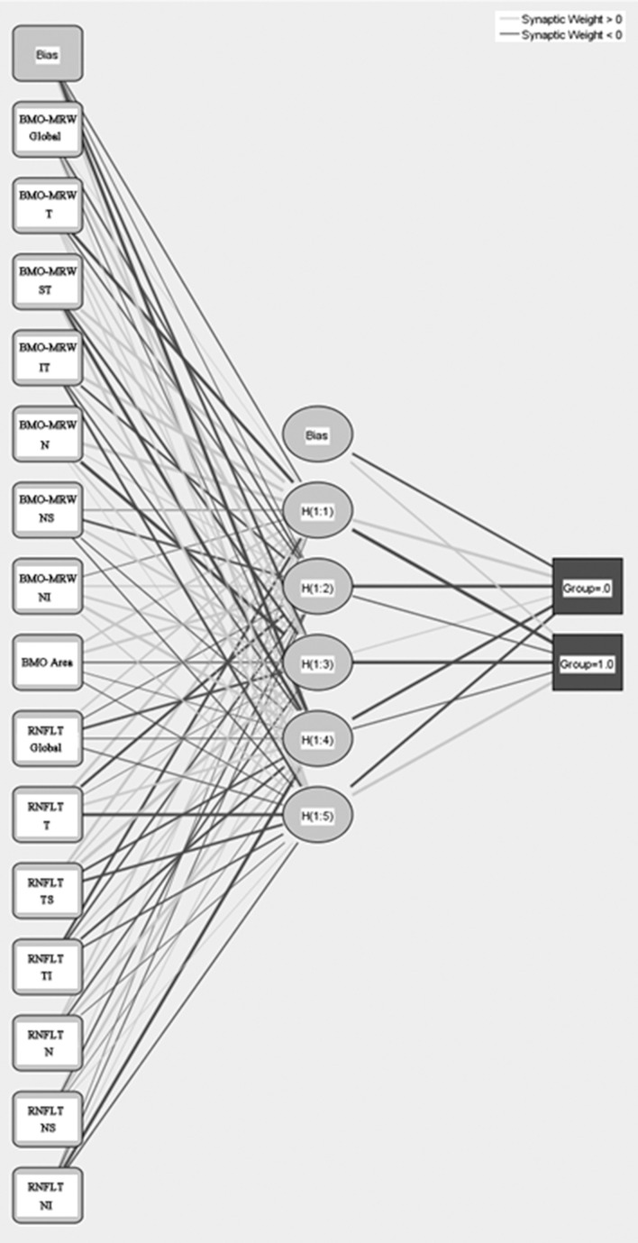
Finally, we used a neural network with one hidden layer consisting of five neurons constructed in SPSS for Windows, version 21.0 (SPSS, Chicago, IL). Input nodes fed into a five-node hidden layer activated by hyperbolic tangent functions. The outputs consisted of two nodes with a softmax function for normal (0) and glaucomatous (1) eyes. We evaluated neural networks with different numbers of hidden layer units and found that the five-unit neural network performed best.

Statistical Analyses

The normality of data distribution was checked using the Kolmogorov–Smirnov test. Clinical characteristics were compared using 1-way analysis of variance or the Kruskal–Wallis test for continuous variables, and the χ² test for categorical variables. A scatterplot of pRNFLT versus BMO-MRW revealed a pRNFLT plateau at high BMO-MRW values and a steep decrease at lower BMO-MRW values. To fit this pattern, we used a nonlinear broken-stick statistical model. The tipping point initially was estimated using the Davies' test,³⁷ and then segmental regression analyses were performed using this initial tipping point as the starting value. Segmental regression analyses were iteratively continued (to reduce errors) until the final tipping point and the two slopes of the broken-stick model (with the corresponding 95% confidence intervals) were determined. Linear and quadratic regression models also were used, with the following equations: y = a + bx (linear), y = a + bx + cx² (quadratic). To compare the fitness of the three regression models, we used Akaike's information criterion (AIC) to estimate the quality of each model relative to those of the other models. Of the various candidate models, the best had the lowest AIC. To compare diagnostic performances, we used the areas under the receiver operating characteristic curves (AUROCs). All statistical analyses were performed using SPSS for Windows, version 21.0 (SPSS) and R (available in the public domain at http://www.R-project.org) with the segmented R library.³⁸ P < 0.05 was considered to reflect statistical significance.

Results

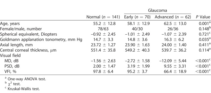
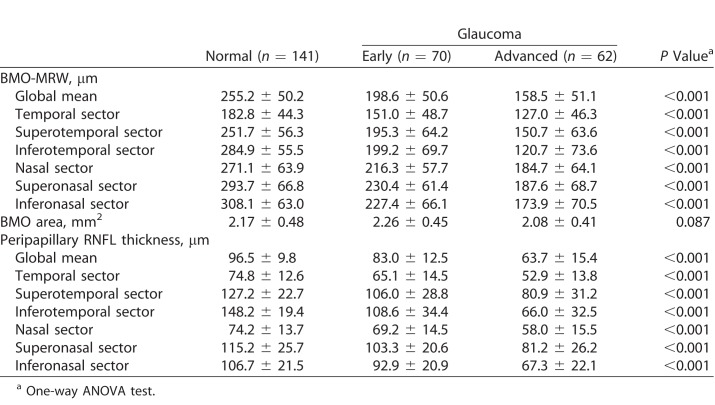
A total of 273 participants were recruited for this study: 141 healthy subjects, and 70 early and 62 advanced glaucoma patients. The demographic data are summarized in Table 1. There were no significant differences in sex, spherical equivalent refractive error, axial length, or central corneal thickness among the groups. Age and IOP became slightly higher as glaucoma progressed. All visual field parameters, such as MD, PSD, and the visual field index (VFI), differed significantly among the three groups. The OCT parameters are summarized in Table 2. Global and all sectoral BMO-MRW and pRNFLT values became significantly thinner as glaucoma progressed, but BMO areas did not differ among the three groups.

Table 1.

Characteristics of the Validation Group

Table 2.

Summary of Average BMO-MRW and Peripapillary RNFL Thicknesses

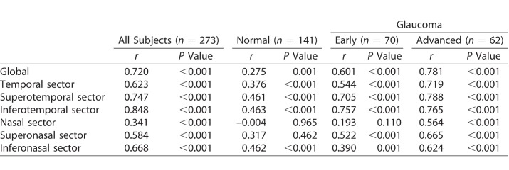
Pearson's correlations between BMO-MRW and pRNFLT values are shown in Table 3. In all subjects group, global and all sectors were significantly correlated. In normal subjects, global and all sectors except for nasal and superonasal sectors were significantly correlated, and correlation coefficients generally were lower than those of the all subjects group. The early glaucoma group exhibited significant correlations globally and for all sectors except the nasal sector; all correlation coefficients were higher than those of the normal group except for the inferonasal sector. In the advanced glaucoma group, significant correlations were evident in global and all sectors, including the nasal sector. The correlation coefficients were higher than those of the early glaucoma group. Together, the results indicated that the correlations between BMO-MRW and pRNFLT became stronger as glaucoma progressed.

Table 3.

Pearson's Correlation Coefficients Between BMO-MRW and Peripapillary RNFL Thickness

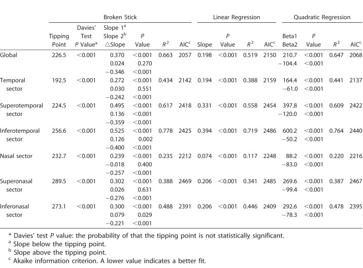
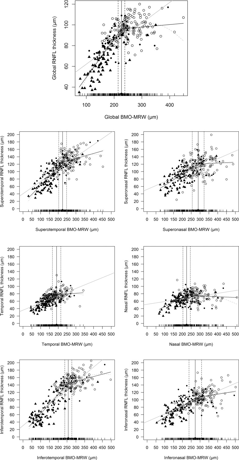
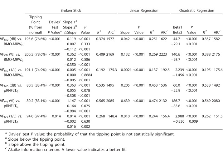
Various regression analyses of BMO-MRW and pRNFLT are summarized in Table 4, and scatterplots are shown in Figure 1. In general, the best-fitting statistical model (with the lowest AIC) was the broken-stick model in the global and most sectors, except for the temporal and superonasal sectors. The worst fitting model was the linear regression model in all sectors. Globally, the tipping point was located at 226.5 μm of BMO-MRW; this was highly significant according to Davies' tests (P < 0.001). The slope above the tipping point was 0.024 (close to zero) and not statistically significant (P = 0.270). However, when the BMO-MRW became thinner than the tipping point, the slope below the tipping point increased sharply to 0.370 and was statistically significant (P < 0.001). These results indicated that the pRNFLT remained almost unchanged until BMO-MRW thinning attained the tipping point, and once BMO-MRW became thinner than the tipping point, pRNFLT began to lose thickness along with BMO-MRW. The temporal sectors generally were better correlated than the nasal sectors (thus, with a larger r² value); the best-correlated sector was the inferotemporal sector (r² = 0.778). Unlike the superonasal and inferonasal sectors (for which the slopes above the tipping point were 0.026 and 0.079, respectively), the superotemporal and inferotemporal sectors, which are the most vulnerable in glaucoma patients, exhibited relatively larger and statistically significant slopes above the tipping point (slope/P value = 0.136/ <0.001 and 0.126/0.002, respectively).

Table 4.

Various Regression Analyses Between BMO-MRW and Peripapillary RNFL Thickness

Figure 1.

Scatterplots between pRNFLT and BMO-MRW values globally (top) and sectorally. Three regression lines are shown: black line, broken-stick model; gray line, linear model; dotted line, quadratic model. Circles represent normal subjects, dots are early glaucoma patients, and triangles are advanced glaucoma patients. Except for the temporal and superonasal sectors, the broken-stick model afforded the best fit.

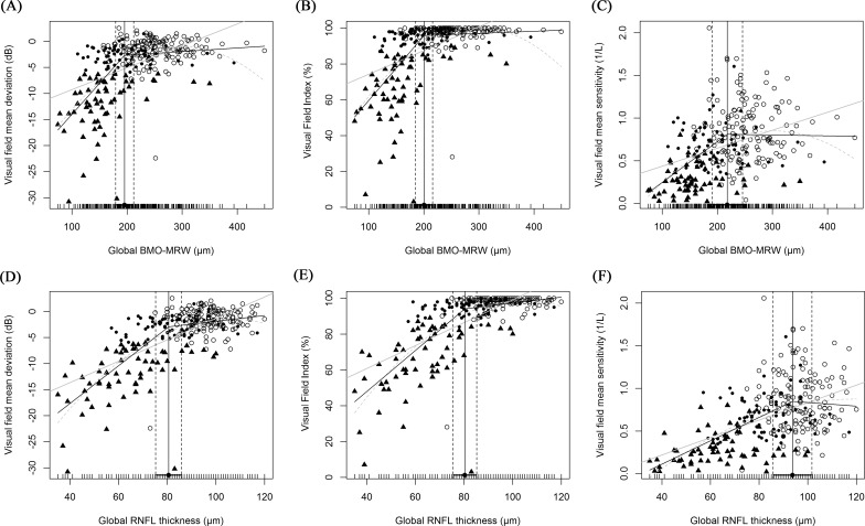
Regression analyses of the BMO-MRW and visual field data are summarized in Table 5, and scatterplots are shown in Figures 2A to 2C. We compared three different measures of the visual field: MD (VF_MD), VFI (VF_VFI), and 1/L, linear, scaled mean sensitivity (VF_MS). The best-fitting regression model for BMO-MRW and visual field data was the broken-stick model, and the worst model was the linear model. The locations of the tipping points were all significant and similar, regardless of the scale of the visual field, being 195.6, 200.5, and 191.1 μm for VF_MD, VF_VFI, and VF_MS, respectively. The slopes above these tipping points were all close to zero: 0.007, 0.012, and 0.000, respectively; no slope was statistically significant. However, the slopes below the tipping points increased sharply to 0.019, 0.362, and 0.005, respectively; all were statistically significant.

Table 5.

Various Regression Analyses Between Visual Field and OCT Parameters

Figure 2.

Scatterplots of visual field and OCT parameters. Three different visual field parameters (MD, VFI, and 1/L) were employed. (A–C) are the scatterplots between visual field data and BMO-MRW. (D–F) are those between visual field data and pRNFLTs. Three regression lines are shown: black line, broken stick model; gray line, linear model; dotted line, quadratic model. Circles represent normal subjects, dots are early glaucoma patients, and triangles are advanced glaucoma patients. The locations of the tipping points between the visual field and BMO-MRW data were similar regardless of the visual field scale used (76.6%, 78.6%, and 74.9% in [A]–[C], respectively). However, when the visual field and pRNFLT data were compared, the tipping points differed by the visual field scale (83.4%, 83.1%, and 97.4% in [D]–[F], respectively).

Regression analyses of pRNFLT and visual field data also are summarized in Table 5, and scatterplots are shown in Figures 2D to 2F. Although the broken-stick model still was significant in this relationship, but different from BMO-MRW, the best-fitting model was the quadratic regression model followed by the broken-stick model, except for VF_MS, which was best fit using the broken-stick model. The differences in the AICs of the broken-stick and quadratic models were almost negligible. The locations of the tipping points were 80.5, 80.2, and 94.0 μm for VF_MD, VF_VFI, and VF_MS, respectively. The tipping point increased significantly when the scale of the visual field was changed from logarithmic (VF_MD and VF_VFI) to linear (VF_MS). It is noteworthy that the tipping point of VF_MS was 94.0 μm, which was approximately 97.4% of the normal pRNFLT in our study cohort. These results indicated that the significant tipping point existed in a linear scale (VF_MS), but most relationships (97.4%) between pRNFLT and VFMS were simply linear.

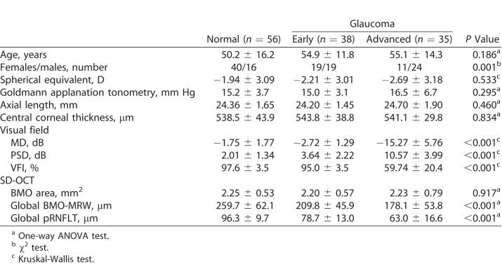
To develop a single combination index using BMO-MRW and pRNFLT, we used a multilayered neural network algorithm. The characteristics of the training dataset for this machine-learning algorithm are summarized in Table 6. We used data from 56 normal subjects, and 38 early and 35 advanced glaucoma patients. There were no significant differences in age, spherical equivalent refractive error, axial length, or central corneal thickness among the groups. All visual field parameters, BMO-MRW, and pRNFLT differed significantly among the groups. We tested many neural networks with different activation functions, input layer parameters, and numbers of hidden layers. Ultimately, we found an optimal network, shown in Figure 3. All sectoral and global BMO-MRWs and pRNFLT parameters, and BMO areas served as the input; and five neurons were contained in a single hidden layer. The activation function was a hyperbolic tangent function, and the output layer was a softmax function (Fig. 3).

Table 6.

Demographic Data Used for Artificial Neural Network Training

Figure 3.

The artificial neural network. BMO-MRW (global and sectoral data), BMO areas, and pRNFLT (global and sectoral data) served as input layers. The activation function is a hyperbolic tangent function and the output layer activation function is a softmax function.

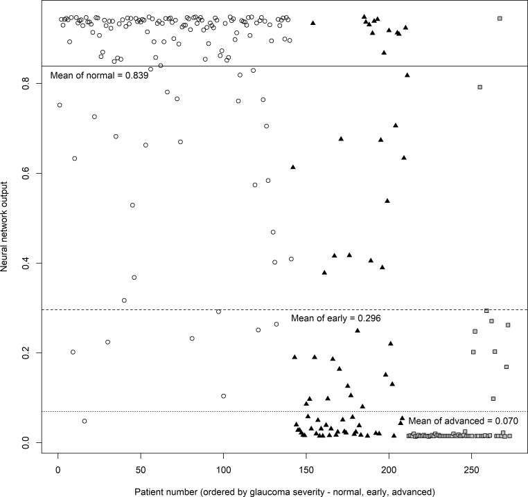
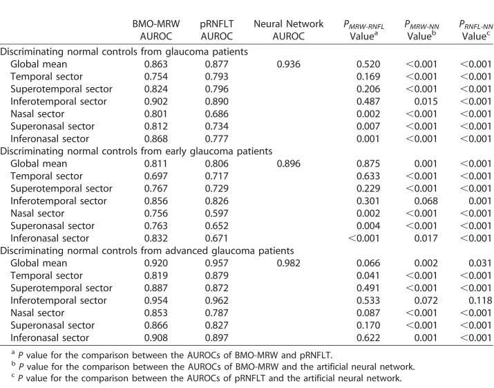
We compared the diagnostic power of BMO-MRW, pRNFLT, and the neural network by measuring AUROCs. The outputs from the neural network are plotted in Figure 4. Average outputs of normal subjects, and those with early and advanced glaucoma, were 0.839, 0.296, and 0.070, respectively. The differences in average outputs between normal and early glaucoma subjects and between early and advanced glaucoma patients were statistically significant (all P < 0.001; Mann–Whitney U test). The AUROCs are summarized in Table 7 and Figure 5. In terms of differentiating normal from glaucoma subjects, BMO-MRW performed significantly better than pRNFLT in all nasal-side sectors (nasal, superonasal, and inferonasal sectors), but not globally or in any temporal-side sector (temporal, superotemporal, and inferotemporal sectors). However, the best diagnostic power was afforded by the neural network, which performed significantly better than the BMO-MRW, with all P < 0.001, except for the inferotemporal sector (P = 0.015). The neural network also performed significantly better than pRNFLT, with all P < 0.001. Overall diagnostic performance fell among all three parameters when differentiating normal from early glaucoma subjects, but the neural network still afforded the best AUROCs. The neural network also was significantly better than the all-sector pRNFLT (P ≤ 0.001) and the all-sector BMO-MRW (P ≤ 0.001), except for the inferotemporal (P = 0.068) and inferonasal (P = 0.017) sectors. However, even in the inferotemporal sector, BMO-MRW (P = 0.068) approached significance. Compared to pRNFLT, BMO-MRW afforded higher AUROCs for most sectors, except the temporal sector. However, statistical significance was attained only for the nasal side sectors (nasal, superonasal, and inferonasal sectors). When differentiating normal from advanced glaucoma subjects, the neural network also exhibited the largest AUROC; however, in the inferotemporal sector, the AUROCs of BMO-MRW and pRNFLT were comparable to that of the neural network (not significantly different). We found no significant differences in BMO-MRW and pRNFLT AUROCs by sector.

Figure 4.

The output values of the artificial neural network for the validation group. Output values close to 1.0 are more likely to be normal than those close to 0, which indicate glaucoma. Circles are normal subjects, triangles are early glaucoma patients, and rectangles are advanced glaucoma patients. The solid horizontal line is the average output value of normal subjects, the dashed horizontal line is that of early glaucoma patients, and the dotted horizontal line is the average output of advanced glaucoma patients. The average output values were 0.839, 0.296, 0.070 (normal, early glaucoma, advanced glaucoma subjects, respectively). The difference in the average output between normal and early glaucoma and early and advanced glaucoma subjects were all statistically significant (all P < 0.001, Mann-Whitney U test).

Table 7.

Comparison of the AUROCs of BMO-MRW, Peripapillary RNFL Thickness, and the Neural Network

Figure 5.

ROC curve of neural network and best parameter of BMO-MRW (inferotemporal sector) and pRNFLT (inferotemporal sector). (A) Normal and glaucoma. AUROC is 0.936, 0.902, 0.890 (neural network, BMO-MRW, pRNFLT respectively). (B) Normal and early glaucoma. AUROC is 0.896, 0.856, 0.826 (neural network, BMO-MRW, pRNFLT respectively). (C) Normal and advanced glaucoma. AUROC is 0.982, 0.954, 0.962 (neural network, BMO-MRW, pRNFLT respectively).

Discussion

The BMO-MRW is a new neuroretinal rim parameter affording better diagnostic accuracy and revealing a more accurate structure–function relationship than the disc margin-based rim area.^17,19,39 In our study, the relationships between BMO-MRW and pRNFLT were not simply linear, being rather closer to a broken-stick model. The BMO-MRW exhibited considerable thinning beforre commencement of pRNFLT thinning. This study is the first to develop a combined index of BMO-MRW and pRNFLT using an artificial neural network model, and to perform correlation analyses. The neural network afforded a significantly better diagnostic performance than either the BMO-MRW or pRNFLT, particularly in terms of discriminating early glaucoma patients.

In terms of the structure–structure relationship between BMO-MRW and pRNFLT, the best-fitting regression model was the broken-stick model, revealing a very significant tipping point. Globally, the slope above the tipping point was almost zero (0.024), but when the BMO-MRW became thinner than the tipping point (226.5 μm; 88.8% of the normal BMO-MRW in our study cohort), the slope increased sharply to 0.370 and BMO-MRW and pRNFLT began to thin simultaneously. Thus, the pRNFLT did not change significantly until BMO-MRW thinning attained the tipping point. In this early phase of glaucoma, the BMO-MRW was most affected. These results are consistent with clinical experience and the findings of previous studies suggesting that many patients may evidence optic disc damage as the first sign of glaucoma progression. An ONH biomechanical study²³ reported that the ONH was the earliest or only site of damage. Stress and strain caused by IOP within the ONH affected not only nutrient delivery but also the supply of blood to retinal ganglion cell (RGC) axons in the presence or absence of laminar deformation. Gardiner et al.²¹ also reported that BMO-MRW was the best parameter for early detection of glaucomatous damage, whereas pRNFLT was the best parameter for monitoring changes. This is because pRNFLT predominantly measures neural tissue (RGC axon bundles) 1.7 mm distant from the optic disc center, whereas BMO-MRW measures the thickness of neuroretinal rim tissue contained within the optic disc. This suggests that BMO-MRW and pRNFLT might complement each other, and if the two parameters were appropriately combined, diagnostic power would be improved for early and advanced glaucoma patients.

The structure–function relationships also differed clearly between BMO-MRW and pRNFLT. The model that best fitted the BMO-MRW data and the visual field parameters was the broken-stick model; very significant tipping points were found at similar locations regardless of the scales of the visual field parameters. The tipping points between BMO-MRW and the visual field data were located at approximately 76.6%, 74.9%, and 76.6% for MD, VFI, and VF_MS, respectively, from the normal BMO-MRW in our study cohort. The slopes above the tipping points were almost zero (0.007, 0.012, and 0.000, respectively), and the visual field did not change until BMO-MRW thinning attained the tipping point. Rapid visual field deterioration commenced after considerable BMO-MRW thinning.

The relationships between pRNFLT and visual field parameters were similar but nonetheless different. A significant tipping point also was found, but the location differed depending on whether a logarithmic (MD and VFI) or linear (VF_MS) scale was used. When using visual field MD and VFI data, the tipping points were located at 83.4% and 83.1%, respectively, from the normal pRNFLT in our study cohort. A very similar finding was reported by Wollstein et al.,⁴⁰ who found that the pRNFLT and visual field MD exhibited a broken-stick relationship, with the tipping point located at approximately 76.7 μm (84.5% of the normal pRNFLT). However, when using the VF_MS, the tipping point increased to 97.4%, which indicates that the relationship between pRNFLT and VF_MS usually is simply linear. The AICs of the broken-stick and linear regression models were similar (148.4 and 156.4, respectively). This suggested that the BMO-MRW and visual field data exhibited a robust broken-stick relationship, whereas the relationships between pRNFLT and visual field data were more affected by the scale. Previous studies support these findings. Schlottmann et al.⁴¹ correlated visual field mean sensitivity on the decibel scale with pRNFLT and found a logarithmic relationship that became linear when decibels were converted into a linear scale. Several investigators have suggested that use of the decibel scale creates artifacts when analyzing structure–function relationships.^35,42 We suggested that the strong broken-stick relationship, regardless of the visual field scale, constitutes further evidence that BMO-MRW is more responsive to early glaucomatous change than is pRNFLT.

We found that the AUROCs of BMO-MRW and pRNFLT generally did not differ significantly. However, for the nasal side sectors (nasal, superonasal, and inferonasal sectors), BMO-MRW yielded significantly higher AUROCs than pRNFLT, because nasal-side pRNFLT was measured using a beam with a high entry angle. The reflectance of the RNFL is highly directional and depends strongly on the angle of illumination,⁴³ probably reducing the reproducibility and diagnostic power of pRNFLT measurements on nasal side sectors. Previous studies have yielded consistent findings. Budenz et al.⁴⁴ reported that nasal pRNFLT quadrant data were the least reproducible of four quadrants. Blumenthal et al.⁴⁵ also reported that such data were the least reproducible, and temporal quadrant data were the most reproducible. However, BMO-MRW data were presumably more reliable in the nasal quadrant because the beam angle at the ONH was not as high as that at the RNFL. We also found that, in terms of discriminating normal from early glaucoma subjects, the global and temporal side (temporal, superotemporal, and inferotemporal sectors) AUROCs of BMO-MRW tended to be higher than those of pRNFLT, although the opposite was observed when discriminating normal from advanced glaucoma subjects. Although the AUROC difference was not statistically significant, given the structure–structure relationships in our study, we assumed that this is because BMO-MRW is more susceptible to early glaucomatous change.

We used a neural network to combine BMO-MRW and pRNFLT data; this was not the first attempt to combine these two parameters. Gmeiner et al.⁴⁶ reported a combined BMO-MRW and peripapillary pRNFLT. They created combined parameters by mathematically adding BMO-MRW to pRNFLT as follows:

To ensure that BMO-MRW and pRNFLT contributed equally to the combined parameter, pRNFLT was multiplied by a factor based on the ratio of mean BMO-MRW to pRNFLT in healthy controls. The largest AUROC among those of BMO-MRW, pRNFLT, and the combined parameter was that of the combined parameter, but the improvement was minor (not statistically significant). Medeiros et al.⁴⁷ also reported improved performance when pRNFLT and ONH data were combined. The largest pRNFLT AUROC was 0.91 in the inferior sector, and the ONH parameter with the largest AUROC was a cup-to-disc ratio of 0.88. Their combined parameter exhibited a significantly improved AUROC of 0.97, but this was not significantly better than the AUROC of pRNFLT (0.91). However, our artificial neural network improved the AUROC very significantly compared to those of the sectoral BMO-MRWs and pRNFLTs. It is important to note that the improvement was not confined to discriminating normal from glaucoma subjects generally, but also normal from early glaucoma subjects. Only the inferotemporal BMO-MRW exhibited an AUROC (0.856) comparable to that of the neural network (0.896), but the AUROC of the neural network was higher and the difference approached significance (P = 0.068).

The neural network has shown a superior ability to combine multiple parameters compared to mathematic combinations of the same parameters. Bowd et al.²⁷ reported the diagnostic performance of a neural network combining 83 optic disc parameters derived via Heidelberg retinal tomography. This combined index better discriminated glaucomatous from healthy eyes than did an earlier linear discriminant function (LDF). It was suggested that neural networks were at least as useful as LDFs. Goldbaum et al.⁴⁸ compared three machine-learning algorithms, including a neural network, in terms of standard automated perimetry interpretation. The neural network performed better than mathematic index combinations involving the visual field MD, PSD, and LDF. A neural network can classify complex variables even if the inputs are heterogeneous. Brigatti et al.²⁸ reported an improved diagnostic performance of a neural network combining visual field parameters (mean deviation, corrected loss variance, and short-term fluctuations) and structural data (cup-to-disc ratio, rim area, cup volume, and pRNFLT) derived via OCT. The neural network better discriminated between normal and early glaucoma subjects than analyses using only structural data. Our neural network effectively and complementarily combined the heterogeneous parameters BMO-MRW and pRNFLT to significantly improve diagnostic power. The BMO areas did not significantly differ among our groups. However, Gmeiner et al.⁴⁶ reported that the BMO area influenced the diagnostic power of BMO-MRW and pRNFLT; a larger BMO area significantly decreased the AUROCs of BMO-MRW and pRNFLT. Consistent with these results, addition of the BMO area to the neural network improved performance.

A strength of our study is that we used data from a relatively large number of patients: 402 divided into validation (273) and neural net training (129) groups. When preparing the training set, we were particularly careful to match age and number between normal and glaucoma subjects when selecting those whose OCT data exhibited good signal-to-noise ratios. Overfitting is a major problem when developing a neural network and is even more severe during deep learning; neural networks can have large numbers of layers containing many neurons, up to millions. Performance variability is reduced by increasing the size of the training set.⁴⁹ There is no absolute rule indicating how much training data are required. However, in previous studies, relatively smaller training sets afforded better performance. Brigatti et al.⁵⁰ used data from 233 patients to develop and validate automated detection of a glaucomatous visual field. Goldbaum et al.⁵¹ used data from 120 patients in a similar study. Uchida et al.⁵² used data from 96 patients when exploring whether confocal laser images revealed glaucomatous structural damage. Another strength of our study is that BMO-MRW and pRNFLT exhibited a complementary relationship and could be measured simultaneously. By combining these complementary parameters, clinicians should be able to improve diagnoses without the need to perform two different examinations.

Our study had certain limitations. We found a broken-stick relationship between BMO-MRW and pRNFLT. However, in the normal group, the correlation coefficient was lower than in the glaucoma group. Thus, it is possible that the broken-stick relationship could reflect different correlations in the normal and glaucoma groups; further longitudinal studies are necessary. Another limitation was that, although we believed that our single combined index might aid clinicians, further studies comparing the performance of clinicians using the combined index to that of clinicians using only individual parameters are required.

In conclusion, the neural network significantly improved diagnostic power by combining BMO-MRW and pRNFLT data. This single unified index performed better than either BMO-MRW or pRNFLT data alone, and should help clinicians make faster and more reliable decisions, particularly when the predictions of multiple parameters disagree. We believed that our neural network might find applications in ophthalmic research. The diagnostic power can be improved by simply adding new parameters to the input layer. We also found that the relationship between BMO-MRW and pRNFLT was well-represented by the broken-stick model. Before the pRNFLT began to thin, considerable BMO-MRW thinning was evident, which suggested that the BMO-MRW is more sensitive than RNFL to early glaucomatous changes.

References

- 1.Resnikoff S, Pascolini D, Etya'ale D, et al. Global data on visual impairment in the year 2002. Bull World Health Organ. 2004;82:844–851. [PMC free article] [PubMed] [Google Scholar]
- 2.Tham Y-, Li X, Wong T, Quigley H, Aung T, Cheng C-Y. Global prevalence of glaucoma and projections of glaucoma burden through 2040: a systematic review and meta-analysis. Ophthalmology. 2014;121:2081–2090. doi: 10.1016/j.ophtha.2014.05.013. [DOI] [PubMed] [Google Scholar]
- 3.Sommer A, Pollack I, Maumenee AE. Optic disc parameters and onset of glaucomatous field loss: I. Methods and progressive changes in disc morphology. Arch Ophthalmol. 1979;97:1444–1448. doi: 10.1001/archopht.1979.01020020106002. [DOI] [PubMed] [Google Scholar]
- 4.Read R, Spaeth GL. The practical clinical appraisal of the optic disc in glaucoma: the natural history of cup progression and some specific disc-field correlations. Trans-Am Acad Ophthalmol Otolaryngol Am Acad Ophthalmol Otolaryngol. 1974;78:OP255. [PubMed] [Google Scholar]
- 5.Kamal D, Viswanathan A, Garway-Heath D, Hitchings R, Poinoosawmy D, Bunce C. Detection of optic disc change with the Heidelberg retina tomograph before confirmed visual field change in ocular hypertensives converting to early glaucoma. Br J Ophthalmol. 1999;83:290–294. doi: 10.1136/bjo.83.3.290. [DOI] [PMC free article] [PubMed] [Google Scholar]
- 6.Quigley H, Addicks E, Green WR. Optic nerve damage in human glaucoma: III. Quantitative correlation of nerve fiber loss and visual field defect in glaucoma, ischemic neuropathy, papilledema, and toxic neuropathy. Arch Ophthalmol. 1982;100:135–146. doi: 10.1001/archopht.1982.01030030137016. [DOI] [PubMed] [Google Scholar]
- 7.Ugurlu S, Hoffman D, Garway-Heath D, Caprioli J. Relationship between structural abnormalities and short-wavelength perimetric defects in eyes at risk of glaucoma. Am J Ophthalmol. 2000;129:592–598. doi: 10.1016/s0002-9394(99)00445-6. [DOI] [PubMed] [Google Scholar]
- 8.Sommer A, Katz J, Quigley H, et al. Clinically detectable nerve fiber atrophy precedes the onset of glaucomatous field loss. Arch Ophthalmol. 1991;109:77–83. doi: 10.1001/archopht.1991.01080010079037. [DOI] [PubMed] [Google Scholar]
- 9.Group EGPS (EGPS), others. Results of the European Glaucoma Prevention Study. Ophthalmology. 2005;112:366–375. doi: 10.1016/j.ophtha.2004.11.030. [DOI] [PubMed] [Google Scholar]
- 10.Quigley H, Katz J, Derick R, Gilbert D, Sommer A. An evaluation of optic disc and nerve fiber layer examinations in monitoring progression of early glaucoma damage. Ophthalmology. 1992;99:19–28. doi: 10.1016/s0161-6420(92)32018-4. [DOI] [PubMed] [Google Scholar]
- 11.Kass M, Heuer D, Higginbotham E, et al. The Ocular Hypertension Treatment Study: a randomized trial determines that topical ocular hypotensive medication delays or prevents the onset of primary open-angle glaucoma. Arch Ophthalmol. 2002;120:701–713. doi: 10.1001/archopht.120.6.701. [DOI] [PubMed] [Google Scholar]
- 12.Belghith A, Medeiros F, Bowd C, et al. Structural change can be detected in advanced-glaucoma eyes. Invest Ophthalmol Vis Sci. 2016;57:OCT511–518. doi: 10.1167/iovs.15-18929. [DOI] [PMC free article] [PubMed] [Google Scholar]
- 13.Sung K, Sun J, Na J, Lee J, Lee Y. Progression detection capability of macular thickness in advanced glaucomatous eyes. Ophthalmology. 2012;119:308–313. doi: 10.1016/j.ophtha.2011.08.022. [DOI] [PubMed] [Google Scholar]
- 14.Shin J, Sung K, Lee G, Durbin M, Cheng D. Ganglion cell-inner plexiform layer change detected by optical coherence tomography indicates progression in advanced glaucoma. Ophthalmology. 2017;124:1466–1474. doi: 10.1016/j.ophtha.2017.04.023. [DOI] [PubMed] [Google Scholar]
- 15.Greaney M, Hoffman D, Garway-Heath D, Nakla M, Coleman A, Caprioli J. Comparison of optic nerve imaging methods to distinguish normal eyes from those with glaucoma. Invest Ophthalmol Vis Sci. 2002;43:140–145. [PubMed] [Google Scholar]
- 16.Xu G, Weinreb R, Leung CKS. Optic nerve head deformation in glaucoma: the temporal relationship between optic nerve head surface depression and retinal nerve fiber layer thinning. Ophthalmology. 2014;121:2362–2370. doi: 10.1016/j.ophtha.2014.06.035. [DOI] [PubMed] [Google Scholar]
- 17.Chauhan B, O'Leary N, AlMobarak F, et al. Enhanced detection of open-angle glaucoma with an anatomically accurate optical coherence tomography–derived neuroretinal rim parameter. Ophthalmology. 2013;120:535–543. doi: 10.1016/j.ophtha.2012.09.055. [DOI] [PMC free article] [PubMed] [Google Scholar]
- 18.Danthurebandara V, Sharpe G, Hutchison D, et al. Enhanced structure–function relationship in glaucoma with an anatomically and geometrically accurate neuroretinal rim measurement: Structure–function relationship in glaucoma. Invest Ophthalmol Vis Sci. 2015;56:98–105. doi: 10.1167/iovs.14-15375. [DOI] [PubMed] [Google Scholar]
- 19.Pollet-Villard F, Chiquet C, Romanet J-, Noel C, Aptel F. Structure–function relationships with spectral-domain optical coherence tomography retinal nerve fiber layer and optic nerve head measurements. Invest Ophthalmol Vis Sci. 2014;55:2953. doi: 10.1167/iovs.13-13482. [DOI] [PubMed] [Google Scholar]
- 20.So Hee Kim MD. Diagnostic accuracies of Bruch membrane opening-minimum rim width and retinal nerve fiber layer thickness in glaucoma. J Korean Ophthalmol Soc. 2017;58:836–845. [Google Scholar]
- 21.Gardiner S, Boey P, Yang H, Fortune B, Burgoyne C, Demirel S. Structural measurements for monitoring change in glaucoma: comparing retinal nerve fiber layer thickness with minimum rim width and area: Structural measurements of change in glaucoma. Invest Ophthalmol Vis Sci. 2015;56:6886–6891. doi: 10.1167/iovs.15-16701. [DOI] [PMC free article] [PubMed] [Google Scholar]
- 22.Fortune B, Reynaud J, Hardin C, Wang L, Sigal I, Burgoyne CF. Experimental glaucoma causes optic nerve head neural rim tissue compression: a potentially important mechanism of axon injury. Invest Ophthalmol Vis Sci. 2016;57:4403–4411. doi: 10.1167/iovs.16-20000. [DOI] [PMC free article] [PubMed] [Google Scholar]
- 23.Burgoyne CF. A biomechanical paradigm for axonal insult within the optic nerve head in aging and glaucoma. Exp Eye Res. 2011;93:120–132. doi: 10.1016/j.exer.2010.09.005. [DOI] [PMC free article] [PubMed] [Google Scholar]
- 24.Leung C, Chan W, Hui Y, et al. Analysis of retinal nerve fiber layer and optic nerve head in glaucoma with different reference plane offsets, using optical coherence tomography. Invest Ophthalmol Vis Sci. 2005;46:891–899. doi: 10.1167/iovs.04-1107. [DOI] [PubMed] [Google Scholar]
- 25.Downs J, Yang H, Girkin C, et al. Three-dimensional histomorphometry of the normal and early glaucomatous monkey optic nerve head: neural canal and subarachnoid space architecture. Invest Ophthalmol Vis Sci. 2007;48:3195–3208. doi: 10.1167/iovs.07-0021. [DOI] [PMC free article] [PubMed] [Google Scholar]
- 26.Yang H, Downs J, Girkin C, et al. 3-D histomorphometry of the normal and early glaucomatous monkey optic nerve head: Lamina cribrosa and peripapillary scleral position and thickness. Invest Ophthalmol Vis Sci. 2007;48:4597–4607. doi: 10.1167/iovs.07-0349. [DOI] [PMC free article] [PubMed] [Google Scholar]
- 27.Bowd C, Chan K, Zangwill L, et al. Comparing neural networks and linear discriminant functions for glaucoma detection using confocal scanning laser ophthalmoscopy of the optic disc. Invest Ophthalmol Vis Sci. 2002;43:3444–3454. [PubMed] [Google Scholar]
- 28.Brigatti L, Hoffman D, Caprioli J. Neural networks to identify glaucoma with structural and functional measurements. Am J Ophthalmol. 1996;121:511–521. doi: 10.1016/s0002-9394(14)75425-x. [DOI] [PubMed] [Google Scholar]
- 29.Mazurowski M, Habas P, Zurada J, Lo J, Baker J, Tourassi GD. Training neural network classifiers for medical decision making: the effects of imbalanced datasets on classification performance. Neural Netw. 2008;21:427–436. doi: 10.1016/j.neunet.2007.12.031. [DOI] [PMC free article] [PubMed] [Google Scholar]
- 30.Foster P, Buhrmann R, Quigley H, Johnson GJ. The definition and classification of glaucoma in prevalence surveys. Br J Ophthalmol. 2002;86:238–242. doi: 10.1136/bjo.86.2.238. [DOI] [PMC free article] [PubMed] [Google Scholar]
- 31.Cello K, Nelson-Quigg J, Johnson CA. Frequency doubling technology perimetry for detection of glaucomatous visual field loss. Am J Ophthalmol. 2000;129:314–322. doi: 10.1016/s0002-9394(99)00414-6. [DOI] [PubMed] [Google Scholar]
- 32.Wu H, de Boer J, Chen TC. Reproducibility of retinal nerve fiber layer thickness measurements using spectral domain optical coherence tomography. J Glaucoma. 2011;20:470–476. doi: 10.1097/IJG.0b013e3181f3eb64. [DOI] [PMC free article] [PubMed] [Google Scholar]
- 33.Alasil T, Wang K, Yu F, et al. Correlation of retinal nerve fiber layer thickness and visual fields in glaucoma: a broken stick model. Am J Ophthalmol. 2014;157:953–959. doi: 10.1016/j.ajo.2014.01.014. [DOI] [PMC free article] [PubMed] [Google Scholar]
- 34.Garway-Heath D, Poinoosawmy D, Fitzke F, Hitchings RA. Mapping the visual field to the optic disc in normal tension glaucoma eyes. Ophthalmology. 2000;107:1809–1815. doi: 10.1016/s0161-6420(00)00284-0. [DOI] [PubMed] [Google Scholar]
- 35.Hood D, Kardon RH. A framework for comparing structural and functional measures of glaucomatous damage. Prog Retin Eye Res. 2007;26:688–710. doi: 10.1016/j.preteyeres.2007.08.001. [DOI] [PMC free article] [PubMed] [Google Scholar]
- 36.Amato F, López A, Peña-Méndez E, Vaňhara P, Hampl A, Havel J. Artificial Neural Networks in Medical Diagnosis. New York: Elsevier;; 2013. [Google Scholar]
- 37.Davies RB. Hypothesis testing when a nuisance parameter is present only under the alternative. Biometrika. 1987;74:33–43. [Google Scholar]
- 38.Muggio VMR. Segmented: an R package to fit regression models with broken-line relationships. R News. 2008;8:20–25. [Google Scholar]
- 39.Malik R, Belliveau A, Sharpe G, Shuba L, Chauhan B, Nicolela MT. Diagnostic accuracy of optical coherence tomography and scanning laser tomography for identifying glaucoma in myopic eyes. Ophthalmology. 2016;123:1181–1189. doi: 10.1016/j.ophtha.2016.01.052. [DOI] [PubMed] [Google Scholar]
- 40.Wollstein G, Kagemann L, Bilonick R, et al. Retinal nerve fibre layer and visual function loss in glaucoma: the tipping point. Br J Ophthalmol. 2012;96:47–52. doi: 10.1136/bjo.2010.196907. [DOI] [PMC free article] [PubMed] [Google Scholar]
- 41.Schlottmann P, De Cilla S, Greenfield D, Caprioli J, Garway-Heath DF. Relationship between visual field sensitivity and retinal nerve fiber layer thickness as measured by using scanning laser polarimetry. Invest Ophthalmol Vis Sci. 2004;45:1823. doi: 10.1167/iovs.03-0692. [DOI] [PubMed] [Google Scholar]
- 42.Harwerth R, Carter-Dawson L, Smith E, Barnes G, Holt W, Crawford ML. Neural losses correlated with visual losses in clinical perimetry. Invest Ophthalmol Vis Sci. 2004;45:3152–3160. doi: 10.1167/iovs.04-0227. [DOI] [PubMed] [Google Scholar]
- 43.Tun T, Sun C-, Baskaran M, et al. Determinants of optical coherence tomography–derived minimum neuroretinal rim width in a normal Chinese population: OCT-derived BMO-MRW in a normal Chinese population. Invest Ophthalmol Vis Sci. 2015;56:3337–3344. doi: 10.1167/iovs.15-16786. [DOI] [PubMed] [Google Scholar]
- 44.Budenz D, Fredette M-, Feuer W, Anderson DR. Reproducibility of peripapillary retinal nerve fiber thickness measurements with stratus OCT in glaucomatous eyes. Ophthalmology. 2008;115:661–666. doi: 10.1016/j.ophtha.2007.05.035. [DOI] [PubMed] [Google Scholar]
- 45.Blumenthal E, Williams J, Weinreb R, Girkin C, Berry C, Zangwill LM. Reproducibility of nerve fiber layer thickness measurements by use of optical coherence tomography. Ophthalmology. 2000;107:2278–2282. doi: 10.1016/s0161-6420(00)00341-9. [DOI] [PubMed] [Google Scholar]
- 46.Gmeiner J, Schrems W, Mardin C, Laemmer R, Kruse F, Schrems-Hoesl LM. Comparison of Bruch's membrane opening minimum rim width and peripapillary retinal nerve fiber layer thickness in early glaucoma assessment: BMO-MRW and RNFLT in early glaucoma assessment. Invest Ophthalmol Vis Sci. 2016;57:OCT575–OCT584. doi: 10.1167/iovs.15-18906. [DOI] [PubMed] [Google Scholar]
- 47.Medeiros F, Zangwill L, Bowd C, Vessani R, Susanna R, Weinreb RN. Evaluation of retinal nerve fiber layer, optic nerve head, and macular thickness measurements for glaucoma detection using optical coherence tomography. Am J Ophthalmol. 2005;139:44–55. doi: 10.1016/j.ajo.2004.08.069. [DOI] [PubMed] [Google Scholar]
- 48.Goldbaum M, Sample P, Chan K, et al. Comparing machine learning classifiers for diagnosing glaucoma from standard automated perimetry. Invest Ophthalmol Vis Sci. 2002;43:162–169. [PubMed] [Google Scholar]
- 49.Lawrence S, Giles CL. Neural Networks2000. IJCNN 2000Proceedings of the IEEE-INNS-ENNS International Joint Conference On Neural Networks Vol 1. IEEE; 2000. Overfitting and neural networks: conjugate gradient and backpropagation; pp. 114–119. Available at: http://ieeexplore.ieee.org/abstract/document/857823/ [Google Scholar]
- 50.Brigatti L, Nouri-Mahdavi K, Weitzman M, Caprioli J. Automatic detection of glaucomatous visual field progression with neural networks. Arch Ophthalmol. 1997;115:725–728. doi: 10.1001/archopht.1997.01100150727005. [DOI] [PubMed] [Google Scholar]
- 51.Goldbaum M, Sample P, White H, et al. Interpretation of automated perimetry for glaucoma by neural network. Invest Ophthalmol Vis Sci. 1994;35:3362–3373. [PubMed] [Google Scholar]
- 52.Uchida H, Brigatti L, Caprioli J. Detection of structural damage from glaucoma with confocal laser image analysis. Invest Ophthalmol Vis Sci. 1996;37:2393–2401. [PubMed] [Google Scholar]